Monocular Depth Estimation Algorithm Integrating Parallel Transformer and Multi-Scale Features

Abstract

In the process of environmental perception, traditional CNN is often unable to effectively capture global context information due to its network structure, which leads to the problem of blurred edges of objects and scenes. Aiming at this problem, a self-supervised monocular depth estimation algorithm incorporating a Transformer is proposed. First of all, the encoder-decoder architecture is adopted. In the course of the encoding procedure, the input image generates images with different patch sizes but the same size. The multi-path Transformer network and single-path CNN network are used to extract global and local features, respectively, and feature fusion is achieved through interactive modules, which improves the network’s ability to acquire global information. Second, a multi-scale fusion structure of hierarchical features is designed to improve the utilization of features of different scales. Experiments for training the model were conducted using the KITTI dataset. The outcomes reveal that the proposed algorithm outperforms the mainstream algorithm. Compared with the latest CNN-Transformer algorithm, the proposed algorithm reduces the absolute relative error by 3.7% and the squared relative error by 3.9%.

1. Introduction

With the rapid development of artificial intelligence, unmanned driving, intelligent robots, augmented reality (AR), and other technologies have received more attention, and the core of such technologies is environmental perception. Depth estimation is a key part of environmental perception. Accurate and rapid estimation of the distance between the ontology and the target is the basis for cognition and control [1]. Traditional depth estimation methods include using lidar or multi-eye cameras to obtain scale information, and calculating scale based on camera motion and pose information. The more classic algorithms include recovery from motion (Structure from Motion, SFM), using monocular the image sequence captured by the camera estimates depth [2], multiview reconstruction (Multiview System, MVS) [3,4], triangulation (Triangulation) [5,6], etc. These methods are based on continuous image information and known camera pose information. They have high requirements for the collection of initial information and are difficult to estimate the depth of an individual image. There are also many methods that rely on multi-image features, such as: recovering from shadows (Shape from Shading) [7], obtaining scale from focus or defocus (Depth from Focus or Depth from Defocus) [8,9], etc. Most of the features collected by these methods are not rich enough, which seriously affects the accuracy of depth estimation.

After the advent of deep learning, a wealth of feature information can be extracted from images through convolutional neural networks, which overcomes the above deficiencies, enabling monocular depth estimation to quickly complete image recognition, so it has been greatly developed. Monocular depth estimation using deep learning is divided into supervised learning and self-supervised learning. Supervised learning uses image information with calibrated depth parameters for model training, but the cost of obtaining a multitude of pictures with real surface depth is too high, and the labels are sparse, which is not suitable for ground estimation. Self-supervised learning algorithms do not require labeled data for training, greatly reducing training costs. Garg et al. [10] first proposed a self-supervised training framework, which consists of two parts: deep network and image reconstruction. It uses image pairs for depth estimation, reconstructs a new view, and then compares it with the original view to complete the training. Zhou et al. [11] proposed a method of video training, designing a depth estimation network and pose estimation network, using each frame of the video as a training set to train the network, and using the image reconstruction minimum loss function to make the network convergence. Godard et al. [12] proposed the minimum reprojection error formula, which improves the robustness of the algorithm in environments where objects are occluded and reduce boundary artifacts by using multiple scale appearance matching losses. Such depth estimation methods are all based on CNN for research. However, due to the convolution operation principle of CNN, its receptive field is limited, which shows shortcomings in the acquisition of global remote information, reducing the effectiveness of self-supervised learning. To solve this problem, most of the algorithm models developed based on CNN will build a deeper backbone or complex architecture, which leads to a larger model size and increases the computational workload.

In addressing the aforementioned issues, this paper suggests an approach to use the Transformer network to improve the existing CNN network algorithm. Improved on the basis of U-net network architecture, the backbone network was modified into a multi-path Transformer and CNN fusion network, using the global feature to local feature interaction module (GLI) for feature fusion, combining the feature information extracted by the two networks. The combination enriches the effectiveness of image feature expression, thereby solving the problem of object and scene edge blur caused by insufficient global features of CNN in self-supervised learning. The contributions of this paper can be summarized in two aspects.

(1)

A new algorithm incorporating a new backbone network is proposed for self-supervised monocular depth estimation. This method solves the problem of limited receptive fields in a separate CNN network by using a parallel Transformer network and makes a certain contribution to increasing feature richness and effectiveness.

(2)

Compared with existing similar algorithms, the proposed new algorithm shows higher accuracy on the KITTI dataset and achieves better results under the same conditions through improvements. The effectiveness of the improvements in each part of this article is demonstrated through ablation experiments.

2. Related Work

This section will further introduce research related to monocular depth estimation and the application of transformers in monocular depth estimation.

2.1. Deep Learning and Monocular Depth Estimation

Depth estimation is an uncertain task. The same two-dimensional image scene may correspond to multiple three-dimensional scenes. Deep learning methods are divided into two types: supervised and self-supervised.

Supervised depth estimation extracts features from images through a deep network, uses images with real depth as supervision signals, and learns the relationship between image information and depth. Eigen et al. [13] were the first to use deep learning methods to complete the depth estimation task from a single image. They use multi-scale networks to extract image features with different levels of finesse. Laina et al. [14] used pre-trained encoders with new upsampling modules and loss functions to improve the training effect. Ramamonjisoa et al. [15] proposed to predict the residual depth map by refining the network, which improved the accuracy of the first estimation result.

Self-supervised depth estimation does not need to rely on real-depth images as supervision signals and is trained using image pairs or videos without ground truth. Garg et al. [10] and Zhou et al. [11] proposed training methods through image pairs and videos, respectively. They all regarded depth estimation as an image reconstruction task and allowed the network to converge through the loss during reconstruction. Godard et al. [16] first proposed the left and right disparity consistent loss to improve the estimation accuracy, and then further proposed the minimum photometric loss in [12] to reduce the impact of occlusion and improve the robustness. In subsequent research, some people have introduced more constraints for dynamic scenes, such as the optical flow method [17], semantic segmentation [18], etc.

2.2. Application of Transformer in Monocular Depth Estimation

Research related to monocular depth estimation is mostly based on CNN, such as using the algorithm using ResNet18 [19] as the backbone network. With the emergence of transformer networks and breakthroughs in various fields of computer vision, some research on depth estimation based on transformers has also emerged. Varma et al. [20] used the Transformer network for self-supervised monocular depth estimation. Bae et al. [21] proposed a network that integrates CNN and transformer, which enhanced the feature richness of CNN at a certain level. Zhang [22] et al. proposed a lightweight CNN-Transformer network, which reduced the amount of calculation while retaining a certain accuracy by designing a new architecture.

3. Self-Supervised Learning Network Structure

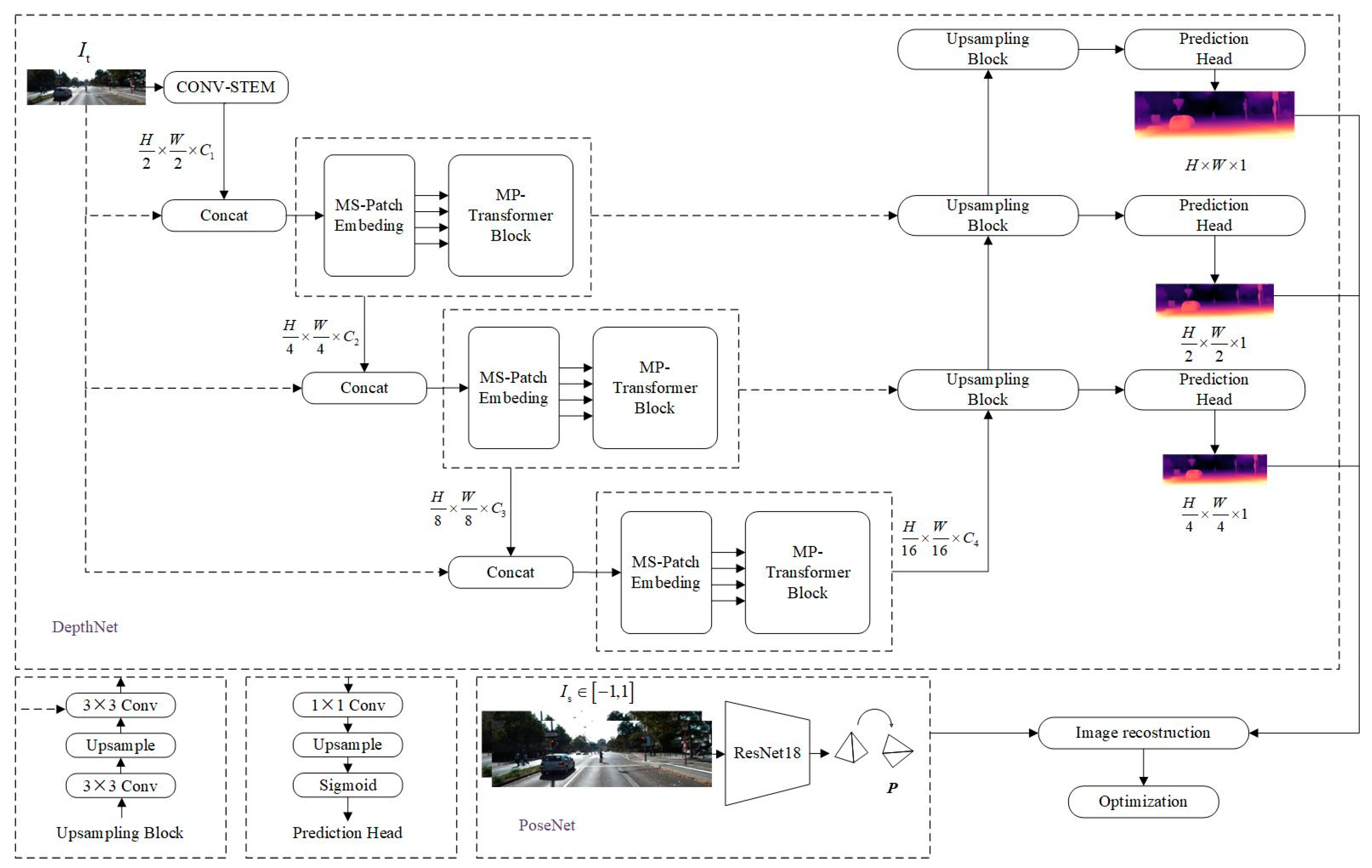
The network structure proposed in this article uses a similar architecture to Monodepth2 [12], including depth and pose networks, which play the role of image depth estimation and camera pose estimation, respectively. The depth estimation network uses the U-net network architecture modified by the fusion Transformer network to encode and decode, and the input is an individual RGB image; the pose estimation network leverages the ResNet18 architecture to infer the camera’s pose by analyzing a continuous stream of image data, and the input consists of a set of two RGB images. A new network structure is formed by using a parallel Transformer network and multi-scale feature fusion, as depicted in Figure 1.

3.1. DepthNet

Differing from supervised depth estimation approaches, self-supervised estimation methods obtain their supervision signal through image reprojection from diverse viewpoints. For achieving satisfactory results, it is necessary to accurately distinguish the scene structure for depth estimation. It is not easy to distinguish between foreground objects and background objects. The current algorithm based on traditional CNN uses convolutional layers to aggregate full-text contextual information and improves model performance through hierarchical union and atrous convolution. However, complex network structures also make it difficult to improve algorithm accuracy. At the same time, owing to the constraints of conventional convolution, it becomes arduous to model the global appearance similarity of objects, and there will be situations where foreground objects and background objects cannot be clearly distinguished in shallow networks.

The Transformer network has a self-attention mechanism (Self-attention), which has excellent performance in the recognition of global context information and has made progress in computer vision research domains like image classification and target detection. In the domain of monocular depth estimation, relying on the Transformer network can break through the limitations of the traditional convolutional network and better extract feature information. This paper uses MPVIT [23], one of the latest Transformer architectures, to optimize the algorithm by modifying the architecture of the backbone network, and uses parallel multi-path modules to extract local and global features.

The overall depth estimation network proposed in this article uses U-net’s encoding-decoding structure, which can be divided into four stages, and features of different scales are gathered in each stage. Input an image of size $H\times W\times 3$, send the image to the convolution system, first perform downsampling through a 3 × 3 convolution, and then perform feature extraction and scale adjustment through two 3 × 3 convolutions using a stride of 1, outputting a feature map of size $H/2\times W/2\times C_1$. After entering the second stage, the feature map is spliced with the pooled original input image. This splicing method can help alleviate the loss of spatial information details from size reduction. Here, the same processing method as Lite-Mono [22] is used. The third stage and the fourth stage also do similar processing. The multi-scale patch embedding module and the multi-path Transformer module are used in the second to fourth stages, as shown in Figure 1.

The multi-scale patch embedding module can change the sequence length of the resulting image patches by adjusting the stride and padding length, and then output features with different patch sizes but the same size. By embedding patches of different scales, we can simultaneously utilize fine-grained and coarse-grained visual information at the identical feature level, allowing us to more comprehensively capture the information in the image and improve the expressiveness and accuracy of the model. As can be seen in Figure 2 above, the initial image undergoes preprocessing to generate three patches with sizes of 3 × 3, 5 × 5, and 7 × 7, and then features of the same size are generated by adjusting the transformation stride and padding length. This process is carried out through a sequence of three successive 3 × 3 convolutional layers. The channel size is $C$, the padding is 1, and the stride is set according to whether the resolution needs to be adjusted. It is 2 when needed and 1 when not. For the feature $X_2\in R^{H_2\times W_2\times C_2}$ of the second stage, features $F_{3\times 3}\left(X_2\right)$, $F_{5\times 5}\left(X_2\right)$, and $F_{7\times 7}\left(X_2\right)$ with size $H/4\times W/4\times C_2$ can be generated. In this paper, four parallel convolutions are used to generate features with the same size and different receptive field sizes, and these features are sent to the multi-path Transformer module with four branches, as shown in Figure 3.

In the multi-path Transformer module, a deep residual bottleneck block and three parallel Transformer blocks are used to accept and process the transmitted features, and then two types of features are aggregated through the global-to-local feature interaction module (GLI) while using the local connectivity of CNN and the global context of Transformer are used to represent rich features. The single-path deep residual bottleneck block is composed of three convolutional layers: 1 × 1 convolution, 3 × 3 depth convolution, and 1 × 1 convolution, using residual connection, the channel size is $C_{\mathrm{i}}$. This module is used to obtain local features $L^i\in R^{H_{\mathrm{i}}\times W_{\mathrm{i}}\times C_{\mathrm{i}}}$. To reduce the computational burden of the three parallel Transformer blocks, the decomposition self-attention mechanism in CoaT [24] is used here:

$$FactorAtt(Q,K,V)=\frac{Q}{\sqrt{C}}(softmax{(K)}^{T}V),$$

(1)

where $Q,K,V\in R^{N\times C}$ is the query, key, and value obtained by linear projection, and $C$ is the embedding dimension. The attention mechanism used in [24] simplifies the attention by modifying $\varphi (·)$ and $\psi (·)$. The $\varphi (·)$ is set to $1/\sqrt{C}$ and $\psi (·)$ is set to a softmax function, thereby improving the computational efficiency of the attention mechanism. Multi-path transform is used in this article, which undoubtedly increases the amount of calculation and requires some adjustment of parameters to reduce the amount of calculation. Analyzing the complexity of the operation shows that adjusting the channel $C$ can achieve better results than other parameters. Therefore, this article sets different settings for $C$ at different stages to reduce the amount of calculation while ensuring network performance.

The global features $G_{i,j}\in R^{H_i\times W_i\times C_i}$ are represented by the Transformer, and then aggregate two types of features represented, using the concatenation operation:

$$A_i=Concat\left(\left[L_i,G_{i,0},G_{i,1},G_{i,2},\cdots ,,G_{i,j}\right]\right),$$

(2)

$$X_{i+1}=H\left(A_i\right).$$

(3)

where $j$ represents the path number of the Transformer block, $A_i\in R^{H_i\times W_i\times \left(1+j\right)C_i}$ is the feature generated after concatenation, $H(·)$ represents a function that learns the process of feature interaction, which is used to generate the final features $X_{i+1}\in R^{H_i\times W_i\times C_{i+1}}$, the channel dimension is set to $C_{i+1}$. $H(·)$ uses a 1 × 1 convolution in the process. The final features generated in this stage will be spliced with the three-channel input image pooled in the next stage as the input of the next stage. By fusing features of different scales, the feature information across various scales is preserved, enhancing the model’s capacity ability to distinguish the depth of the foreground and background is improved.

The decoding network part does not use complex upsampling methods or add more attention modules, but uses the same way as in [12], as illustrated in Figure 1. The method used in this article has made some minor changes in the structure. The spatial dimension is increased using bilinear sampling while concatenating features from three stages in the encoder using convolutional layers. Every upsampling block is followed by a prediction header, which includes a 1 × 1 convolution, Upsample, and Sigmod functions to output inverse depth images at complete, half, and quarter resolutions, respectively.

3.2. PoseNet

We used the same configuration as in [12] for pose estimation. We chose ResNet18 pre-trained on ImageNet-1k as the pose encoder. Compared with ResNet50, ResNet18 has fewer layers, can generate faster and smaller models, and is easier to converge, which meets the needs of the algorithm in this paper. Using a video sequence as input, a pair of color images is encoded and a four-layer convolutional pose decoder is used to estimate the six degrees of freedom relative pose between adjacent images.

3.3. Loss Function

The training method of self-supervised learning regards depth estimation as an image reconstruction task. Similar to [12], the loss function consists of two parts: the image reconstruction loss ${ℒ}_{\mathrm{r}}$ between the target image $I_{\mathrm{t}}$ and the reconstructed target image ${\widehat{I}}_t$, and the predicted depth image $D_{\mathrm{t}}$ Constrained edge-aware smoothness loss of ${ℒ}_{\mathrm{smooth}}$.

(1)

Image reconstruction loss. Self-supervised monocular depth estimation uses a deep network and relative pose to complete the image reconstruction task, but depth estimation is an uncertainty problem. When the relative pose is known, there can be multiple simultaneous and reasonable depth results to satisfy the image reconstruction requirements. By formulating this problem as training, the photometric reprojection loss is defined as follows:

$${ℒ}_p\left({\widehat{I}}_t,I_t\right)={ℒ}_p\left(ℱ\left(I_s,P,D_t,K\right),I_t\right),$$

(4)

Among them, ${\widehat{I}}_t$ is obtained by the function $ℱ$ composed of the input image of PoseNet $I_s$, estimated pose $P$, predicted depth, and camera intrinsic parameters $K$. ${ℒ}_p$ can be calculated from the sum of pixel-level similarities $SSIM$ and $L1$ losses between ${\widehat{I}}_t$ and $I_t$:

$${ℒ}_p\left({\widehat{I}}_t,I_t\right)=\alpha \frac{1-SSIM\left({\widehat{I}}_t,I_t\right)}{2}+\left(1-\alpha \right)\Vert {\widehat{I}}_t-I_t\Vert ,$$

(5)

where $\alpha$ is empirically set to 0.85 [12]. Additionally, to handle out-of-view pixels and occluding objects, compute the minimum photometric loss [12]:

$${ℒ}_p\left(I_s,I_t\right)=\underset{I_s\in \left[-1,1\right]}{\min }{ℒ}_p\left({\widehat{I}}_t,I_t\right),$$

(6)

Among them, the range represented by $I_s$ is the image of the two frames before and after the target image. During the training process, if there are objects with a similar speed to the camera, it will affect the results. By changing a pixel between two frames, you can determine whether the pixel has a movement speed close to that of the camera. Based on this principle, this paper uses a binary pixel-by-pixel mask $\mu \in \left\{1,0\right\}$ to selectively weight pixels:

$$\mu =\left[\underset{I_s\in \left[-1,1\right]}{\min }{ℒ}_p\left(I_s,I_t\right)>\underset{I_s\in \left[-1,1\right]}{\min }{ℒ}_p\left({\widehat{I}}_t,I_t\right)\right],$$

(7)

where [] is the Iverson bracket. By weighting pixels, the impact of targets moving at similar speeds can be reduced. When the camera is stationary, the whole lot of pixels in the period will be judged as redundant information and removed, reducing unnecessary losses in the algorithm process. To sum up, the image reconstruction loss can be defined as follows:

$${ℒ}_r\left({\widehat{I}}_t,I_t\right)=\mu ·{ℒ}_p\left(I_s,I_t\right).$$

(8)

(2)

Edge-aware smoothing loss. To smooth the edges of the generated depth map, an edge-aware smoothing loss [12,25] is added, which is calculated as follows:

$${ℒ}_{smooth}=\left|{\partial }_x{d}_t^{\ast }\right|e^{-\left|{\partial }_x{I}_t\right|}+\left|{\partial }_y{d}_t^{\ast }\right|e^{-\left|{\partial }_y{I}_t\right|}.$$

(9)

where $d_t^{\ast }=d_t/{\widehat{d}}_t$ represents the average normalized inverse depth.

Combining the two parts of the loss, we can conclude that the overall loss is defined as follows:

$$ℒ=\frac{1}{3}{\displaystyle \sum _{s\in \left\{1,\frac{1}{2},\frac{1}{4}\right\}}\left({ℒ}_r+\lambda {ℒ}_{smooth}\right)}.$$

(10)

where $s$ is the different ratio of the depth decoder output, and $\lambda$ is set to $1e^{-3}$ as in [12].

4. Algorithm Implementation Details

4.1. Hyperparameters

The algorithm in this paper is implemented in Pytorch and trained on the server device. AdamW [26] is used as the optimizer. AdamW combines the adaptive learning degree and weight attenuation characteristics of the Adam algorithm. By using this method, the overfitting phenomenon can be reduced, enhancing the model’s generalization capabilities. The weight attenuation is set to ${10}^{-2}$. The initial learning rate of the pose estimation network and depth decoder is set to ${10}^{-4}$, the initial learning rate of the Transformer-based depth encoder is set to $5\times {10}^{-5}$, and the number of layers of the Transformer block of the multi-path Transformer module in the three stages from stage 2 to stage 4 is set to 1, 3, and 6, respectively. The depth encoder is pre-trained on ImageNet-1k [27] according to the method in MPVIT [23]. The pose encoder uses the same ResNet18 as in [12], which contains 11M parameters and is also pre-trained on ImageNet-1k [27]. The server CPU used for training is AMD EPYC 7543, the GPU is RTX A5000, the version of PyTorch used is 1.9.0, and the system is ubuntu 18.04. As pre-training can converge faster, the model was trained for 30 epochs, the batch size used in each epoch was set to 12, and the input image resolution was 640 × 192. The entire network training process took about 25 h. The best results were obtained when the model converged at 16 epochs.

4.2. Data Augmentation and Evaluation Metrics

The same data augmentation method as in [12] was used in the training process, by performing the following operations on the image with a 50% probability: horizontal flip, brightness up and down by 0.2, saturation up and down by 0.2, contrast up and down by 0.2, and color up and down Jitter 0.1. These operations are performed in a random sequence, and the image is enhanced.

In the experiment, the following seven commonly used indicators were mainly used to evaluate the results, namely Abs Rel, Sq Rel, RMSE, RMSE log, ${\delta }_1<1.25$, ${\delta }_2<{1.25}^2$, and ${\delta }_3<{1.25}^3$.

5. Testing Results

5.1. Datasets

The KITTI [28] dataset is a public dataset widely used in computer vision and machine learning research, mainly for evaluation and benchmarking of tasks related to autonomous driving and visual perception, including 61 three-dimensional road scenes. The sensors used for data collection include cameras, 3D LiDAR, GPU/IMU, and more. In the experimental verification of this article, we use the Eigen_split [29] method to divide the dataset. This method uses 39,810 pictures for model training, 4424 for evaluation, and 697 for testing. Calculate the average focal length of all images in the KITTI dataset and use it as the uniform focal length during training to process all images. In the evaluation, the range of predicted depth values is set to [0,80] m.

5.2. Experiment Analysis

Through training the best model of this algorithm was obtained. The model was tested using images with depth ground truth from the dataset, and the error was calculated to evaluate the algorithm’s accuracy. The accuracy of this algorithm was compared with the accuracy of five different algorithms, such as shown in

Table 1. Comparison of results with five different existing algorithms on the KITTI benchmark using the Eigen split. The methods in the table all use monocular videos data in KITTI.

Method	Lower is Better				Higher is Better
	Abs Rel	Sq Rel	RMSE	RMSE log	${\mathit{\delta }}_1$	${\mathit{\delta }}_2$	${\mathit{\delta }}_3$
GeoNet [17]	0.149	1.060	5.567	0.226	0.796	0.935	0.975
Monodepth2-Resnet18 [12]	0.115	0.903	4.863	0.193	0.877	0.959	0.981
Monodepth2-Resnet50 [12]	0.110	0.831	4.642	0.187	0.883	0.962	0.982
HR-depth [30]	0.109	0.792	4.632	0.182	0.884	0.962	0.983
DynaDepth-ResNet50 [31]	0.109	0.787	4.705	0.195	0.869	0.958	0.981
Lite-mono [22]	0.107	0.765	4.561	0.183	0.886	0.963	0.983
Ours	0.103	0.736	4.454	0.179	0.897	0.965	0.983

. By comparing various evaluation indicators with the existing five algorithms, we can see that the algorithm in this paper has made considerable improvements in all aspects. The algorithm in this article is compared with the two versions of the classic algorithm Monodepth2. Compared with the version using ResNet18 as the encoding network, the algorithm using the multi-path transformer network in this article has better performance in Abs Rel, Sq Rel, RMSE, RMSE log, and other evaluation indicators. It has been reduced by 10.4%, 18.5%, 8.4%, and 7.3%, and at the same time, the accuracy has increased by 2.3% when the threshold is ${\delta }_1<1.25$; compared with the ResNet50 version with a deeper network and better performance, this algorithm has also achieved considerable advantages. The accuracy has been greatly improved based on the algorithm using the traditional CNN network. Compared with the latest Lite-mono algorithm that integrates Transformer and CNN, the Lite-mono algorithm adopts a different fusion method and uses single-path Transformer and multi-layer stacked feature extraction to improve the network. The results show that the algorithm in this paper is still dominant in terms of algorithm accuracy.

Figure 4 shows the renderings of our algorithm and the other three algorithms, comparing the depth estimation effects of six individual pictures. By observing some objects in the picture, we can find that the Monodepth2 algorithm can clearly distinguish the object from the background and the overall image information is complete, but the specific details of the object are not fine enough. Although the HR-Depth algorithm estimates the specific details of the object more accurately than Monodepth2, it lacks part of the image information and the object is incomplete. The Lite-mono algorithm exhibits superior overall performance compared to the previous two methods. It achieves better results in the specific details and overall integrity of the object, but some objects do not have a particularly clear outline. The algorithm in this article makes up for the problem of insufficient global feature extraction of the CNN network by improving the network. It can better consider the relationship between the object and the scene, and depict the outline of the object more clearly without blurring the edges. At the same time, it retains local features and makes object details accurate.

In summary, through comparison with existing mainstream algorithms in terms of accuracy and visual effects, it is proved that the algorithm in this paper has been greatly improved and is better than the existing algorithms.

6. Ablation Experiments

To verify the effectiveness of the Transformer-CNN network improvement and feature interaction module proposed in this article, the following four schemes were set up for ablation experiments using different depth encoders: (1) The encoder uses the traditional CNN ResNet18 network, and this scheme is called A; (2) The encoder uses a single-path Transformer network architecture, and this scheme is called B; (3) The encoder uses a single-path Transformer network and feature interaction module. The scheme is called C; in the above schemes, both the depth decoder and the pose estimation network adopt the same configuration. The experimental results and configurations of each scheme are shown in

Table 2. Results of Ablation Experiments.

Method	Network Type	Feature Interation Module	Lower is Better				Higher is Better
			Abs Rel	Sq Rel	RMSE	RMSE log	${\mathit{\delta }}_1$	${\mathit{\delta }}_2$	${\mathit{\delta }}_3$
A	CNN		0.115	0.903	4.863	0.193	0.877	0.959	0.981
B	Single Transformer		0.120	0.879	4.957	0.197	0.855	0.954	0.980
C	Single Transformer	yes	0.109	0.835	4.647	0.185	0.886	0.962	0.982
Ours	Parallel Transformer	yes	0.103	0.736	4.454	0.179	0.897	0.965	0.983

. By analyzing the data in the table, it can be found that most of the evaluation indicators of the B scheme using a single-path Transformer network have not improved, and are even worse than the A scheme using the traditional CNN network. The B scheme is only better than the A scheme in square relative error. However, scheme C, which further adds a feature interaction module, is superior to Scheme A and Scheme B in all aspects of performance, taking full advantage of the connectivity of local features and the context of global features. Finally, the algorithm in this paper uses a multi-path parallel network for feature extraction, which provides rich features for algorithm calculation while retaining the advantages of the C scheme and further improving the accuracy.

In addition to verifying the effectiveness of the algorithm in this article through scheme comparison, an ablation experiment was also conducted on the CoaT [24] efficient self-attention selected in this article. In order to verify the effectiveness of the self-attention mechanism selected in this article in reducing the amount of calculation, experiments were conducted on ImageNet-1K [27] to compare the CoaT [24] network with other networks based on Transformer but with different self-attention mechanisms. The following

Table 3. Efficient self-attention validity verification.

Method	#Params	Input	#GFLOPs	Top-1 Acc
standard self-attention [32]	13.2M	224 × 224	1.9	75.1%
shifted-window self-attention [33]	29M	224 × 224	4.5	81.3%
factorized self-attention [24]	11.2M	224 × 224	2.0	78.7%

shows the comparison results of the experiment. Through experiments, it can be seen that the efficient self-attention mechanism selected in this article effectively reduces the computational complexity while ensuring accuracy.

7. Conclusions

This paper proposes a new algorithm for self-supervised monocular depth estimation. The algorithm is improved by modifying the encoding network of the depth network. The multi-scale convolution patch embedding module adjusts the input image to generate three images with different patch sizes and the same size. This processing simultaneously utilizes image information of different thicknesses to enhance the network’s dense estimation capabilities. Through the multi-path Transformer network and single-path CNN network to extract features, the global-to-local feature interaction module combines local features and global features to model, which makes up for the lack of global features existing in the existing CNN network, while also retaining the CNN network in Extraction advantages on local features. Model training was carried out on the KITTI dataset. Compared with the latest CNN-Transformer model, the improved method in this article reduces the absolute relative error by 3.7% and the square relative error reduces by 3.9%, achieving a higher accuracy. Then, the effectiveness of this improvement is verified by ablation experiments, respectively.

References

1. Jun-Jun, J.; Zhen-Yu, L.; Xian-Ming, L. Deep Learning Based Monocular Depth Estimation:A Survey. Chin. J. Comput. 2022, 45, 1276–1307. [Google Scholar]
2. Ullman, S. The interpretation of structure from motion. Proc. R. Soc. Lond. Ser. B Biol. Sci. 1979, 203, 405–426. [Google Scholar] [CrossRef]
3. Scharstein, D.; Szeliski, R. A taxonomy and evaluation of dense two-frame stereo correspondence algorithms. Int. J. Comput. Vis. 2002, 47, 7–42. [Google Scholar] [CrossRef]
4. Marr, D.; Poggio, T. A Computational Theory of Human Stereo Vision. Proc. R. Soc. Lond. Ser. B 1979, 204, 301–328. [Google Scholar]
5. Palomer, A.; Ridao, P.; Forest, J.; Ribas, D. Underwater laser scanner: Ray-based model and calibration. IEEE/ASME Trans. Mechatron. 2019, 24, 1986–1997. [Google Scholar] [CrossRef]
6. Gu, C.; Cong, Y.; Sun, G. Three birds, one stone: Unified laser-based 3-D reconstruction across different media. IEEE Trans. Instrum. Meas. 2020, 70, 1–12. [Google Scholar] [CrossRef]
7. Zhang, R.; Tsai, P.-S.; Cryer, J.E.; Shah, M. Shape-from-shading: A survey. IEEE Trans. Pattern Anal. Mach. Intell. 1999, 21, 690–706. [Google Scholar] [CrossRef]
8. Asada, N.; Fujiwara, H.; Matsuyama, T. Edge and depth from focus. Int. J. Comput. Vis. 1998, 26, 153–163. [Google Scholar] [CrossRef]
9. Favaro, P.; Soatto, S. A geometric approach to shape from defocus. IEEE Trans. Pattern Anal. Mach. Intell. 2005, 27, 406–417. [Google Scholar] [CrossRef] [PubMed]
10. Garg, R.; Bg, V.K.; Carneiro, G.; Reid, I. Unsupervised cnn for single view depth estimation: Geometry to the rescue. In Proceedings of the Computer Vision—ECCV 2016: 14th European Conference, Amsterdam, The Netherlands, 11–14 October 2016; Proceedings Part VIII 14. Springer: Cham, Switzerland, 2016; pp. 740–756. [Google Scholar]
11. Zhou, T.; Brown, M.; Snavely, N.; Lowe, D.G. Unsupervised learning of depth and ego-motion from video. In Proceedings of the IEEE Conference on Computer Vision and Pattern Recognition, Honolulu, HI, USA, 21–26 July 2017; pp. 1851–1858. [Google Scholar]
12. Godard, C.; Mac Aodha, O.; Firman, M.; Brostow, G.J. Digging into self-supervised monocular depth estimation. In Proceedings of the IEEE/CVF International Conference on Computer Vision, Seoul, Republic of Korea, 27 October–2 November 2019; pp. 3828–3838. [Google Scholar]
13. Eigen, D.; Puhrsch, C.; Fergus, R. Depth map prediction from a single image using a multi-scale deep network. Adv. Neural Inf. Process. Syst. 2014, 27, 1–9. [Google Scholar]
14. Laina, I.; Rupprecht, C.; Belagiannis, V.; Tombari, F.; Navab, N. Deeper depth prediction with fully convolutional residual networks. In Proceedings of the 2016 Fourth International Conference on 3D Vision (3DV), Stanford, CA, USA, 25–28 October 2016; pp. 239–248. [Google Scholar]
15. Ramamonjisoa, M.; Du, Y.; Lepetit, V. Predicting sharp and accurate occlusion boundaries in monocular depth estimation using displacement fields. In Proceedings of the IEEE/CVF Conference on Computer Vision and Pattern Recognition, Seattle, WA, USA, 13–19 June 2020; pp. 14648–14657. [Google Scholar]
16. Godard, C.; Mac Aodha, O.; Brostow, G.J. Unsupervised monocular depth estimation with left-right consistency. In Proceedings of the IEEE Conference on Computer Vision and Pattern Recognition, Honolulu, HI, USA, 21–26 July 2017; pp. 270–279. [Google Scholar]
17. Yin, Z.; Shi, J. Geonet: Unsupervised learning of dense depth, optical flow and camera pose. In Proceedings of the IEEE conference on Computer Vision and Pattern Recognition, Salt Lake City, UT, USA, 18–22 June 2018; pp. 1983–1992. [Google Scholar]
18. Casser, V.; Pirk, S.; Mahjourian, R.; Angelova, A. Unsupervised monocular depth and ego-motion learning with structure and semantics. In Proceedings of the IEEE/CVF Conference on Computer Vision and Pattern Recognition Workshops, Long Beach, CA, USA, 16–20 June 2019; pp. 1–8. [Google Scholar]
19. He, K.; Zhang, X.; Ren, S.; Sun, J. Deep residual learning for image recognition. In Proceedings of the IEEE Conference on Computer Vision and Pattern Recognition, Las Vegas, NV, USA, 26 June–1 July 2016; pp. 770–778. [Google Scholar]
20. Varma, A.; Chawla, H.; Zonooz, B.; Arani, E. Transformers in self-supervised monocular depth estimation with unknown camera intrinsics. arXiv 2022, arXiv:2202.03131. [Google Scholar]
21. Bae, J.; Moon, S.; Im, S. Deep digging into the generalization of self-supervised monocular depth estimation. In Proceedings of the Proceedings of the AAAI Conference on Artificial Intelligence, Washington, DC, USA, 7–14 February 2023; pp. 187–196. [Google Scholar]
22. Zhang, N.; Nex, F.; Vosselman, G.; Kerle, N. Lite-mono: A lightweight cnn and transformer architecture for self-supervised monocular depth estimation. In Proceedings of the IEEE/CVF Conference on Computer Vision and Pattern Recognition, Vancouver, BC, Canada, 18–22 June 2023; pp. 18537–18546. [Google Scholar]
23. Lee, Y.; Kim, J.; Willette, J.; Hwang, S.J. Mpvit: Multi-path vision transformer for dense prediction. In Proceedings of the IEEE/CVF Conference on Computer Vision and Pattern Recognition, New Orleans, LA, USA, 19–24 June 2022; pp. 7287–7296. [Google Scholar]
24. Xu, W.; Xu, Y.; Chang, T.; Tu, Z. Co-scale conv-attentional image transformers. In Proceedings of the IEEE/CVF International Conference on Computer Vision, Virtual, 11–17 October 2021; pp. 9981–9990. [Google Scholar]
25. Zhou, H.; Greenwood, D.; Taylor, S. Self-supervised monocular depth estimation with internal feature fusion. arXiv 2021, arXiv:2110.09482. [Google Scholar]
26. Loshchilov, I.; Hutter, F. Decoupled weight decay regularization. arXiv 2017, arXiv:1711.05101. [Google Scholar]
27. Deng, J.; Dong, W.; Socher, R.; Li, L.-J.; Li, K.; Fei-Fei, L. Imagenet: A large-scale hierarchical image database. In Proceedings of the 2009 IEEE Conference on Computer Vision and Pattern Recognition, Miami, FL, USA, 20–25 June 2009; pp. 248–255. [Google Scholar]
28. Geiger, A.; Lenz, P.; Stiller, C.; Urtasun, R. Vision meets robotics: The kitti dataset. Int. J. Robot. Res. 2013, 32, 1231–1237. [Google Scholar] [CrossRef]
29. Eigen, D.; Fergus, R. Predicting depth, surface normals and semantic labels with a common multi-scale convolutional architecture. In Proceedings of the IEEE International Conference on Computer Vision, Santiago, Chile, 13–16 December 2015; pp. 2650–2658. [Google Scholar]
30. Lyu, X.; Liu, L.; Wang, M.; Kong, X.; Liu, L.; Liu, Y.; Chen, X.; Yuan, Y. Hr-depth: High resolution self-supervised monocular depth estimation. In Proceedings of the AAAI Conference on Artificial Intelligence, Virtual, 2–9 February 2021; pp. 2294–2301. [Google Scholar]
31. Zhang, S.; Zhang, J.; Tao, D. Towards scale-aware, robust, and generalizable unsupervised monocular depth estimation by integrating IMU motion dynamics. In Proceedings of the European Conference on Computer Vision, Tel Aviv, Israel, 23–27 October 2022; pp. 143–160. [Google Scholar]
32. Wang, W.; Xie, E.; Li, X.; Fan, D.-P.; Song, K.; Liang, D.; Lu, T.; Luo, P.; Shao, L. Pyramid vision transformer: A versatile backbone for dense prediction without convolutions. In Proceedings of the IEEE/CVF International Conference on Computer Vision, Virtual, 11–17 October 2021; pp. 568–578. [Google Scholar]
33. Liu, Z.; Lin, Y.; Cao, Y.; Hu, H.; Wei, Y.; Zhang, Z.; Lin, S.; Guo, B. Swin transformer: Hierarchical vision transformer using shifted windows. In Proceedings of the IEEE/CVF International Conference on Computer Vision, Virtual, 11–17 October 2021; pp. 10012–10022. [Google Scholar]
Figure 1. Overall structure diagram of our network. The network in this article has an encoder-decoder DepthNet and a PoseNet for pose estimation. The DepthNet encoder has four stages, including multi-scale embedding and multi-path Transformer modules, and the figure includes upsampling blocks and prediction head.
Electronics 12 04669 g001
Figure 2. Patch embedding schematic of different scales. The figure shows the process of adjusting and transforming patches of different scales to finally achieve the same length.
Electronics 12 04669 g002
Figure 3. Diagram of the multi-path Transformer module. The left side shows the cooperation process of the two modules used in this article, and the right side shows the specific structure of the CNN block and Transformer block.
Electronics 12 04669 g003
Figure 4. Comparison chart of algorithm performance. Here are six selected test pictures, using Monodepth2, HR-Depth, Lite-mono, and the depth map generated by our algorithm, respectively. Some of the obvious effects are marked.
Electronics 12 04669 g004