
CrossTLNet: A Multitask-Learning-Empowered Neural Network with Temporal Convolutional Network–Long Short-Term Memory for Automatic Modulation Classification


Abstract
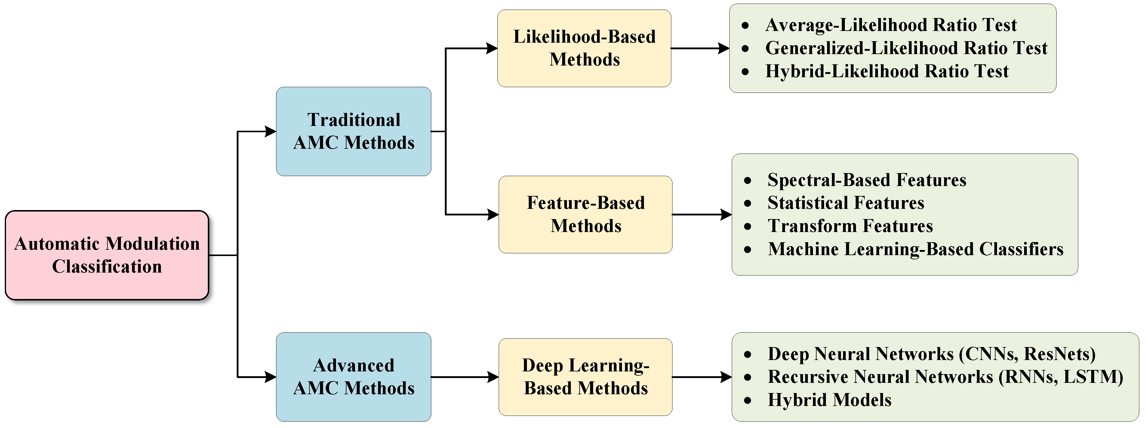
:1. Introduction
2. Signal Model and Proposed Classification Method
2.1. Signal Model
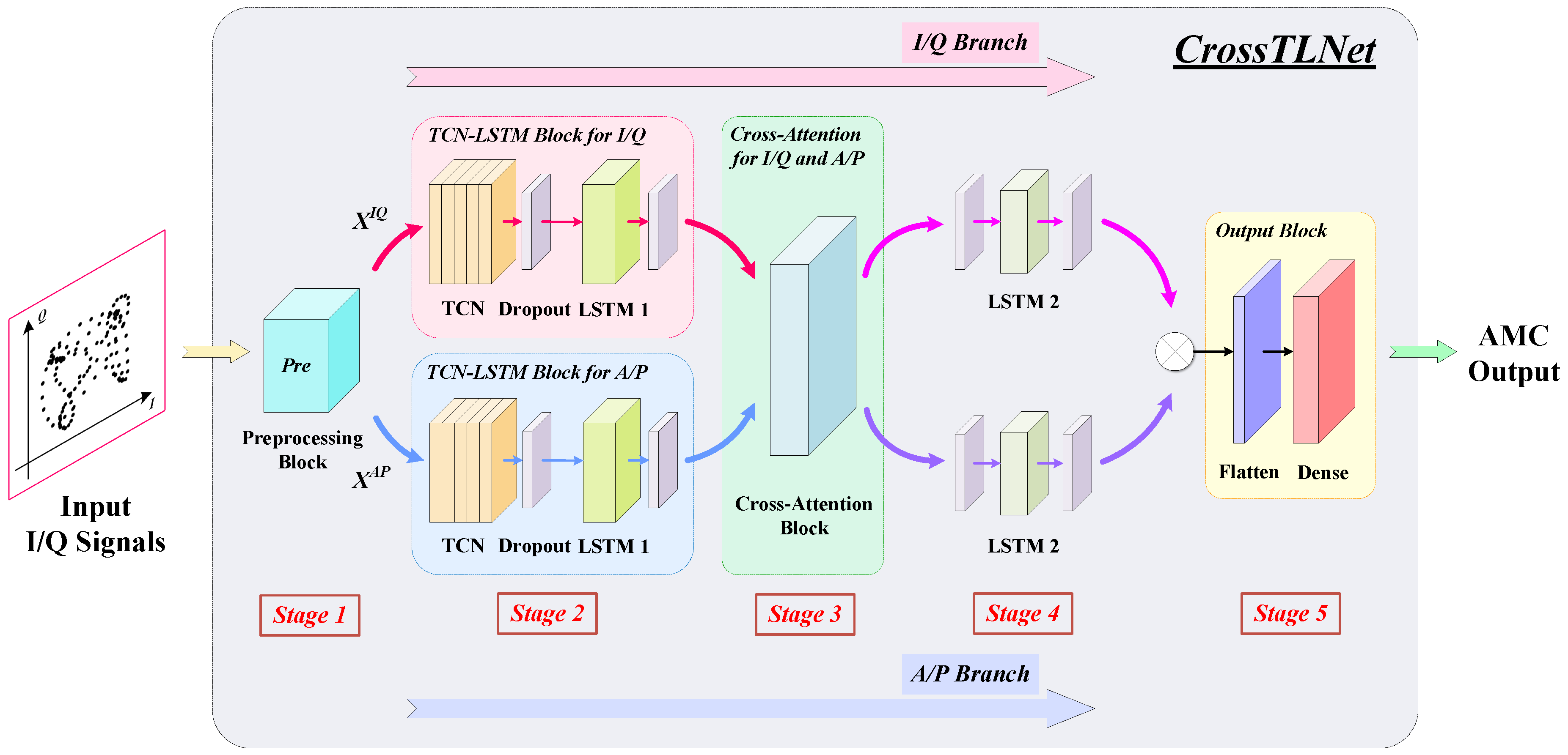
2.2. The Framework of CrossTLNet
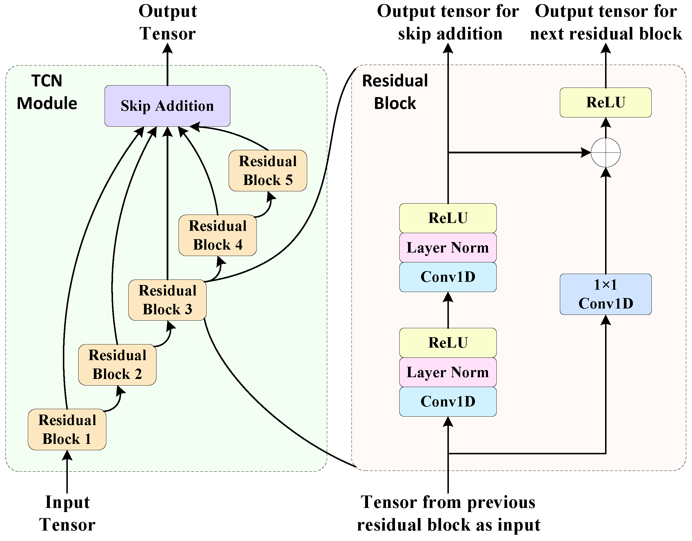
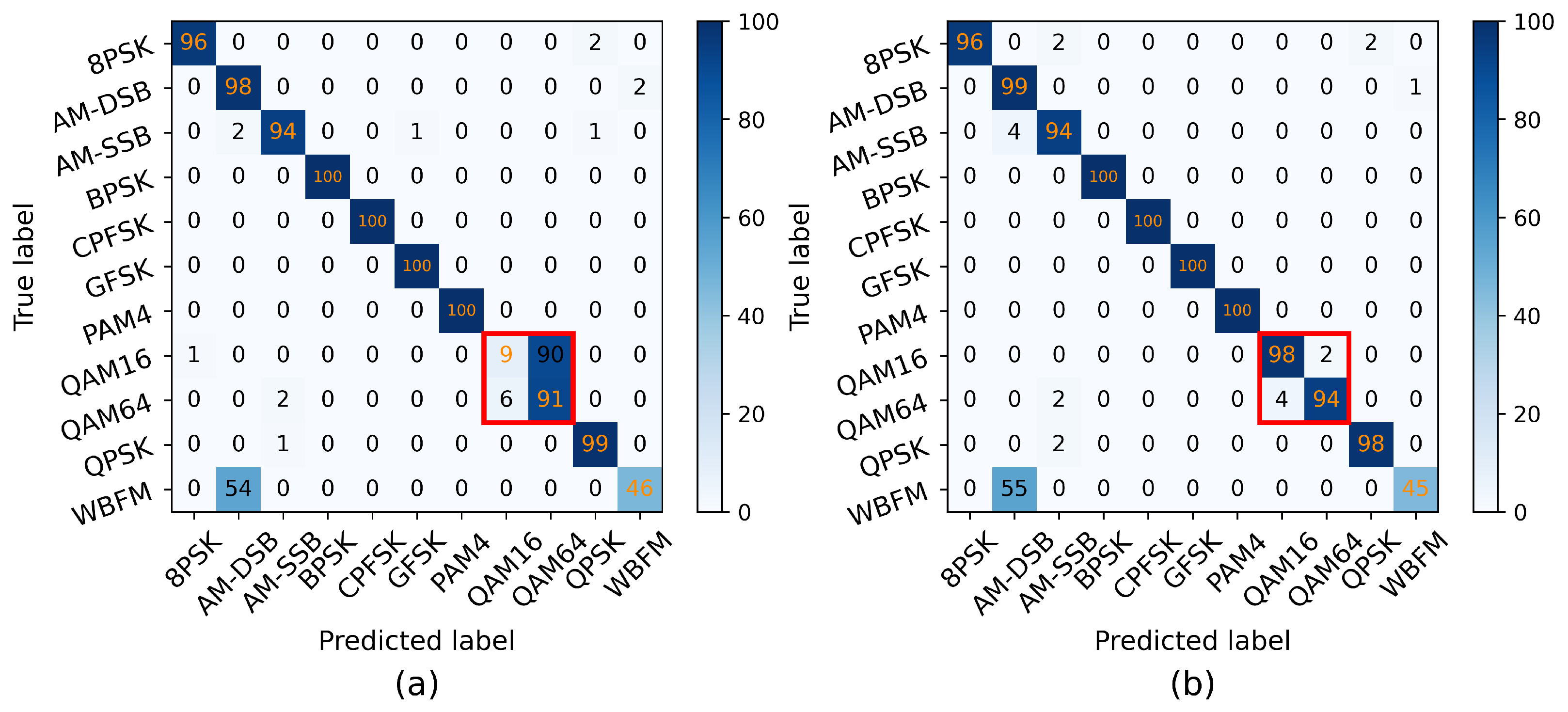
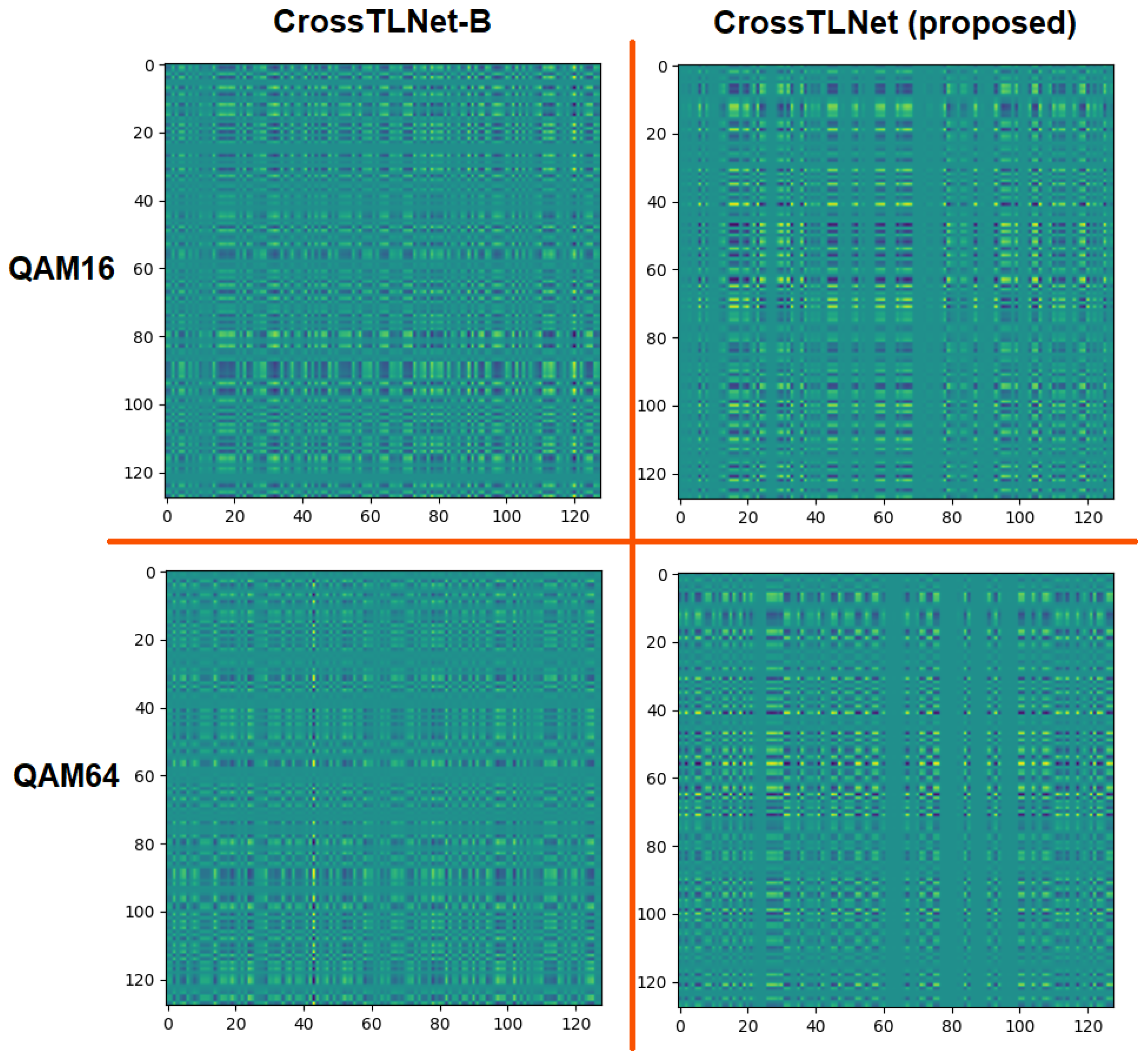
2.3. The Method with TCN–LSTM for High-Order Modulations
2.4. The Method of Cross-Attention
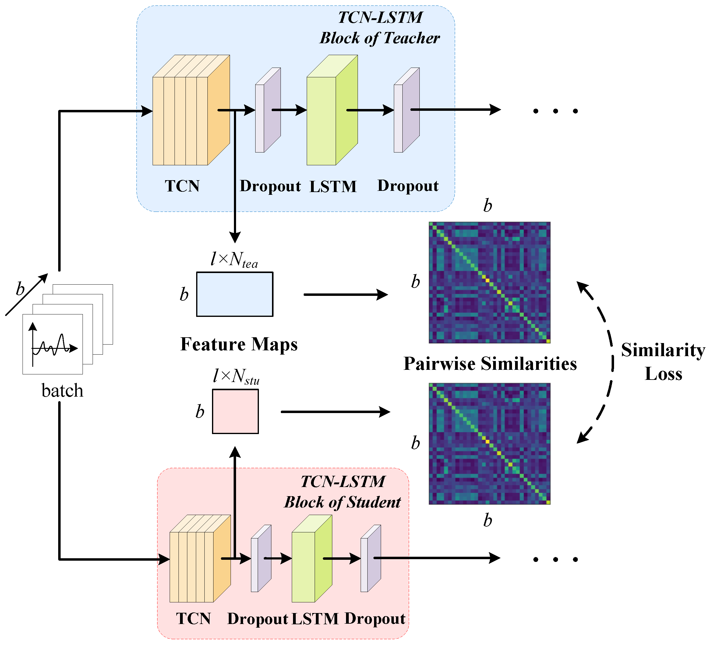
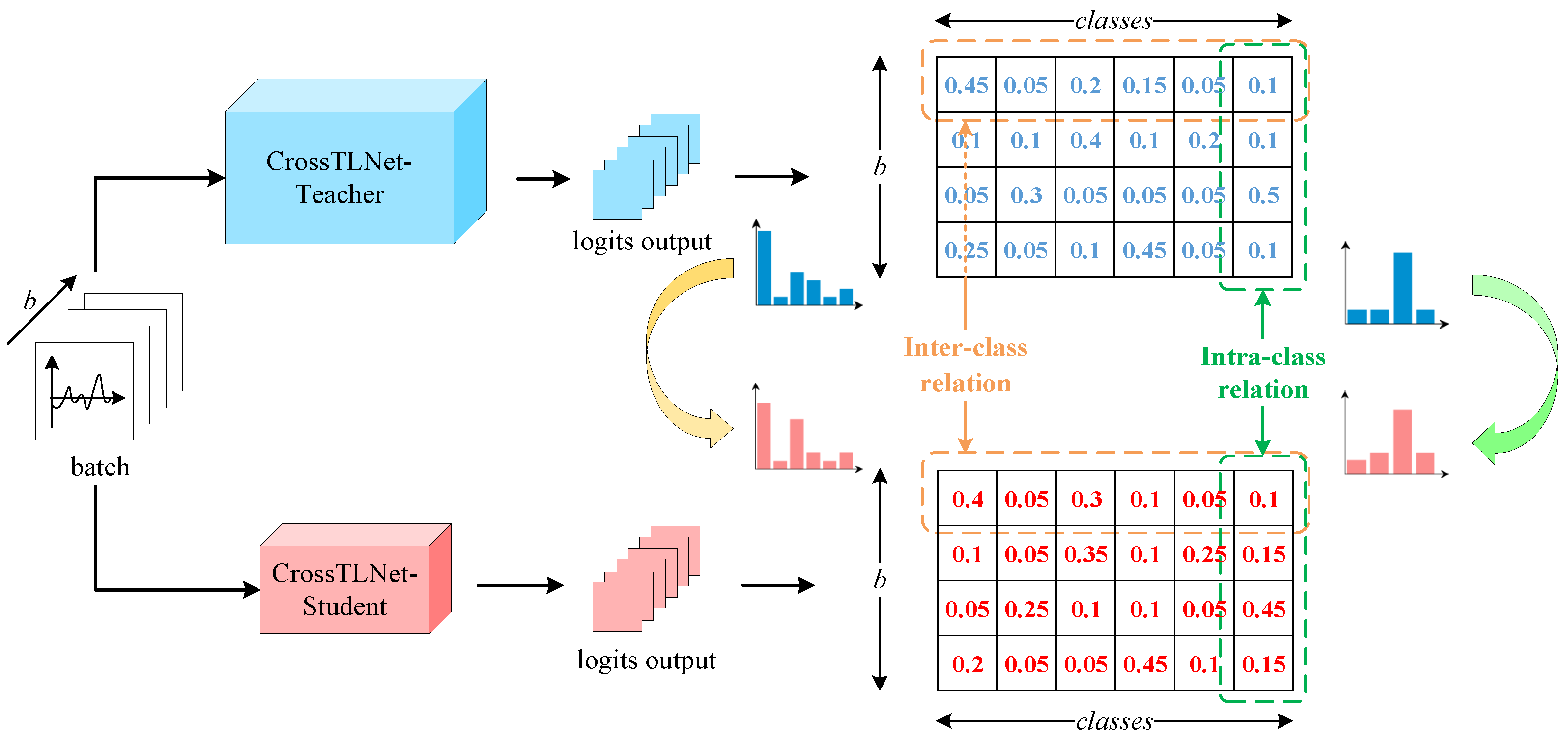
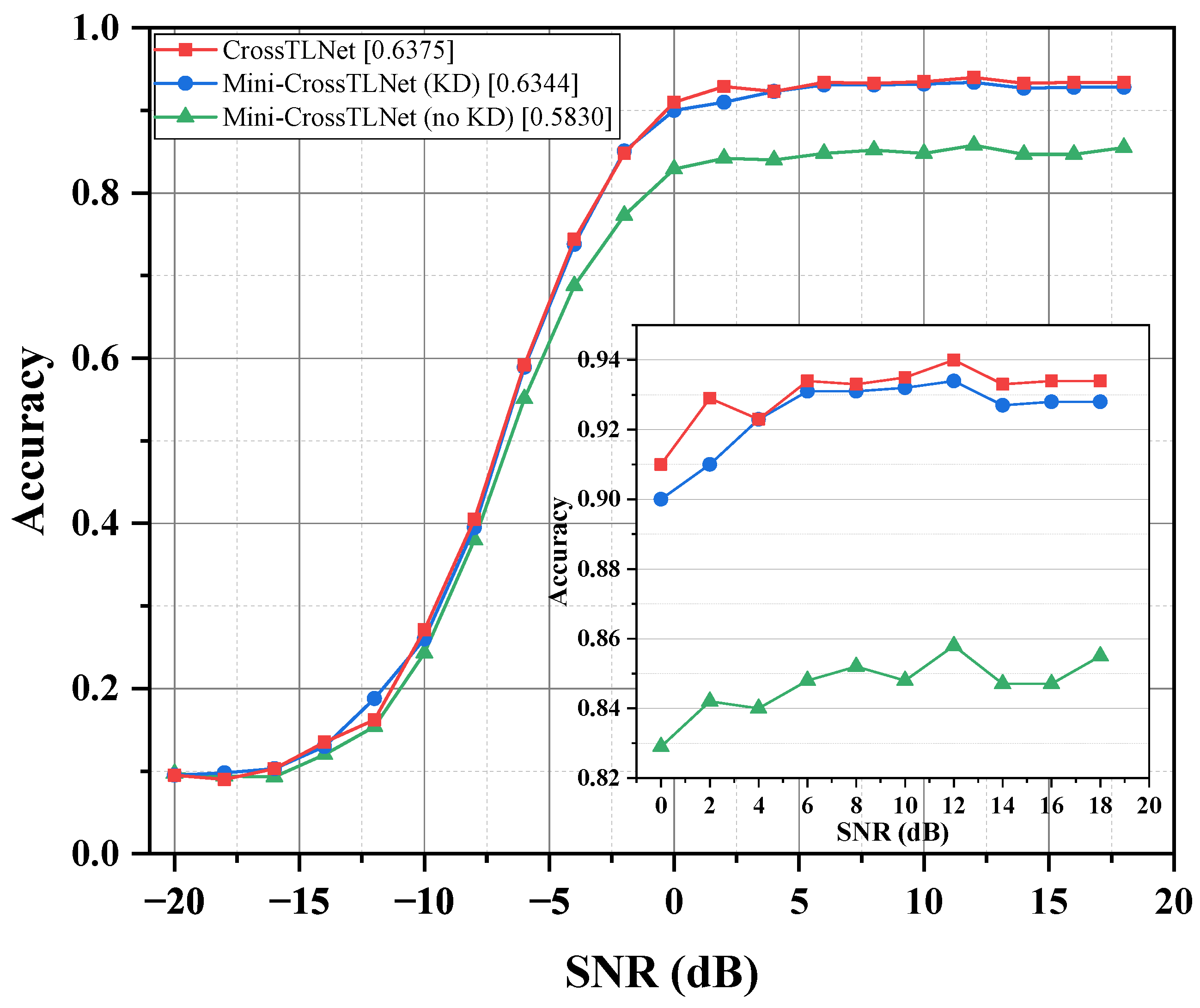
2.5. The Method of Model Lightweighting
- The part of feature-based knowledge distillation.
- The part of logits-based knowledge distillation
3. Experiments and Results Analysis
3.1. Dataset and Training Setting
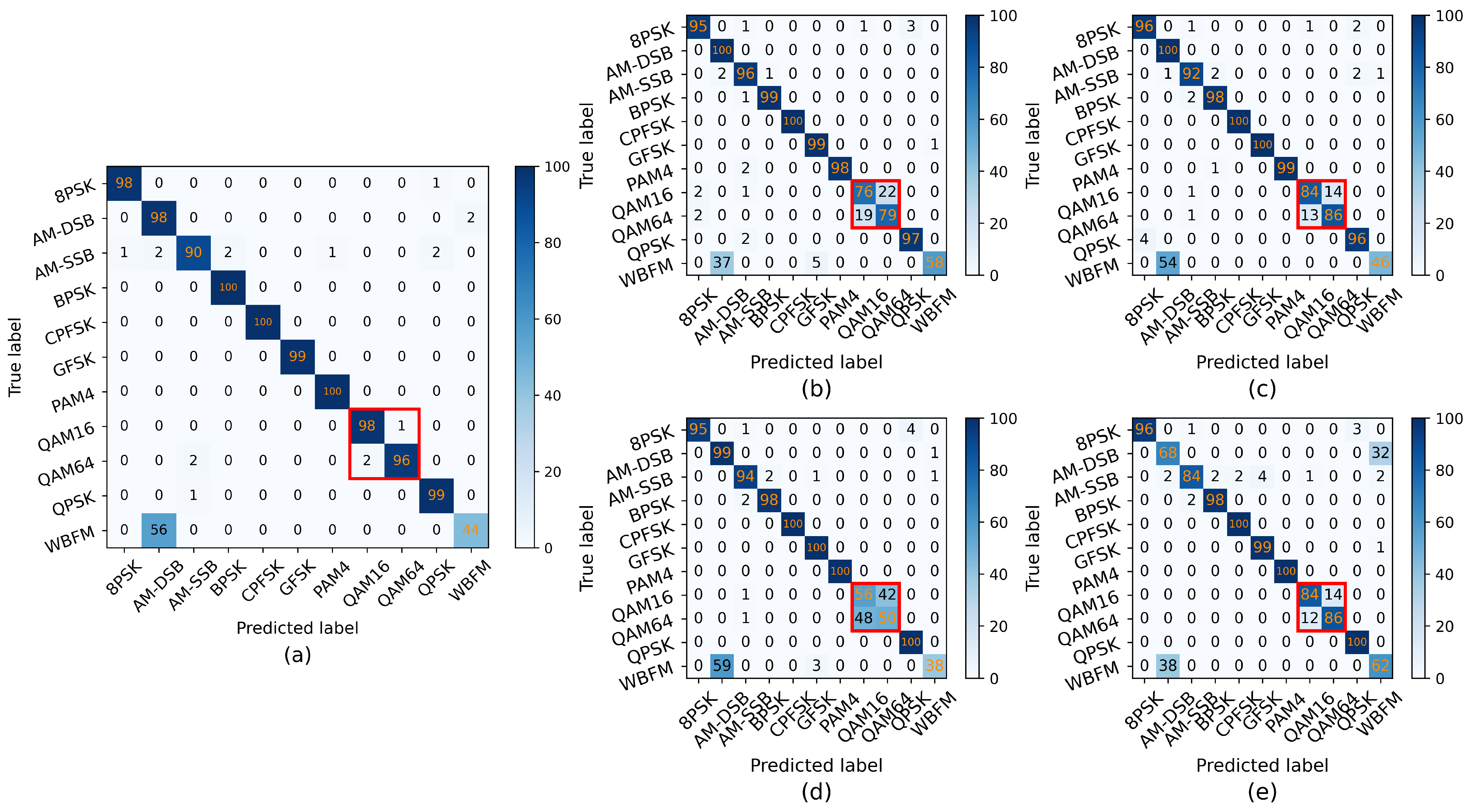
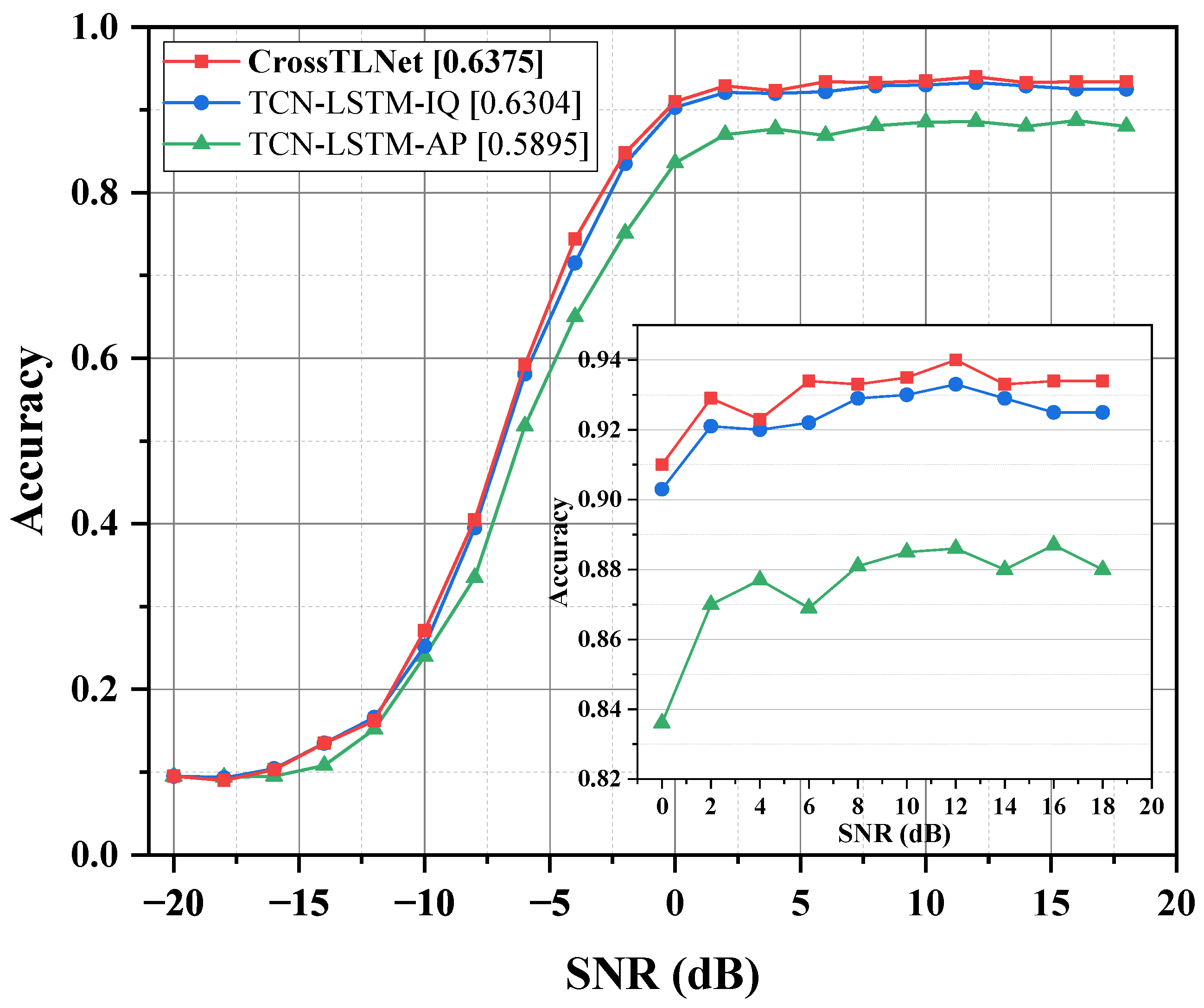
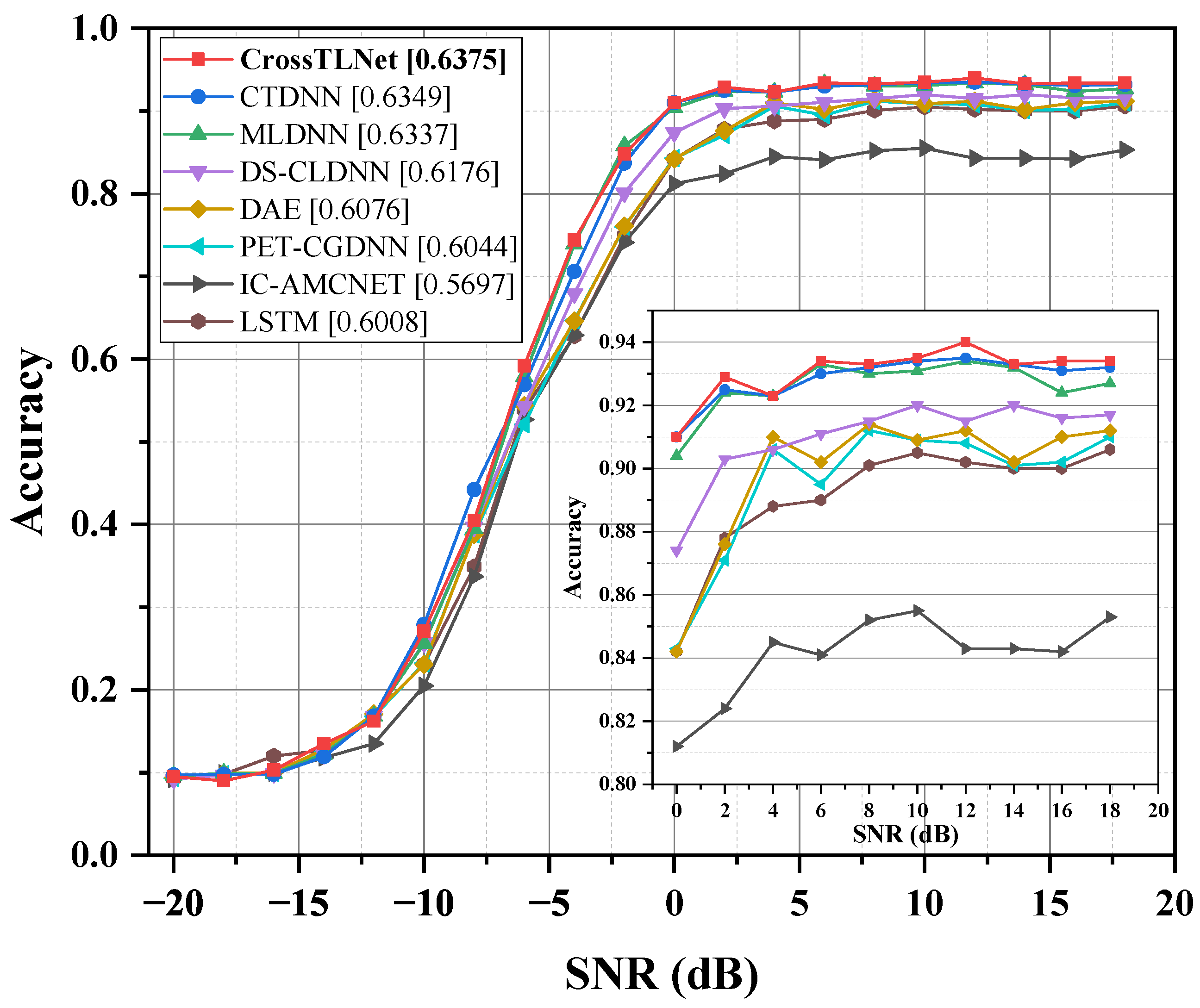
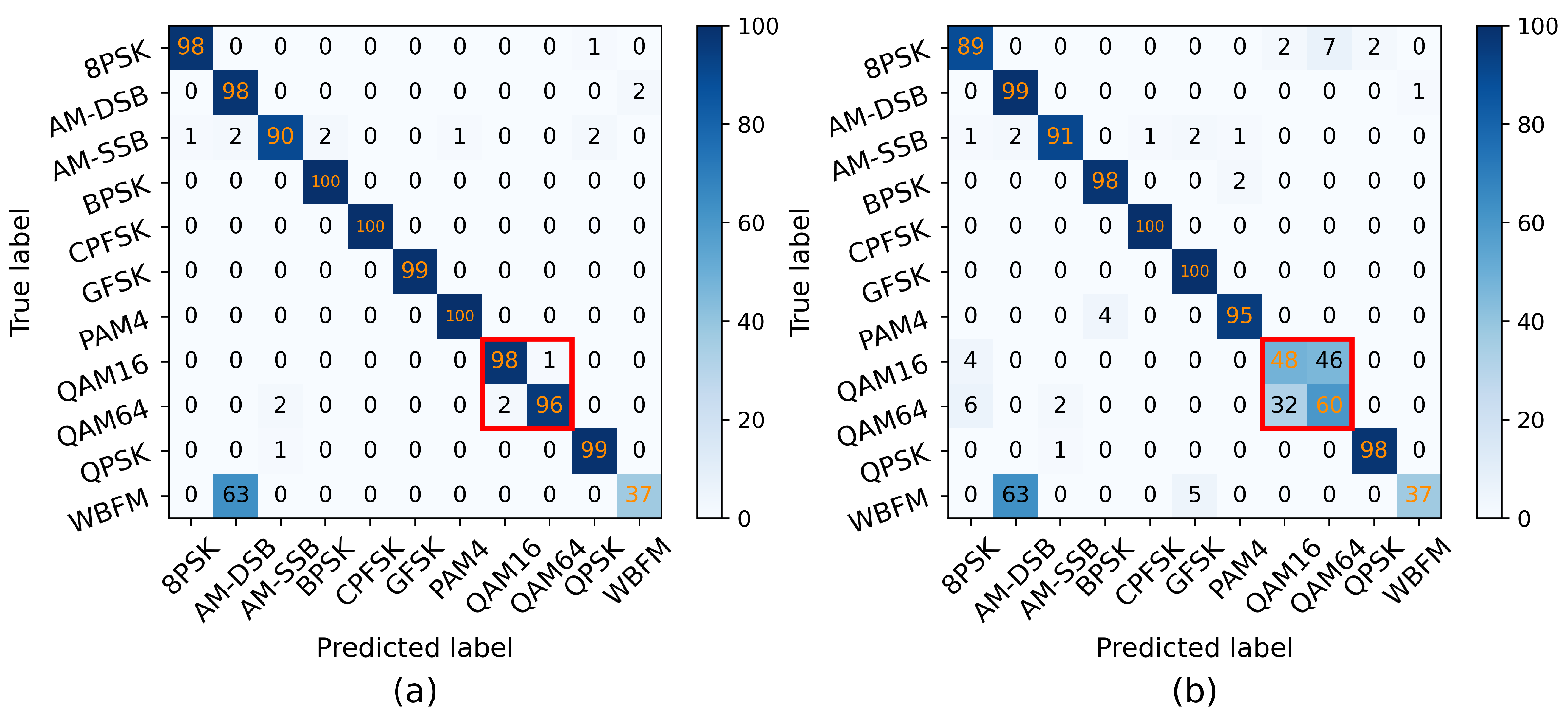
3.2. Results and Discussion
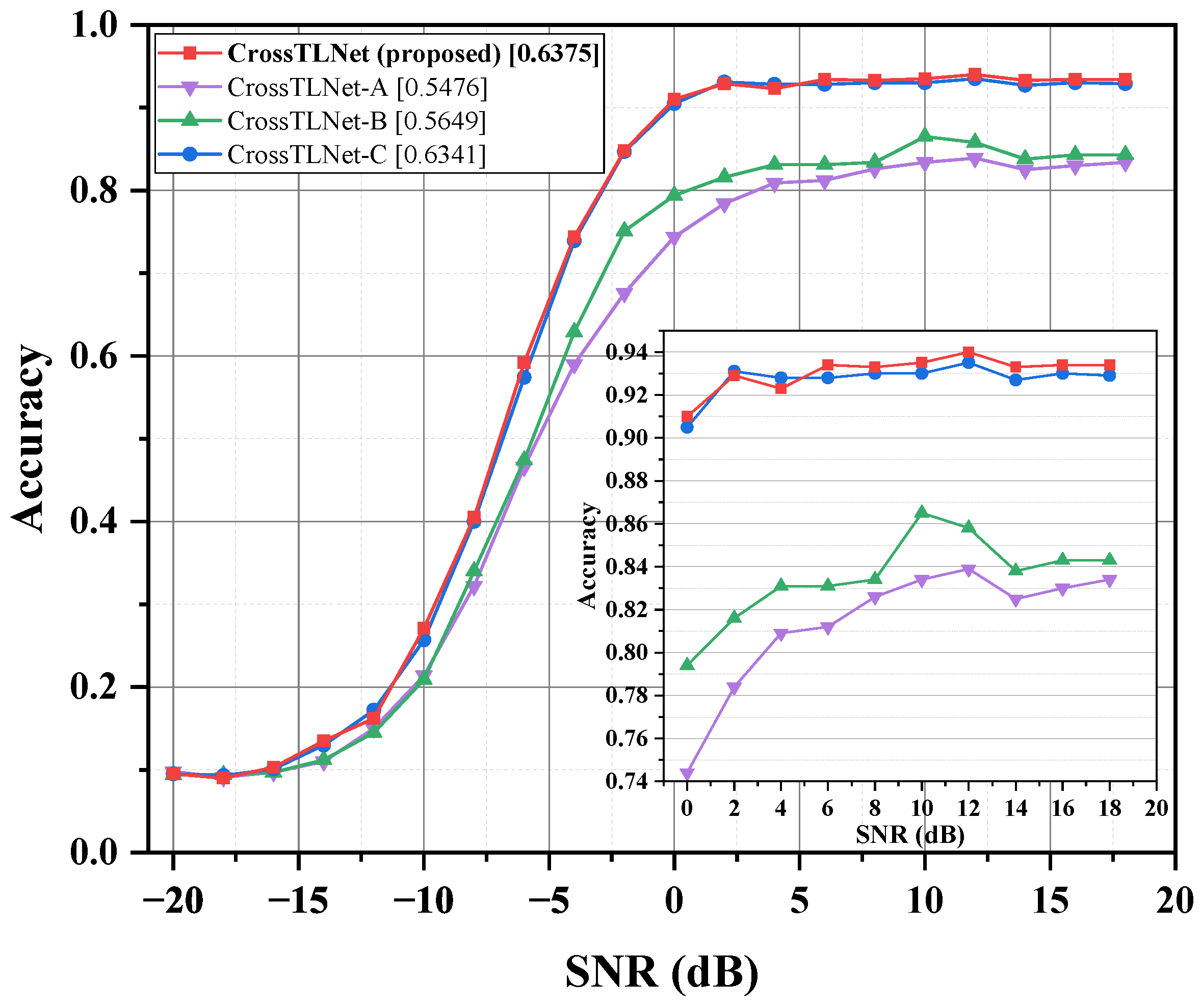
3.3. Ablation Study
3.4. Lightweight Model
4. Conclusions
Author Contributions
Funding
Data Availability Statement
Conflicts of Interest
References
- Wang, Y.; Wang, J.; Zhang, W.; Yang, J.; Gui, G. Deep learning-based cooperative automatic modulation classification method for MIMO systems. IEEE Trans. Veh. Technol. 2020, 69, 4575–4579. [Google Scholar] [CrossRef]
- O’Shea, T.J.; Corgan, J.; Clancy, T.C. Convolutional radio modulation recognition networks. In Proceedings of the Engineering Applications of Neural Networks: 17th International Conference, Aberdeen, UK, 2–5 September 2016; pp. 213–226. [Google Scholar] [CrossRef]
- Liu, X.; Yang, D.; El Gamal, A. Deep neural network architectures for modulation classification. In Proceedings of the 51st Asilomar Conference on Signals, Systems, and Computers, Pacific Grove, CA, USA, 29 October–1 November 2017; pp. 915–919. [Google Scholar] [CrossRef]
- Rajendran, S.; Meert, W.; Giustiniano, D.; Lenders, V.; Pollin, S. Deep learning models for wireless signal classification with distributed low-cost spectrum sensors. IEEE Trans. Cogn. Commun. Netw. 2018, 4, 433–445. [Google Scholar] [CrossRef]
- Zhang, F.; Luo, C.; Xu, J.; Luo, Y. An efficient deep learning model for automatic modulation recognition based on parameter estimation and transformation. IEEE Commun. Lett. 2021, 25, 3287–3290. [Google Scholar] [CrossRef]
- Zhang, Z.; Luo, H.; Wang, C.; Gan, C.; Xiang, Y. Automatic modulation classification using CNN–LSTM based dual-stream structure. IEEE Trans. Veh. Technol. 2020, 69, 13521–13531. [Google Scholar] [CrossRef]
- Wang, M.; Fan, Y.; Fang, S.; Cui, T.; Cheng, D. A Joint Automatic Modulation Classification Scheme in Spatial Cognitive Communication. Sensors 2022, 22, 6500. [Google Scholar] [CrossRef] [PubMed]
- Chang, S.; Huang, S.; Zhang, R.; Feng, Z.; Liu, L. Multitask-learning-based deep neural network for automatic modulation classification. IEEE Internet Things J. 2021, 9, 2192–2206. [Google Scholar] [CrossRef]
- Ying, S.; Huang, S.; Chang, S.; Yang, Z.; Feng, Z.; Guo, N. A convolutional and transformer based deep neural network for automatic modulation classification. China Commun. 2023, 20, 135–147. [Google Scholar] [CrossRef]
- Bai, S.; Kolter, J.Z.; Koltun, V. An empirical evaluation of generic convolutional and recurrent networks for sequence modeling. arXiv 2018, arXiv:1803.01271. [Google Scholar] [CrossRef]
- Vaswani, A.; Shazeer, N.; Parmar, N.; Uszkoreit, J.; Jones, L.; Gomez, A.N.; Kaiser, Ł.; Polosukhin, I. Attention is all you need. Adv. Neural Inf. Process. Syst. 2017, 30, 6000–6010. [Google Scholar] [CrossRef]
- Hinton, G.; Vinyals, O.; Dean, J. Distilling the knowledge in a neural network. arXiv 2015, arXiv:1503.02531. [Google Scholar] [CrossRef]
- Tung, F.; Mori, G. Similarity-preserving knowledge distillation. In Proceedings of the IEEE/CVF International Conference on Computer Vision, Seoul, Republic of Korea, 27 October–2 November 2019; pp. 1365–1374. [Google Scholar] [CrossRef]
- Huang, T.; You, S.; Wang, F.; Qian, C.; Xu, C. Knowledge distillation from a stronger teacher. Adv. Neural Inf. Process. Syst. 2022, 35, 33716–33727. [Google Scholar] [CrossRef]
- DeepSig Team. RF Datasets For Machine Learning. Available online: https://opendata.deepsig.io/datasets/2016.10/RML2016.10a.tar.bz2 (accessed on 1 November 2023).
- Zhang, F.; Luo, C.; Xu, J.; Luo, Y.; Zheng, F.C. Deep learning based automatic modulation recognition: Models, datasets, and challenges. Digit. Signal Process. 2022, 129, 103650. [Google Scholar] [CrossRef]
- O’shea, T.; Hoydis, J. An introduction to deep learning for the physical layer. IEEE Trans. Cogn. Commun. Netw. 2017, 3, 563–575. [Google Scholar] [CrossRef]


| Author | Year | Model | Dataset | Input Signal | Main Structure of the Model |
|---|---|---|---|---|---|
| O’Shea et al. [2] | 2016 | CNN | RML | I/Q | CNN |
| Liu et al. [3] | 2017 | ResNet | RML | I/Q | ResNet |
| Rajendran et al. [4] | 2018 | LSTM | RML | A/P | Two LSTM Layers |
| Zhang et al. [5] | 2021 | PET-CGDNN | RML | I/Q | CNN + GRU + DNN |
| Zhang et al. [6] | 2020 | DS-CLDNN | RML | I/Q + A/P | CNN + LSTM |
| Wang et al. [7] | 2022 | IQCLNet | RML | I/Q | CNN + LSTM + Expert Feature Method for QAMs |
| Chang et al. [8] | 2021 | MLDNN | RML | I/Q + A/P | CNN + BiGRU + SAFN |
| Ying et al. [9] | 2023 | CTDNN | RML | I/Q | CNN + Transformer |
| Parameter Name | Value |
|---|---|
| Sampling frequency | 200 KHz |
| Sampling rate offset standard deviation | 0.01 Hz |
| Maximum sampling rate offset | 50 Hz |
| Carrier frequency offset standard deviation | 0.01 Hz |
| Maximum carrier frequency offset | 500 Hz |
| Number of sinusoids used in frequency selective fading | 8 |
| Maximum doppler frequency used in fading | 1 |
| Fading model | Rician |
| Rician K-factor | 4 |
| Fractional sample delays for the power delay profile | [0.0, 0.9, 1.7] |
| Magnitudes corresponding to each delay time | [1, 0.8, 0.3] |
| Filter length to interpolate the power delay profile | 8 |
| Standard deviation of the AWGN process |
| Hyperparameter Name | Value |
|---|---|
| Optimizer | Adam |
| Initial learning rate | 0.0001 |
| Batch size | 32 |
| Early-stop patience | 25 |
| Training–validation–testing ratio of dataset | 0.6:0.2:0.2 |
| Model | Accuracy | Accuracy () |
|---|---|---|
| CrossTLNet-128 | 0.6326 | 0.9221 |
| CrossTLNet-192 | 0.6360 | 0.9263 |
| CrossTLNet-256 (proposed) | 0.6375 | 0.9305 |
| CrossTLNet-320 | 0.6354 | 0.9264 |
| Model | TCN Module | Cross-Attention | Accuracy | Accuracy () |
|---|---|---|---|---|
| CrossTLNet-A | 0.5476 | 0.8137 | ||
| CrossTLNet-B | ✓ | 0.5649 | 0.8353 | |
| CrossTLNet-C | ✓ | 0.6341 | 0.9273 | |
| CrossTLNet (proposed) | ✓ | ✓ | 0.6375 | 0.9305 |
| Model | Parameters | Accuracy |
|---|---|---|
| CrossTLNet | 6760.5 K | 0.6375 |
| Mini-CrossTLNet (KD) | 575.0 K | 0.6344 |
| CTDNN | 2577.2 K | 0.6349 |
| MLDNN | 899.25 K | 0.6337 |
| DS-CLDNN | 1144.7 K | 0.6176 |
Disclaimer/Publisher’s Note: The statements, opinions and data contained in all publications are solely those of the individual author(s) and contributor(s) and not of MDPI and/or the editor(s). MDPI and/or the editor(s) disclaim responsibility for any injury to people or property resulting from any ideas, methods, instructions or products referred to in the content. |
© 2023 by the authors. Licensee MDPI, Basel, Switzerland. This article is an open access article distributed under the terms and conditions of the Creative Commons Attribution (CC BY) license (https://creativecommons.org/licenses/by/4.0/).
Share and Cite
Gao, G.; Hu, X.; Li, B.; Wang, W.; Ghannouchi, F.M. CrossTLNet: A Multitask-Learning-Empowered Neural Network with Temporal Convolutional Network–Long Short-Term Memory for Automatic Modulation Classification. Electronics 2023, 12, 4668. https://doi.org/10.3390/electronics12224668
Gao G, Hu X, Li B, Wang W, Ghannouchi FM. CrossTLNet: A Multitask-Learning-Empowered Neural Network with Temporal Convolutional Network–Long Short-Term Memory for Automatic Modulation Classification. Electronics. 2023; 12(22):4668. https://doi.org/10.3390/electronics12224668
Chicago/Turabian StyleGao, Gujiuxiang, Xin Hu, Boyan Li, Weidong Wang, and Fadhel M. Ghannouchi. 2023. "CrossTLNet: A Multitask-Learning-Empowered Neural Network with Temporal Convolutional Network–Long Short-Term Memory for Automatic Modulation Classification" Electronics 12, no. 22: 4668. https://doi.org/10.3390/electronics12224668
APA StyleGao, G., Hu, X., Li, B., Wang, W., & Ghannouchi, F. M. (2023). CrossTLNet: A Multitask-Learning-Empowered Neural Network with Temporal Convolutional Network–Long Short-Term Memory for Automatic Modulation Classification. Electronics, 12(22), 4668. https://doi.org/10.3390/electronics12224668