Deep-Reinforcement-Learning-Based Dynamic Ensemble Model for Stock Prediction

Abstract

In stock prediction problems, deep ensemble models are better adapted to dynamically changing stock market environments compared to single time-series networks. However, the existing ensemble models often underutilize real-time market feedback for effective supervision, and base models are pre-trained and fixed in their optimization, which makes them lack adaptability for evolving market environments. To address this issue, we propose a deep-reinforcement-learning-based dynamic ensemble model for stock prediction (DRL-DEM). Firstly, we employ deep reinforcement learning to optimize the weights of deep-learning-based time-series models. Secondly, existing deep-reinforcement-learning methods only consider environmental rewards. Thus we improve the reward function by introducing real-time investment returns as additional feedback signals for the deep-reinforcement-learning algorithm. Finally, an alternating iterative algorithm is used to simultaneously train the base predictors and the deep-reinforcement-learning model, allowing DRL-DEM to fully utilize the supervised information for global coordinated optimization. The experimental results show that in SSE 50 and NASDAQ 100 datasets, the mean square error (MSE) of the proposed method reached 0.011 and 0.005, the Sharpe ratio (SR) reached 2.20 and 1.53, and the cumulative return (CR) reached 1.38 and 1.21. Compared with the best results in the recent model, MSE decreased by 21.4% and 28.6%, SR increased by 81.8% and 82.1%, and CR increased by 89.0% and 89.1%, with higher forecasting accuracy and stronger investment return capability.

1. Introduction

Stock investment holds a significant place in the realm of financial investments. In the process of stock investment, accurate stock prediction plays a decisive role in constructing investment decisions and risk hedging [1]. Traditional stock prediction methods primarily rely on statistical methods, such as autoregressive integrated moving average (ARIMA) [2], vector autoregressive (VAR) [3], etc. However, in a large number of practical applications, the complex nonlinear characteristics of stock data make these traditional models unable to achieve accurate predictions. With the rapid advancement in computer technology, deep learning is gradually being applied to stock price prediction [4,5,6], including long short-term memory (LSTM) networks [7], gated recurrent unit (GRU) networks [8], LSTM neural networks with attention mechanisms [9] (ALSTM) [10], and Transformers [11], etc. These networks possess the ability to learn long-term dependencies, capture short-term features, and effectively model complex nonlinear patterns in stock data.

However, due to the increasingly complex stock data environment, it is becoming more and more challenging to make high-precision predictions using traditional single prediction models. Makridakis et al. [12] demonstrates that ensemble methods can enhance prediction accuracy and improve model stability by leveraging the strengths of individual models. Nevertheless, the performance of an ensemble prediction model is primarily influenced by the weight distribution of its base models, and finding the optimal weight distribution method remains a challenging problem [13,14]. Traditional ensemble methods [15,16] often overlook variations in predictive performance among different models, limiting the potential benefits of ensemble learning. Zhao et al. [17] evaluated the predictive performance of each base model through in-sample testing and calculated the weight of each model. They then used these weights to train the model for weight prediction, and finally, calculated a weighted average to obtain the ensemble result. Nti et al. [18] combined ensemble learning with a genetic algorithm and performed feature selection and parameter optimization simultaneously. Sun et al. [19] employed the adaptive enhanced regression algorithm to iteratively train and ensemble multiple LSTM models for stock index prediction. While the above methods do improve the accuracy of inventory forecasting to varying degrees, there is still room for further improvement in terms of time complexity. Fu et al. [20] proposed a dynamic time-series prediction ensemble model based on deep reinforcement learning (RLMC). This approach uses deep reinforcement learning to train an agent to automatically perform optimal selection and a combination of multiple prediction models, thereby enabling dynamic adaptation and optimization of prediction. By using deep reinforcement learning to output continuous actions to solve the model combination weight problem, the time complexity can be significantly reduced compared to discrete weight selection in traditional methods. In addition, compared with genetic algorithms and adaptive enhanced regression algorithms, the experience replay technology in deep reinforcement learning enables the storage and reuse of large amounts of historical data. Reusing historical data can greatly reduce the amount of training samples required, improve sample efficiency, and reduce the time complexity of each iteration.

Although deep reinforcement learning can effectively explore the optimal weight distribution of different models and realize the efficient ensemble of multiple models [21], its application in the field of stock prediction is not extensive. To better adapt deep-reinforcement-learning ensemble methods to the complexity and dynamics of the stock market, there are still two challenges that need to be addressed in existing methods. On one hand, current deep-reinforcement-learning ensemble models rely solely on environmental rewards, which may lead the model’s behavior to converge to local optima, preventing it from achieving a global optimum. On the other hand, the base predictor in the ensemble model is typically treated as a fixed component and does not participate in the model’s update process. For example, in the dynamic time-series prediction ensemble model based on deep reinforcement learning proposed in [20], the base predictor will not participate in the update during the training of deep reinforcement learning after the initial advance training is completed, and is a fixed component. This limits the flexibility and adaptability of the model to a certain extent. In response to these issues, this paper proposes a deep-reinforcement-learning-based dynamic ensemble model for stock prediction (DRL-DEM). The main contributions are as follows:

• Our framework constructs base predictors of different prediction styles by selecting different neural network structures (such as GRU, ALSTM, and Transformer), loss functions, and the number of hidden layers to cope with the complex and ever-changing stock market. Furthermore, we use deep reinforcement learning to explore the optimal weight allocation of base predictors, converting the problem of optimal configuration of base predictor weights into a deep-reinforcement-learning task.
• Improving the design of only environmental rewards in the return function of the existing deep-reinforcement-learning algorithm, and introducing real-time investment income as an additional feedback signal to the deep-reinforcement-learning algorithm. By constructing a hybrid reward function, our DRL-DEM can maximize investment return.
• Using an iterative algorithm to simultaneously train the base predictors and deep-reinforcement learning. DRL-DEM optimize the weight of the ensemble model and update the network parameters of the base predictor at the same time, so that the base predictors can be adaptively adjusted to the feedback signal, and we realize the global collaboration of the ensemble model optimization to improve the prediction accuracy of the model.

2. Related Work

2.1. Stock Prediction Based on Deep Learning

Stock prediction is a crucial research area within the financial domain. Traditional stock prediction models primarily rely on statistical methods [22,23], but their performance on complex nonlinear data fitting is often limited. Some machine learning methods like support vector machines [24], decision trees [25], etc., have emerged to perform nonlinear mapping on data, enhancing their fitting capabilities. They can also gradually approach the target through segmentation rules. However, these methods have certain limitations when addressing high-dimensional complex problems.

Deep learning is highly effective at processing high-dimensional and complex market data; it can automatically learn key features and complex nonlinear relationships hidden within the data [26,27]. Gao et al. [28] employed deep learning methods to reduce the dimensionality and perform feature selection on multiple factors influencing stock prices, comparing the performance of algorithms such as LSTM and GRU. Experiments demonstrated that this approach yields improved stock price predictions. Li et al. [29] introduced a multi-input structure and a two-layer attention mechanism into the LSTM model, enabling the distinction between primary factors and auxiliary factors. They also incorporated related stocks of the target stock as auxiliary predictors. Yoo et al. [30] proposed the data-axis transformer with multi-level contexts (DTML) model. This end-to-end model employs temporal attention to extract stock features, incorporates market indices as global features, and leverages the Transformer architecture to learn feature associations. Compared to traditional methods, the aforementioned deep-learning-based stock prediction models excel in capturing complex market characteristics, enhancing prediction accuracy, and improving interpretability. However, in a dynamic stock market environment, a single prediction model may struggle to fully account for various uncertain factors, and a model’s stability cannot be guaranteed entirely. Therefore, this paper aims to ensemble a variety of deep-learning-based time-series prediction models, harnessing the strengths of each model to achieve a more accurate and stable stock prediction.

2.2. Ensemble Methods Based on Deep Reinforcement Learning

Traditional methods for a model ensemble primarily rely on expert rules and meta-learning. Collopy et al. [31] used an expert system method for model combination. However, the subjectivity and uncertainty in manually setting the weight assignment rules may negatively affect the model. Talagala et al. [32] introduced meta-learning to formulate the model selection task as a classification problem. Montero-Manso et al. [33] selected weights for weighted prediction combinations via meta-learning. However, this method only uses the attribute characteristics of the time series to determine the weight coefficient of the model at one time, which cannot be well adapted to the dynamic environment.

With the rapid advancement of machine learning, some studies have started using reinforcement learning to address the problem of ensemble model weighting. Feng et al. [34] introduced a method employing Q-learning agents to tackle model selection, but it requires learning a large number of weights for each rolling window. Saadallah et al. [35] proposed an ensemble prediction framework based on the actor-critic algorithm, dynamically optimizing the weight combination strategy through continuous actor learning. Fu et al. [20] incorporated deep reinforcement learning to dynamically determine the weights of ensemble models in time-series prediction tasks, achieving superior prediction results across multiple time-series datasets. However, deep-reinforcement-learning-based ensemble methods have not yet been widely used for stock ensemble prediction. Furthermore, in the face of complex stock market environments, existing deep-reinforcement-learning ensemble algorithms rely solely on environmental rewards, which leads to models being confined to local optima and failing to achieve optimal performance. In most cases, the base predictor in ensemble models is treated as a fixed component and does not actively participate in the model’s update process. This limits the flexibility, adaptability, and learning capacity of the ensemble model. To better adapt to the complex and dynamically changing stock market environment and achieve the goal of high-precision prediction and maximized investment returns, this paper introduces real-time investment returns as an additional feedback signal to the deep-reinforcement-learning algorithm. An alternate iterative algorithm is employed for simultaneous training of base predictors and deep reinforcement learning, enabling global co-optimization of the ensemble model.

Table 1. Summary of related work.

Method	Ensemble/ Non-Ensemble	Applied Models	Source of Dataset	Performance Metrics
SVM [24]	Non-Ensemble	SVM	NASDAQ Index	Accuracy
DTML [30]	Non-Ensemble	ALSTM, Transformer	NDX100, CSI300, etc.	Accuracy, MCC
CNN-LSTM [26]	Non-Ensemble	CNN, LSTM	Shanghai Composite Index	RMSE, MAE, $R^2$
ABC-LSTM [27]	Non-Ensemble	ABC, LSTM	AAPL, AMZN, INFY, TCS, ORCL, and MSFT	MAPE, MSE, etc.
GASVM [18]	Ensemble	SVM, GA	Banks and oil company stocks on the GSE	Accuracy, RMSE etc.
LSTM-AdaBoost.R2 [19]	Ensemble	LST, AdaBoost.R2	SSEC, CSI300, and SZSC	RMSE, MAPE
RLMC [20]	Ensemble	GRU, LSTM, dialated CNN etc., DRL	ETT, Climate, etc.	MAE, sMAPE
OEA-RL [35]	Ensemble	ARIMA, ETS etc.; DRL	Meteorological data, Water resources data, etc.	Avg. Rank

ABC: Artificial Bee Colony, GA: Genetic Algorithm, GSE: Ghana Stock Exchange, DRL: Deep Reinforcement Learning, ETS: Exponential Smoothing.

provides an overview of the main findings in related research. To address the challenges present in the field of stock ensemble forecasting and better adapt to the complexity and dynamics of the stock market, this study introduces a deep-reinforcement-learning-based ensemble model for dynamic stock prediction.

3. DRL-DEM Structure

3.1. Definition of the Problem

In this paper, the problem of the optimal allocation of base predictor weights is transformed into a deep-reinforcement-learning task to optimize investment decisions. Specifically, we use stock data as the input for the base predictor. The deep-reinforcement-learning algorithm comprehensively considers the output of the base predictor, historical performance, and real-time market investment feedback, and dynamically adjusts the weight configuration of the base predictor to obtain the optimal ensemble prediction results and higher return on investment. The above process conforms to the Markov decision process (MDP). The MDP variables are defined as follows:

• $S=(s_1,s_2,\dots ,s_t,\dots )$ is the state space, the state $s_t$ describes the stock data $x_t\in R^{m\times k}$ at time t along with the historical losses of the base predictors $l_t\in R^{m\times n}$, where m represents the number of stocks, k represents the number of feature factors, and n represents the number of base predictors.
• $A=(a_1,a_2,\dots ,a_t,\dots )$ is the action space, and action $a_t\in R^{m\times n}$ describes the weights of n base predictors corresponding to m stocks at time t.
• $s_t$ is transformed into $s_{t+1}\sim P\left(s_{t+1}|s_t,a_t\right)=P\left(s_{t+1}|s_t\right)$ according to the transition distribution, and action $a_t$ does not affect the next state $s_{t+1}$.
• $R\left(s_t,a_t,s_{t+1}\right)$ represents the immediate reward generated by taking action $a_t$ in state $s_t$ and transitioning to the new state $s_{t+1}$.
• The discount factor $\gamma \in \left[0,1\right]$ describes the trade-off for future performance.

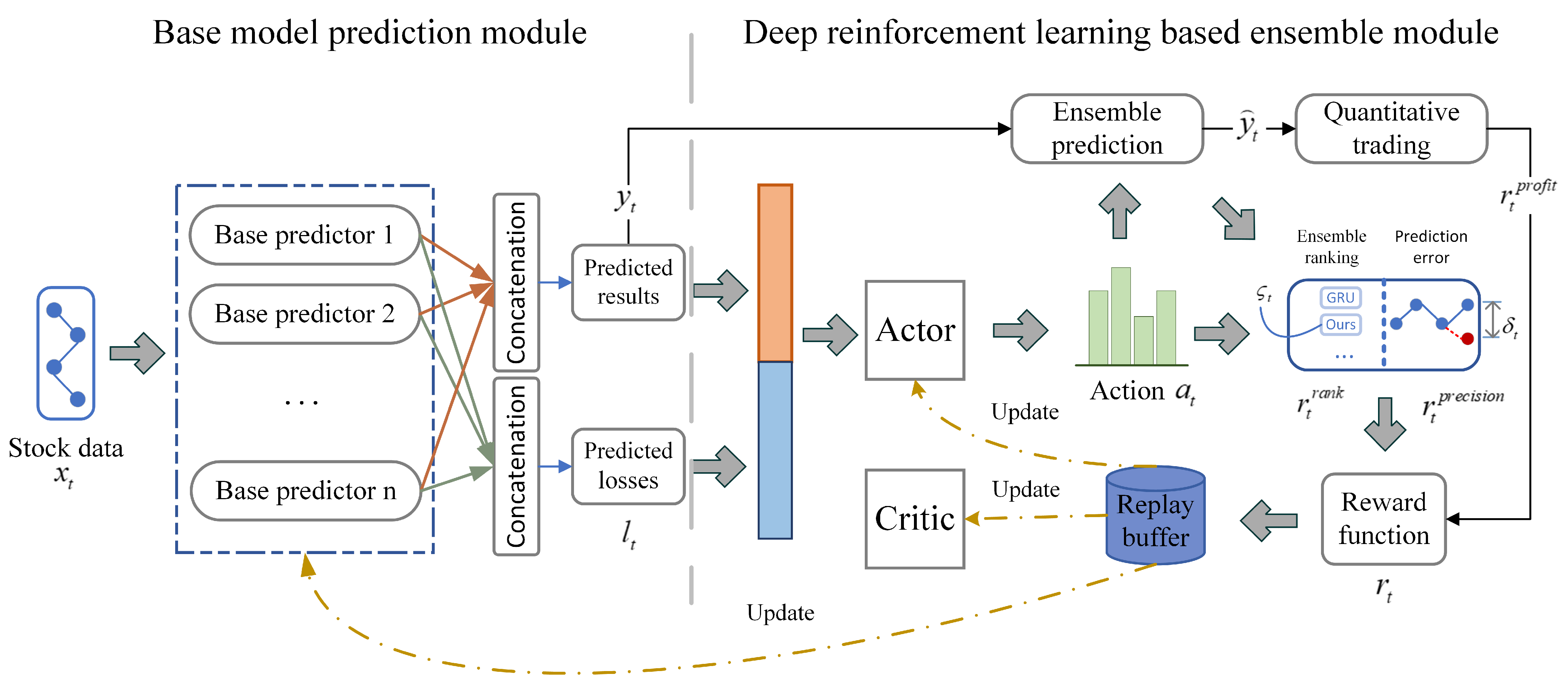
3.2. DRL-DEM Overall Framework

DRL-DEM introduces a stock dynamic prediction ensemble model based on deep reinforcement learning for investment trading. Figure 1 illustrates the overall model framework of the proposed approach.

First, n time-series prediction models with varying neural network structures (such as GRU, ALSTM, and Transformer), loss functions, and the number of hidden layers are selected as the base predictors for DRL-DEM to predict stock returns. At time t, the market data $x_t$ of m stocks is used as input for n base predictors, which then output the predicted income $y_t$ for the m stocks and the prediction errors $l_t$ for the n base predictors.

Second, the deep-reinforcement-learning-based ensemble model is used to optimize weights of base predictors. Taking $y_t$ and $l_t$ together as the input for the actor in the ensemble module, the actor’s output $a_t$ describes the weights assigned to n base predictors for the m stocks. Based on $a_t$ and $y_t$, the ensemble prediction ${\stackrel{⏜}{y}}_t$ of the stock is calculated. The top q stocks are selected from ${\stackrel{⏜}{y}}_t$, their predictions are normalized to determine the weights, and invested accordingly.

Then, after selecting an action $a_t$ in response to the state $s_t$, the actor network provides both $a_t$ and $s_t$ to the critic network. The critic network estimates $Q(s_t,a_t)$ and shares it with the actor network, which then updates its policy based on this feedback.

Finally, $\left(s_t,a_t,r_t,s_{t+1}\right)$ are placed into the replay experience pool. This allows the model to retrieve data from the replay experience pool in batches during the training process and update the parameters of the base predictor network, actor network, and critic network.

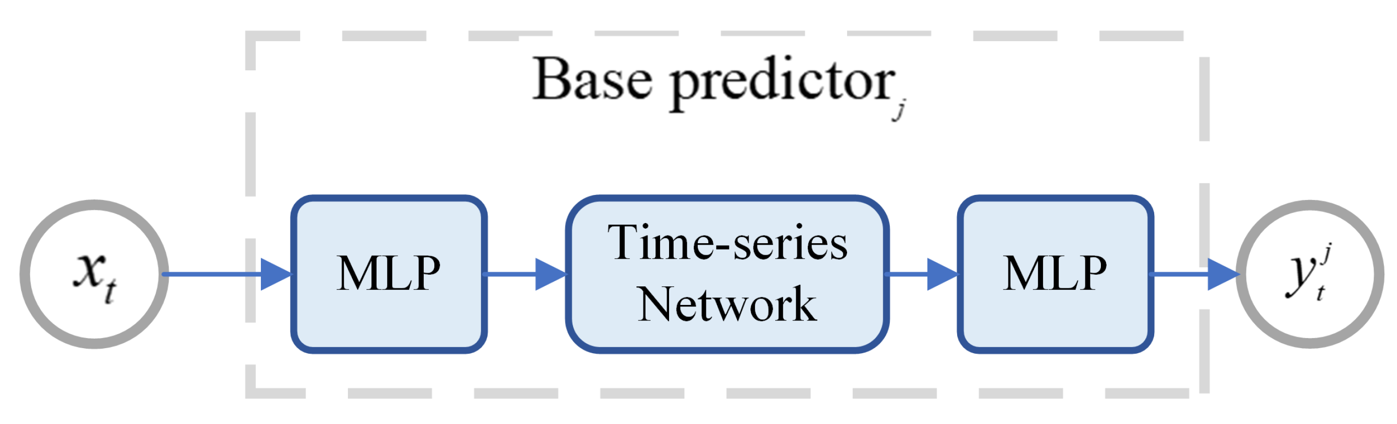
3.3. Base Model Prediction Module

This paper employs n different deep-learning-based base predictors to construct the base model prediction module (BMPM). The fundamental architecture of each base predictor is illustrated in Figure 2, and it includes a common structure comprising a multilayer perceptron (MLP) input layer for feature extraction, a time-series network layer, and an MLP output layer.

Time-series networks are specialized neural network architectures designed to handle time-series data. Time-series data consists of a sequence of data points arranged in chronological order, such as stock prices, sensor readings, or any data with a temporal dimension. Time-series networks are specifically designed to capture time dependencies and patterns within such data. We utilize three types of time-series networks: GRU, ALSTM, and Transformer. Furthermore, different loss functions have varying impacts on the optimization goals of model training, and the choice of the number of hidden layers alters the complexity of the neural network, affecting both the model’s capabilities and style.

Therefore, by using different types of time-series networks, loss functions, and numbers of hidden layers, base predictors of different prediction styles are constructed to achieve more accurate and stable predictions.

The input of the BMPM is the market data $x_t\in R^{m\times k}$ of m stocks, and the outputs are the predictions $y_t\in R^{m\times n}$ of the future returns of the m stocks by each of the n base predictors, as well as the historical losses of the individual base predictors $l_t\in R^{m\times n}$.

The BMPM consists of n base predictors, each of which outputs a corresponding prediction, given by the following equation:

$$y_t^j=predicto{r}_j\left(x_t\right),$$

(1)

$$y_t=\left(y_t^1,y_t^2,\dots ,y_t^n\right).$$

(2)

where $j=\{1,\dots ,n\}$.

The prediction of the base predictor at time t is passed into the corresponding loss function:

$$l_t^j=loss\left(y_t^j\right),$$

(3)

$$l_t=\left(l_t^1,l_t^2,\dots ,l_t^n\right),$$

(4)

DRL-DEM first pre-trains the base predictors using historical market data during the complete training process. In this pre-training process, the base predictors of the same network structure use different loss functions. On one hand, different loss functions have varying impacts on the optimization goals of model training, and they are employed to train base predictors with different prediction styles. On the other hand, each base predictor can retain its historical training error for subsequent input using the corresponding loss function.

3.4. Deep-Reinforcement-Learning-Based Ensemble Module

In order to better adapt to the complex and ever-changing stock market environment, this section optimizes the investment strategy by introducing real-time market feedback as effective supervisory information during the construction of the deep-reinforcement-learning algorithm.

3.4.1. Agent of DRL-DEM

In deep reinforcement learning, the agent is responsible for interacting with the environment. The agent generates action strategies through the actor, and the critic evaluates the quality of the strategies. The agent improves its strategy based on the critic’s feedback and rewards to maximize long-term rewards.

The actor is the key component responsible for strategy generation and action selection in deep reinforcement learning. By continuously learning and improving strategies, the agent can maximize its long-term rewards in complex environments. Figure 3 illustrates the specific implementation of the actor. To enhance the actor’s representational capacity and the independence of policy learning, three MLPs are employed. Each MLP is composed of three linear layers and two $RELU$ function layers. The initial two MLPs receive inputs $y_t$ and $l_t$, respectively. The final MLP combines the outputs from the initial two MLPs. The actor’s final output is computed by applying the $Softmax$ function to the final MLP’s output, and it undergoes additional adjustments in accordance with the temperature coefficient $\sigma$. $\sigma$ controls the degree of exploration of action selection in the actor. By adjusting the value of $\sigma$, a balanced selection of model exploration and utilization can be achieved:

$$A_{1,t}\left(y_t\right)=MLP\left(y_t\right),A_{1,t}\left(l_t\right)=MLP\left(l_t\right),$$

(5)

$$A_{2,t}=MLP(A_{1,t}\left(y_t\right)+A_{1,t}\left(l_t\right)),$$

(6)

$$a_t=Softmax(A_{2,t}/\sigma ),$$

(7)

where $a_t=\left(a_t^1,\dots a_t^i,\dots ,a_t^m\right)$, $a_t^i=\left({\omega }_t^{i1},\dots ,{\omega }_t^{ij},\dots .,{\omega }_t^{in}\right)$ represents the assigned weight of the ith stock corresponding to each of the n base predictors, $i=1,\dots ,m$; ${\omega }_t^{ij}$ represents the weight of the jth base predictor corresponding to the ith stock, $j=1,\dots ,n$. The sum of the weights of the individual base predictors for any stock at any point in time is 1, ${\displaystyle \sum _{j=1}^n}{\omega }_t^{ij}=1,i=1,\dots ,m$.

After selecting the action $a_t$ based on the state $s_t$, the actor network passes both $a_t$ and $s_t$ as inputs to the critic network. The critic network computes an estimate of the action-value function $Q(s_t,a_t)$ based on these inputs and feeds it back to the actor network, which adjusts its policy based on $Q(s_t,a_t)$:

$$Q(s_t,a_t)=E[r(s_t,a_t)+\gamma Q(s_{t+1},\mu \left(s_t\right))].$$

(8)

3.4.2. Calculation Method of Ensemble Prediction

We calculate the ensemble prediction value based on the weight assignment $a_t$ and the prediction result $y_t$ for each base predictor.

At moment t, the prediction value of the base predictors are $y_t=\left(y_t^1,\dots ,y_t^i,\dots ,y_t^m\right)$:

$$y_t^i=\left(b_t^{i1},\dots ,b_t^{in}\right),$$

(9)

where $y_t^i$ is the prediction result of the base prediction model for the ith stock at moment t.

At moment t, the output of the deep-reinforcement-based learning ensemble module is the weight assignment of m stocks corresponding to n base predictors $a_t=\left(a_t^1,\dots ,a_t^i,\dots ,a_t^m\right)$, where $a_t^i=\left({\omega }_t^{i1},\dots ,{\omega }_t^{in}\right)$.

The formula for integrating the prediction is as follows:

$${\stackrel{⏜}{y}}_t=\left[a_t\odot {\left(y_t\right)}^T\right]·e_m=\left({\stackrel{⏜}{y}}_t^1,\dots ,{\stackrel{⏜}{y}}_t^i,\dots ,{\stackrel{⏜}{y}}_t^m\right),$$

(10)

$${\stackrel{⏜}{y}}_t^i=\left(a_t^i\right){\left(y_t^i\right)}^T=({\omega }_t^{i1},\dots ,{\omega }_t^{in}){\left(b_t^{i1},\dots ,b_t^{in}\right)}^T=\sum _{j=1}^n{\omega }_t^{ij}{b}_t^{ij},$$

(11)

where ⊙ represents the Hadamard product, and $e_m$ is all-one vector.

3.4.3. Hybrid Reward Function for DRL-DEM

Deep reinforcement learning trains agents to automatically search for the optimal behavior strategy to maximize their cumulative rewards. The setting of reward function directly determines the learning goal and optimization the direction of the agent. Based on the complexity of the stock market, DRL-DEM uses a hybrid reward function $r_t$ to better guide investment decisions by introducing real-time market feedback as effective supervision information. The $r_t$ consists of three parts: quantitative trading reward, ensemble prediction accuracy reward and ensemble model ranking reward, and formula $r_t$ is defined as follows:

$$r_t=r_t^{profit}+\alpha r_t^{precision}+\beta r_t^{rank},$$

(12)

where $\alpha$ and $\beta$ are hyperparameters balancing the quantitative trading reward, the ensemble prediction accuracy reward, and the ensemble model ranking reward.

Quantifying trading reward $r_t^{profit}$, $r_t^{profit}$ measures the effect of trading with the ensemble prediction model and reflects the practical application value of the ensemble model in the real market environment; $r_t^{profit}$ is defined as follows:

$$r_t^{profit}=\frac{G_t-G_{min}}{G_{max}-G_{min}},$$

(13)

$$G_t=\frac{v_t-v_{t-1}}{v_t},$$

(14)

where $v_t$ is the total capital held at time t.

Ensemble prediction accuracy reward $r_t^{precision}$, $r_t^{precision}$ directly quantifies the error between the ensemble model’s prediction and the true target value, which serves as positive feedback to motivate the model to continuously learn and improve its prediction accuracy; $r_t^{precision}$ is defined as follows:

$$r_t^{precision}=\frac{1}{2}\left(1-\frac{\tau \left({\delta }_t\right)}{n}\right),$$

(15)

where ${\delta }_t$ represents the SMAPE of the ensemble model at time t and $\tau \left({\delta }_t\right)=\{0,\dots ,n\}$ is the quantile of ${\delta }_t$.

Ensemble model ranking reward $r_t^{rank}$. The ranking reward mechanism encourages the ensemble model to leverage its strengths in model combination, thereby enhancing the overall predictive performance. The formula $r_t^{rank}$ is defined as follows:

$$r_t^{rank}=1-\frac{1}{m}\sum _{i=1}^m\frac{{\varsigma }_t^i}{n},$$

(16)

where ${\varsigma }_t^i=\left\{0,1,\dots ,n\right\}$ is the ranking of the performance of the ensemble model in the ith stock at time t among the n base predictors.

In the pre-training process of deep reinforcement learning, the reward function is defined as ${r_t}^{\prime }=\alpha r_t^{precision}+\beta r_t^{rank}$, and in the formal training stage of actual quantitative trading, the reward function will be further extended to (12).

3.4.4. Quantitative Trading Investment Strategy

This section uses a stock ranking strategy to prioritize stocks with higher predicted profit potential for investment. Furthermore, we calculate the quantitative trading reward component of the hybrid reward function using real-time investment returns, as described in Formula (13). DRL-DEM dynamically fine-tunes the base predictor weight configuration based on feedback from the hybrid reward function, aiming to achieve the optimal ensemble prediction result and maximize the return on investment.

At time t, according to the ensemble prediction ${\stackrel{⏜}{y}}_t$ of m stocks, the trading stocks are selected and the allocated funds of the selected stocks are determined. In order to ensure the rationality of the allocated funds, the ensemble prediction value of each stock is transformed as follows to ensure non-negativity:

$${\tilde{y}}_t^i={\stackrel{⏜}{y}}_t^i-min\left({\stackrel{⏜}{y}}_t\right),$$

(17)

$${\stackrel{⏜}{y}}_t=\left({\tilde{y}}_t^1,\dots ,{\tilde{y}}_t^m\right),$$

(18)

where $i=1,\dots ,m$, by sorting ${\stackrel{⏜}{y}}_t$ selects the top q stocks, and the weight of funds allocated to them is:

$$g_t=\left(g_t^1,\dots ,g_t^i,\dots ,g_t^q\right),$$

(19)

$$g_t^i=\frac{{\tilde{y}}_t^i}{{\displaystyle \sum _{j=1}^q}{\tilde{y}}_t^j}.$$

(20)

The funds allocated to the selected stocks are:

$$o_t=\left(o_t^1,\dots ,o_t^i,\dots ,o_t^q\right),$$

(21)

$$o_t^i=c_0·g_t^i,$$

(22)

where $i=1,\dots ,q$ and $c_0$ is the initial investment amount.

3.5. DRL-DEM Objective Function and Algorithm Flow

The agent’s action $a_t$ at each time is determined by a deterministic strategy $\mu$, i.e., $a_t=\mu \left(s_t\right)$.

The actor network is implemented by optimizing the parameters ${\theta }^{\mu }$ of the policy network to maximize the expectation of action selection in different states. The performance of strategy $\mu$ is measured using the function J, which is defined as

$$J=E\left(Q(s,a)\right|s=s_t,a=\mu \left(s_t\right)).$$

(23)

The parameters of the actor network are updated using the Stochastic Gradient Ascent (SGA) method:

$${\nabla }_{{\theta }^{\mu }}J\approx \frac{1}{N}\sum _i{\nabla }_{a}Q\left(s,a|{\theta }^Q\right){|}_{s_i,\mu \left(s_i\right)}{\nabla }_{{\theta }^{\mu }}\mu \left(s|{\theta }^{\mu }\right){|}_{s_i}.$$

(24)

The objective function of the actor is defined as

$$L_a=-E\left(Q(s,a)\right|s=s_t,a=\mu \left(s_t\right)).$$

(25)

The objective function of the critic is defined as

$$L_c=\frac{1}{N}\sum _i{\left(y_i-Q\left(s_i,a_i|{\theta }^Q\right)\right)}^2,$$

(26)

$$y_i=r_i+\gamma Q^{\prime }\left(s_{i+1},{\mu }^{\prime }\left(s_{i+1}|{\theta }^{{\mu }^{\prime }}\right)|{\theta }^{Q^{\prime }}\right),$$

(27)

where $r_i=r_i^{profit}+\alpha r_i^{precision}+\beta r_i^{rank}$.

Combining the above categories, the total objective function of DRL-DEM is defined as

$$L=L_a+L_c.$$

(28)

The total objective function (28) combines the actor and critic objective functions, but when updating the actor and critic networks, they are updated separately based on (24) and (26).

In the training process based on the Deep Deterministic Policy Gradients (DDPG) algorithm, to enhance training stability, both the actor network and the critic network consist of both a target network and a real network. The target networks within the actor and critic networks help address the exploration–exploitation problem. The real networks update the parameters of the target networks through a soft update, and the formula is as follows:

$$\left\{\begin{array}{c}{\theta }^{{\mu }^{\prime }}\leftarrow \tau {\theta }^{\mu }+\left(1-\tau \right){\theta }^{{\mu }^{\prime }}\\ {\theta }^{Q^{\prime }}\leftarrow \tau {\theta }^Q+\left(1-\tau \right){\theta }^{Q^{\prime }}\end{array}\right.$$

(29)

where ${\theta }^{\mu }$ and ${\theta }^Q$ are the parameters of the real actor network and the real critic network, respectively. ${\theta }^{{\mu }^{\prime }}$ and ${\theta }^{Q^{\prime }}$ are the parameters of the target actor network and the target critic network, respectively, and $\tau$ is the moving average coefficient.

The training process in this article is divided into two stages. In the first stage, we first pre-train each base predictor using historical market data. This pre-training strategy not only ensures better performance of the base predictor in the initial stage, but also provides a basis for the subsequent second-stage training process. In the second stage, an alternating iterative algorithm is employed to simultaneously train the base predictors and the deep-reinforcement-learning model. Specifically, in the process of deep-reinforcement-learning training, after each round of parameter updates for the actor and critic networks, the base predictors employ the smooth L1 loss function and iteratively updates its parameters through gradient descent to enhance performance. The detailed process is shown in Algorithm 1.

Algorithm 1 DRL-DEM Algorithm Flow

Initialize base predictor network parameters $\phi$, critic network parameters ${\theta }^Q$, actor network parameters ${\theta }^{\mu }$ and experience playback replay buffer for  $i=1,2,\dots ,n$  do     pre-trained base predictor networks     input $x_t$, output $y_t$ and $l_t$ end for copy ${\theta }^Q$, ${\theta }^{\mu }$ to ${\theta }^{Q^{\prime }}$, ${\theta }^{{\mu }^{\prime }}$ via (29) input $y_t$, $l_t$ pre-trained actor networks for  $episode=1,2,\dots ,episodes$  do     for $t=1,\dots ,steps$ do         get action $a_t=\mu \left(s_t\right)$ based on the current strategy         calculate ${\stackrel{⏜}{y}}_t$ according to (10)         calculate $r_t^{profit}$ according to (13)         execute action $a_t$ to get $s_{t+1}$         calculate $r_t^{precision}$ according to (15)         calculate $r_t^{rank}$ according to (16)         calculate the total return $r_t$ according to (12)         store $\left(s_t,a_t,r_t,s_{t+1}\right)$ in the replay buffer     end for     if t mod D then         sample mini-batch conversion sequences from the replay buffer         update actor network parameters ${\theta }^{\mu }$ by (24)         update critic network parameters ${\theta }^Q$ by (26)         update base predictor network parameters $\phi$     end if end for

4. Experimental Results and Analysis

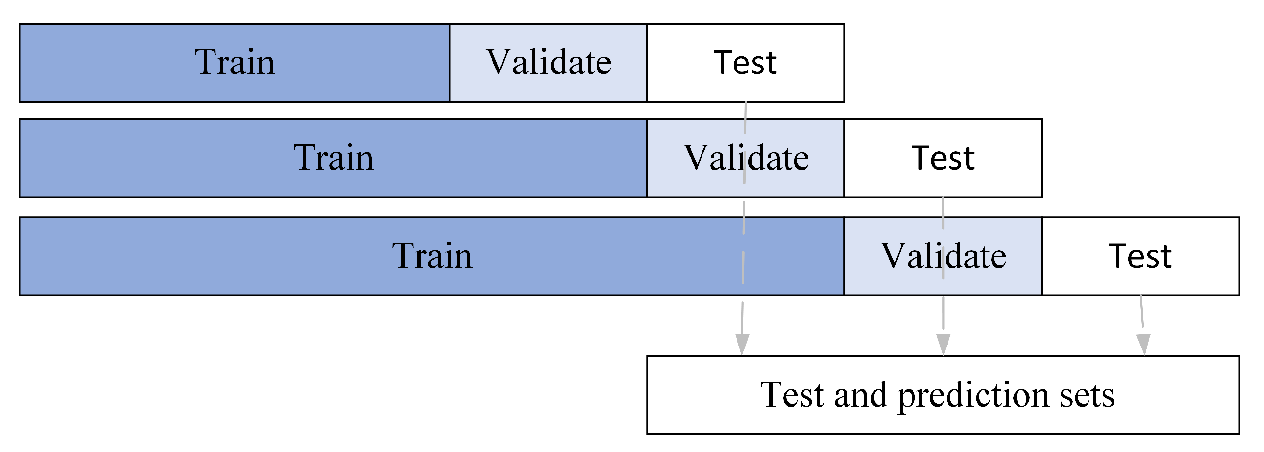
The experimental evaluation approach presented in this paper thoroughly considers both the accuracy of prediction and the performance in investment. It assesses the predictive capability of the employed model by employing statistical metrics such as mean square error and symmetrical average percentage error. Moreover, it incorporates key stock risk–return indicators, such as the Sharpe ratio, cumulative return, annualized rate of return, and maximum retracement, to evaluate its tangible impact on investment outcomes.

4.1. Dataset

Our experiments are conducted using two datasets: the SSE 50 dataset obtained from Baostock (www.baostock.com), covering the time period from 18 October 2011 to 31 March 2023, and the NASDAQ 100 dataset obtained from Yahoo Finance (https://finance.yahoo.com), spanning from 2 August 2010 to 31 March 2023. We excluded stocks that were incomplete or delisted throughout the period, ultimately retaining 38 and 78 constituents, respectively. We selected the main technical indicators affecting stock price fluctuations as the characterization factors of stock data, including opening price, closing price, high price, low price, trading volume, and trading turnover.

To enhance the learning capabilities of DRL-DEM and facilitate the discovery of sequential patterns within stock data, we adopted a rolling training, validation, and testing approach, as illustrated in Figure 4 and elaborated upon in

Table 2. Information on the SSE50 dataset.

Dataset	Training Set		Validation Set		Test Set
SSE 50	Period	Sample Size	Period	Sample Size	Period	Sample Size
1	2011/10/18–2019/12/27	1997	2019/12/30–2020/10/29	200	2020/10/30–2021/8/20	200
2	2011/10/18–2020/10/29	2197	2020/10/30–2021/8/20	200	2021/8/23–2022/6/23	200
3	2011/10/18–2021/8/20	2397	2021/8/23–2022/6/23	200	2022/6/24–2023/3/31	189

and

Table 3. Information on the NASDAQ 100 dataset.

Dataset	Training Set		Validation Set		Test Set
NASDAQ 100	Period	Sample Size	Period	Sample Size	Period	Sample Size
1	2010/8/2–2020/2/11	2399	2020/2/12–2020/11/24	200	2020/11/25–2021/9/13	200
2	2010/8/2–2020/11/24	2599	2020/11/25–2021/9/13	200	2021/9/14–2022/6/29	200
3	2010/8/2–2021/9/13	2799	2021/9/14–2022/6/29	200	2022/6/30–2023/3/31	190

. These tables provide comprehensive statistical information concerning the division intervals.

4.2. Experimental Settings

4.2.1. Base Predictor Settings

This experiment utilizes three representative time-series networks: GRU, ALSTM, and Transformer, in order to construct a diverse set of base predictors. Within each category of time-series network, we have developed two relatively independent models by adjusting various parameter settings. This leads to the creation of a total of six unique base predictors for our study:

• Base Predictor 1: GRU time-series network with 64 hidden units, trained using Mean Squared Error Loss.
• Base Predictor 2: GRU time-series network with 128 hidden units, trained using Smooth L1 Loss.
• Base Predictor 3: ALSTM time-series network with 64 hidden units, trained using Mean Squared Error Loss.
• Base Predictor 4: ALSTM time-series network with 128 hidden units, trained using Smooth L1 Loss.
• Base Predictor 5: Transformer time-series network with 64 hidden units, trained using Mean Squared Error Loss.
• Base Predictor 6: Transformer time-series network with 128 hidden units, trained using Smooth L1 Loss.

These six base predictors differ in their ability to capture short- and long-term dependencies, sensitivity to outliers, and data noise by employing different neural network architectures and loss functions. These differences allow them to adapt to a variety of data characteristics, providing diversity and flexibility in predictive capabilities. By integrating these base predictors, more stable predictions can be achieved, taking full advantage of their respective strengths.

4.2.2. Hyperparameter Settings

We determined the optimal parameter for T through a grid search method, where the value range for T was chosen from $\{5,10,15,20,25,30\}$. Ultimately, the optimal time-series window size was found to be T = 15. Additionally, we set the discount factor $\gamma$ to 0.99, both components $\alpha$ and $\beta$ in the hybrid reward function were set to 1, and the learning rate for deep reinforcement learning was established at $1\times {10}^{-5}$. The initial investment fund was set at 10,000,000, and the transaction fee rate was configured as 0.15%.

4.2.3. Investment Strategy Settings

We set a trading cycle of d days, buy stocks on t days, sell stocks on $t+d$ days in preparation for the next buying phase. We start buying stocks at time t:

$$h_t=⌊\frac{o_t}{p_t}⌋,$$

(30)

$$c_t=c_0-p_t{h}_t^T-cos{t}_t,$$

(31)

where $h_t$ is the stock position vector at time t, $h_t$ is the stock price vector at time t, $o_t$ is the stock investment fund vector at time t, $c_t$ is the cash at time t and $cos{t}_t$ represents the transaction cost deducted from each transaction, in order to prevent the cash held from being negative, resulting in behavior that is inconsistent with market logic. To ensure compliance with real logic, the fund non-negative constraint formula is as follows:

$$c_t=c_0-p_t{h}_t^T-cos{t}_t⩾0.$$

(32)

During the period from time t to $t+d-1$, we maintain the position unchanged.

At the end of the holding period at time $t+d$, the trader sells the holdings to obtain the current cash:

$$c_{t+d}=c_t+p_{t+d}{h}_{t+d}^T.$$

(33)

By defining the cash $c_t$ held at time t, the number of stock positions $h_t$, and the stock price vector $p_t$, we can calculate the total asset value $v_t$ as follows:

$$v_t=c_t+p_t{h}_t^T.$$

(34)

The rate of return for each time step is $G_t=\frac{v_t - v_{t-1}}{v_t}$.

4.3. Evaluation Indicators

4.3.1. Prediction Accuracy Evaluation Component

We selected two metrics, mean square error and symmetric mean absolute percentage error, to evaluate the prediction performance of DRL-DEM.

• Mean Square Error (MSE): measures the average error of the model. The smaller the value, the smaller the error between the model’s prediction and the actual observed value, and the better the model performance.

  $$MSE=\frac{1}{n}\sum _{i=1}^n{\left({\stackrel{⏜}{y}}_i-y_i\right)}^2,$$

  (35)

  where ${\stackrel{⏜}{y}}_i$ is the predicted value and $y_i$ is the true value.
• Symmetric Mean Absolute Percentage Error (SMAPE): measures the percentage error of the model. The smaller the value, the better the model performance.

  $$SMAPE=\frac{100\%}{n}\sum _{i=1}^n\frac{\left|{\stackrel{⏜}{y}}_i-y_i\right|}{\left(\left|{\stackrel{⏜}{y}}_i\right|+\left|y_i\right|\right)/2},$$

  (36)

  where ${\stackrel{⏜}{y}}_i$ is the predicted value and $y_i$ is the true value.

4.3.2. Portfolio Return Evaluation Component

In order to evaluate the profitability of the DRL-DEM, we selected four indicators: cumulative return, Sharpe ratio, annualized rate of return, and maximum drawdown.

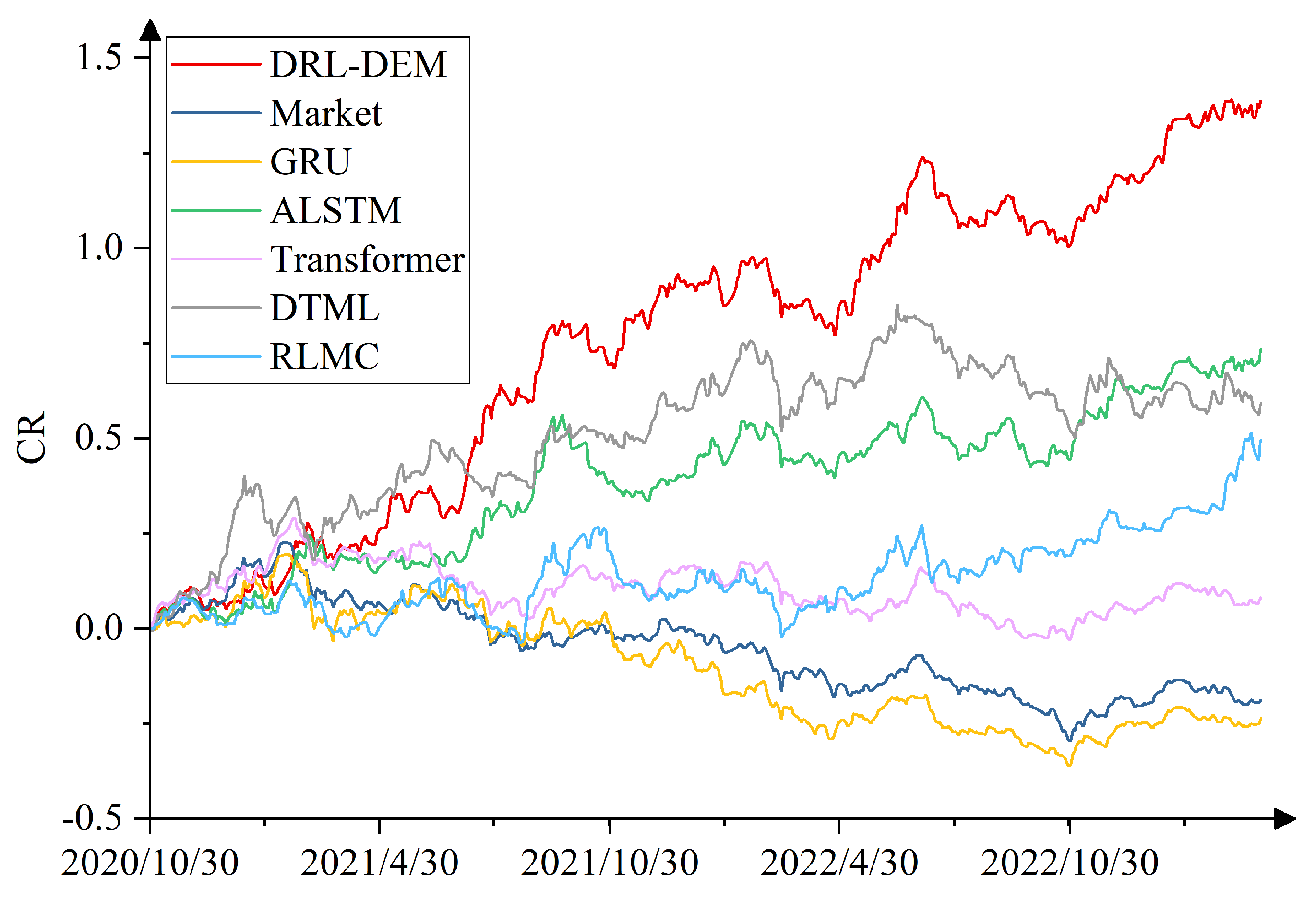
• Cumulative Return (CR): represents the total return from the initial investment to the end. The larger the value, the better the model performance.

  $$CR=\frac{v_t-v_0}{v_0},$$

  (37)

  where $v_t$ is the total assets at time t, $v_0$ is the initial assets.
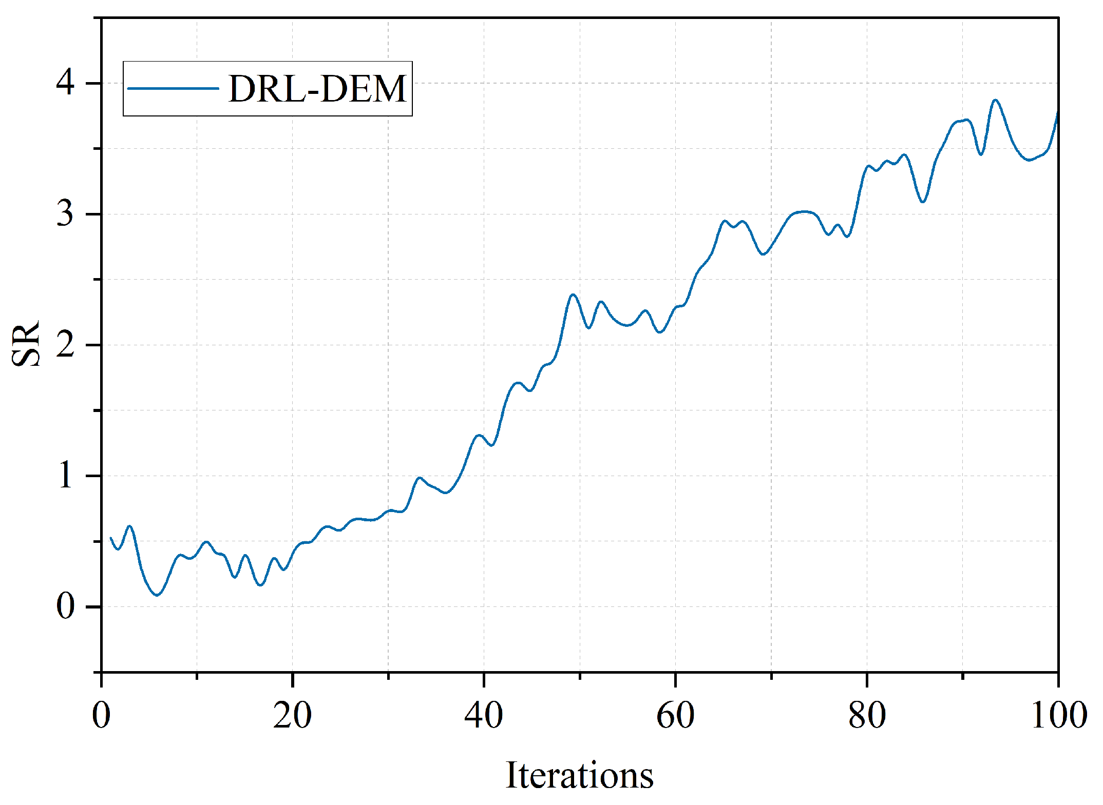
• Sharpe Ratio (SR): SR is used to evaluate the profitability and risk tolerance of the model. The larger the value, the better the model performance.

  $$SR=\frac{E\left[RO{R}_p\right]-r_f}{{\sigma }_p},$$

  (38)

  where $E\left[RO{R}_p\right]$ is the expectation of portfolio return, $r_f$ is the risk-free interest rate, and ${\sigma }_p$ is the standard deviation of portfolio return.
• Annualized Rate of Return (ARR): represents the average return of the investment portfolio within one year. The larger the value, the better the model performance.

  $$ARR={(1+CR)}^{\frac{252}{e}}-1,$$

  (39)

  where e represents the transaction duration, 252 represents the number of trading days in a year.
• Maximum Drawdown (MDD): represents the maximum short-term loss suffered during the entire investment process. The smaller the value, the better the model performance.

  $$MDD=\underset{i\in \left(0,t\right)}{max}\left\{\underset{j\in \left(0,i\right)}{max}\frac{v_j-v_i}{v_j}\right\},$$

  (40)
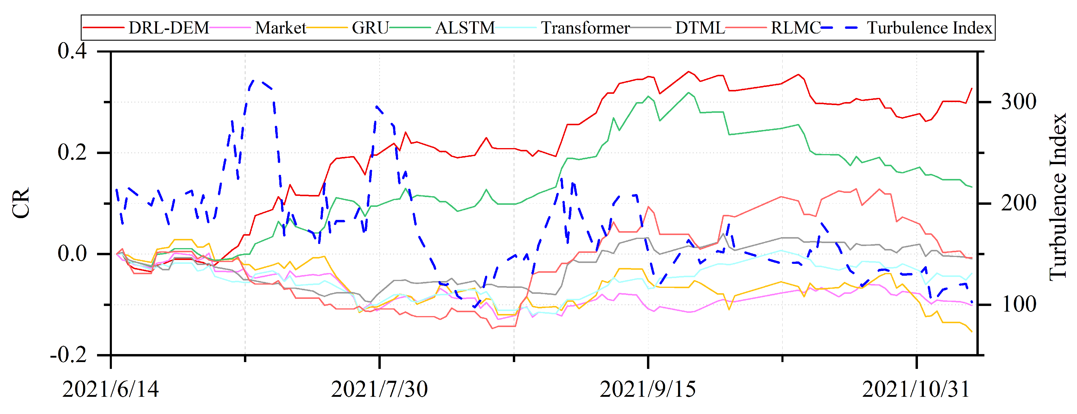
• Turbulence index: measure recent market risk conditions. The index value is usually stable within a certain threshold. If the index suddenly breaks through, it indicates an extreme situation in the market.

  $$TurbulenceIndex=(z_t-\epsilon ){\Sigma }^{-1}{(z_t-\epsilon )}^T,$$

  (41)

  where $z_t$ is the return on assets at the current moment t, $\epsilon$ is the average of historical returns, and $\Sigma$ is the covariance of historical returns.

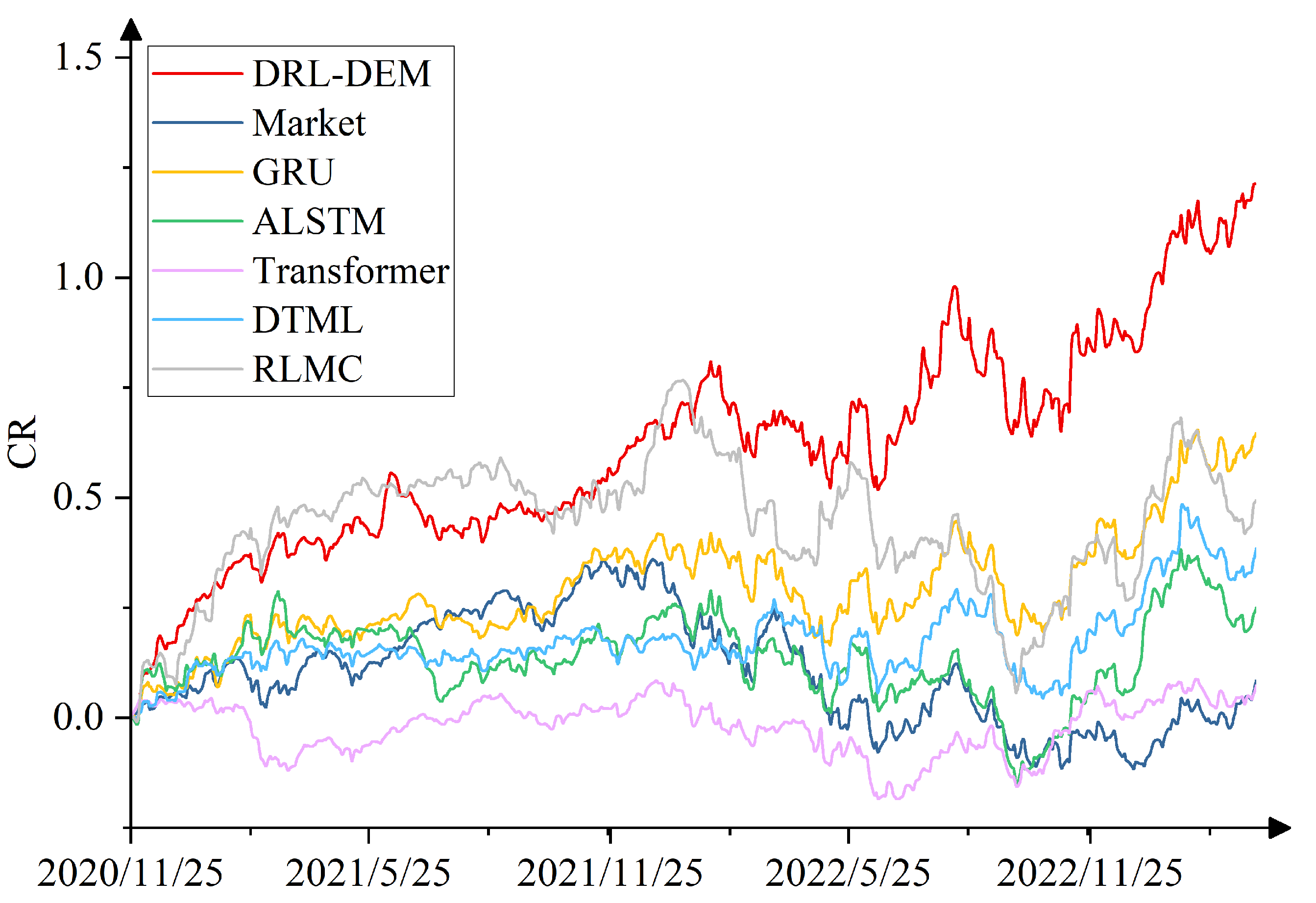
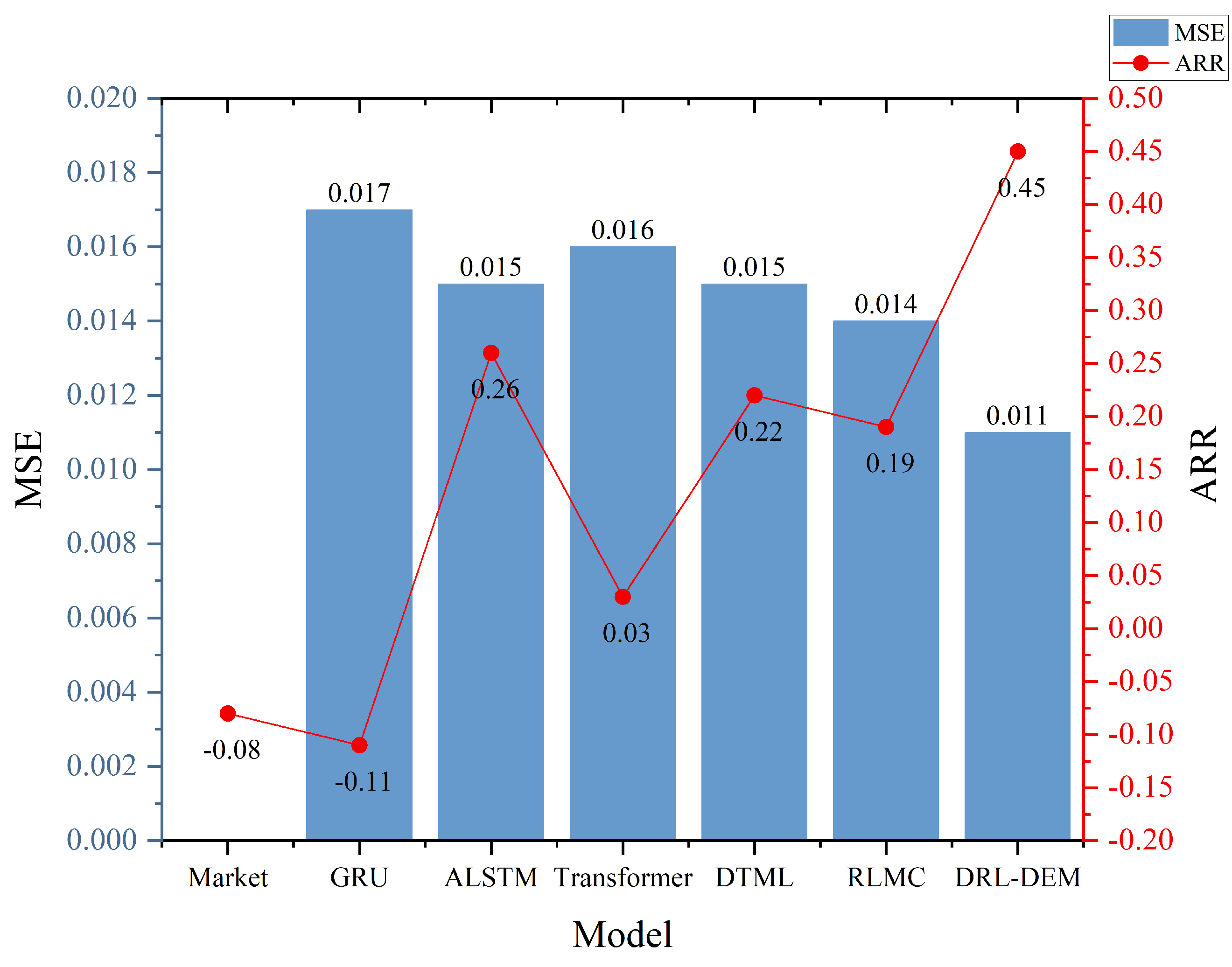
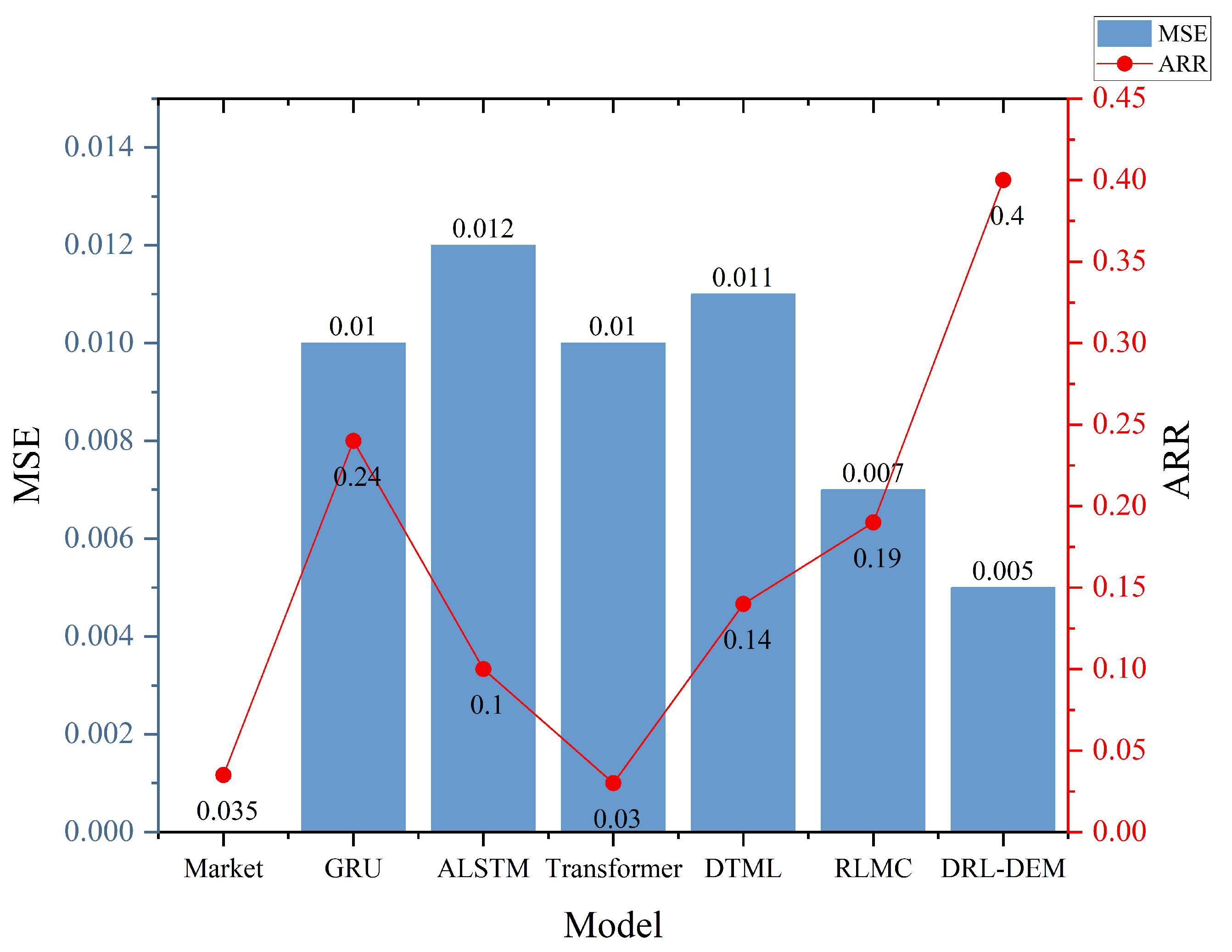
4.4. Comparison Experiment

The following are several comparison models selected for this article. For the rationality of the experiment, this study added the same trading strategy to the comparison model to conduct comparative experiments. All models underwent training and testing on identical datasets, with consistent training and testing distributions.

• Market: A widely adopted benchmark investment strategy that involves buying a broad market index from the first day of the test set and holding it until the last day of the test set, with no active trading decisions. We use the SSE50 index as the market benchmark for the SSE50 dataset, and the NASDAQ 100 index as the market benchmark for the NASDAQ 100 dataset.
• GRU [28]: Controls the flow of information through a gating mechanism and is a simple benchmark widely used in stock prediction.
• ALSTM [10]: Combines LSTM, which is used to capture long- and short-term dependencies of stock data, and the self-attention mechanism, which allows the model to dynamically focus on information at different time steps based on the context.
• Transformer [11]: As a deep learning architecture that processes stock data through self-attention and multi-attention mechanisms, as well as positional coding.
• DTML [30]: Extracting stock contexts through attention mechanism, fusing the overall market trend to generate multi-level contexts, and utilizing Transformer to learn dynamic asymmetric correlations among stocks.
• RLMC [20]: Training an agent to automate the optimal selection and combination of multiple predictive models through deep reinforcement learning.

The performance of various models on two datasets, the SSE 50 and NASDAQ 100, is demonstrated in Figure 5 and Figure 6. Notably, the CR (1.38, 1.21) curve of DRL-DEM outperforms the curves of all comparative models. Furthermore, as shown in Figure 7 and Figure 8, different models’ MSE and ARR indicators are presented, and it is evident that DRL-DEM achieves the best performance in both datasets. Additionally, as highlighted in

Table 4. Comparison of evaluation indices of different models.

Model	SSE 50						NASDAQ 100
	SR	MDD	CR	ARR	MSE	SMAPE	SR	MDD	CR	ARR	MSE	SMAPE
Market	−0.60	0.43	−0.19	−0.08			0.02	0.36	0.08	0.035
GRU	−0.61	0.46	−0.23	−0.11	0.017	9.60	0.84	0.19	0.64	0.24	0.010	8.48
ALSTM	1.21	0.14	0.73	0.26	0.015	9.09	0.26	0.35	0.25	0.10	0.012	8.89
Transformer	0.02	0.25	0.08	0.03	0.016	8.99	0.003	0.25	0.07	0.03	0.010	8.49
DTML	0.85	0.20	0.59	0.22	0.015	9.07	0.55	0.20	0.38	0.14	0.011	8.68
RLMC	0.68	0.23	0.49	0.19	0.014	8.99	0.59	0.40	0.49	0.19	0.007	6.94
DRL-DEM	2.20	0.11	1.38	0.45	0.011	7.41	1.53	0.17	1.21	0.40	0.005	6.19

Bold fonts in the table indicate the best results in each indicator.

, when evaluating the performance metrics of these models, DRL-DEM achieves the lowest MSE values of 0.011 and 0.005, as well as the smallest SMAPE values of 7.41 and 6.19. Additionally, it attains the highest SR values of 2.20 and 1.53 and the highest ARR values of 0.45 and 0.40.

In contrast to single-stock prediction trading models like GRU, ALSTM, and Transformer, DRL-DEM demonstrates improvements in both prediction accuracy and investment returns. Moreover, across different datasets, while GRU, ALSTM, and Transformer exhibit fluctuating return performances, DRL-DEM effectively adapts to the volatile stock market environment. Compared to RLMC, DRL-DEM shows a significant reduction in MSE by 21.4% and 28.6%, along with an impressive increase in SR by 224% and 159%, and a substantial improvement in CR by 182% and 147% in the SSE 50 and NASDAQ 100 datasets, respectively. DRL-DEM also outperforms DTML in terms of achieving higher SR and CR. Moreover, DRL-DEM consistently demonstrates strong performance across all other evaluation metrics in both datasets.

The experimental results underscore that DRL-DEM achieves superior prediction accuracy and excels in pursuing returns while mitigating risks. This achievement can be attributed to several key features, including the utilization of a deep-reinforcement-learning ensemble method, the incorporation of real-time market feedback as an additional signal for the algorithm, and the implementation of a global co-optimization model.

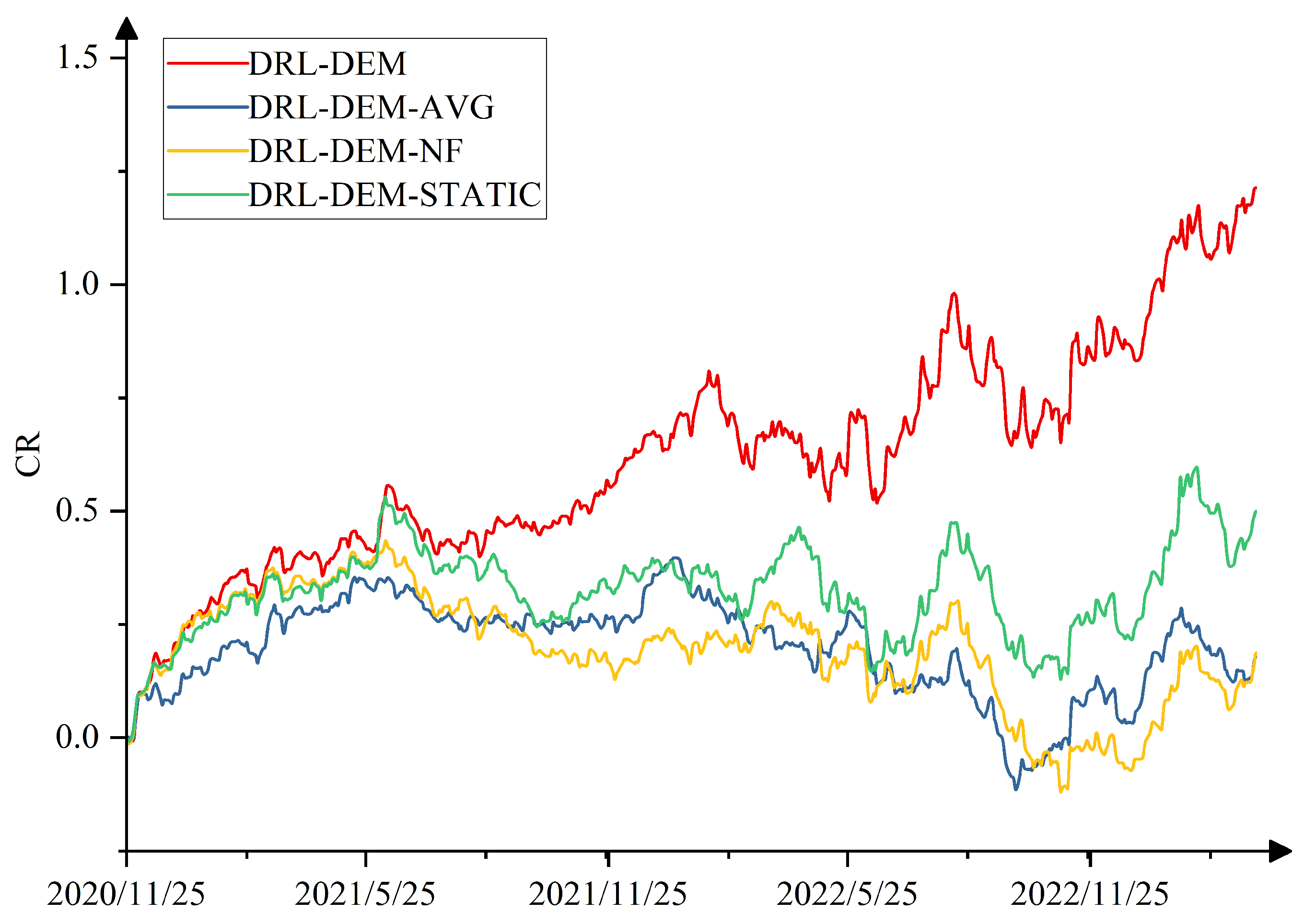
4.5. Ablation Experiment

To assess the effectiveness of the weight allocation method based on deep reinforcement learning, real-time market feedback, and global collaborative optimization within DRL-DEM, we conducted ablation experiments on two datasets. These ablation experiments for DRL-DEM were labeled as follows:

• DRL-DEM-AVG: Without adopting the weight allocation method based on deep reinforcement learning, weights are evenly distributed among individual base predictors.
• DRL-DEM-NF: Without introducing real-time market feedback, only two components of the mixed reward function, namely ensemble prediction accuracy reward and ensemble prediction model ranking reward, are retained.
• DRL-DEM-STATIC: Without employing the global collaborative optimization approach, base predictors are no longer updated during the training process.

The results from the ablation experiments conducted on the SSE 50 and NASDAQ 100 datasets are presented in Figure 9 and Figure 10 and

Table 5. Comparison of evaluation indices of DRL-DEM ablation test.

Model	SSE 50						NASDAQ 100
	SR	MDD	CR	ARR	MSE	SMAPE	SR	MDD	CR	ARR	MSE	SMAPE
DRL-DEM-AVG	−0.04	0.22	0.05	0.02	0.015	9.03	0.22	0.37	0.19	0.08	0.010	8.30
DRL-DEM-NF	0.76	0.20	0.44	0.17	0.011	7.53	0.19	0.39	0.18	0.07	0.006	6.20
DRL-DEM-STATIC	0.37	0.18	0.25	0.10	0.013	8.49	0.66	0.27	0.50	0.19	0.007	7.90
DRL-DEM	2.20	0.11	1.38	0.45	0.011	7.41	1.53	0.17	1.21	0.40	0.005	6.19

Bold fonts in the table indicate the best results in each indicator.

. These results clearly demonstrate that DRL-DEM outperforms DRL-DEM-AVG, DRL-DEM-NF, and DRL-DEM-STATIC across various metrics. Specifically, the SR values achieved by DRL-DEM are 2.20 and 1.53, superior to the other methods. At the same time, DRL-DEM obtains CR values of 1.38 and 1.21, along with ARR values of 0.45 and 0.40, again surpassing the other techniques. Furthermore, DRL-DEM achieves higher prediction accuracy, evidenced by lower MSE values of 0.011 and 0.005 as well as smaller SMAPE values of 7.41 and 6.19. Compared with DRL-DEM-AVG, the excellent performance of DRL-DEM fully proves the effectiveness of the weight optimization method based on deep reinforcement learning. In addition, the improvement in CR index of DRL-DEM compared to DRL-DEM-NF also highlights the key role of introducing real-time market feedback to improve the investment effect of the model. Finally, the comparison with DRL-DEM-STATI further emphasizes the importance of adopting a global collaborative optimization approach. The superior performance of DRL-DEM demonstrates that this method can effectively ensemble various base predictors to achieve more accurate predictions and achieve better performance in quantitative trading.

4.6. Parametric Analysis

4.6.1. Base Predictor Volume Analysis

In order to analyze the impact of the number of base predictors on the ensemble model’s performance, a series of experiments were conducted using varying numbers of base predictors, ranging from 3 to 8. In addition to the six base predictors used in this article, base predictor 7 is constructed using a GRU time-series network with 32 hidden units, trained using Mean Squared Error Loss. Base predictor 8 is constructed using an ALSTM time-series network with 32 hidden units, trained using Mean Squared Error Loss.

Table 6. Base predictor volume analysis.

Number of Base Predictors	Selected Base Predictors	MSE	SMAPE
3	1, 3 and 5	0.0149	8.96
4	1, 2, 3 and 5	0.0135	8.02
5	1, 2, 3, 4 and 5	0.0127	7.97
6	1, 2, 3, 4, 5 and 6	0.0110	7.41
7	1, 2, 3, 4, 5, 6 and 7	0.0133	8.14
8	1, 2, 3, 4, 5, 6, 7 and 8	0.0128	7.72

Bold fonts in the table indicate the best results.

displays the MSE and SMAPE results, where ’Selected Base Predictors’ represent the numerical identifiers of the chosen base predictors. Clearly, as the number of base predictors increases from 3 to 6, there is a consistent decrease in MSE to 0.0110, accompanied by a reduction in SMAPE to 7.41. These trends signify an improvement in prediction accuracy. However, further increasing the number of base predictors to 7 and 8 results in a slight rebound in both MSE and SMAPE.

Experimental results show that after the number of base predictors reaches a certain number, continuing to increase the number of base predictors will not bring further significant improvement in performance. Consequently, this article employs 6 base predictors to construct the BMPM.

4.6.2. Time-Series Step Analysis

To evaluate the prediction stability of DRL-DEM, we conducted a parameter analysis for the time-series window length T. We experimented with various window lengths: 5, 10, 15, 20, 25, and 30 days. The results in Figure 11 reveal that a window length of 5 or 10 days can capture meaningful features. However, longer window lengths exceeding 15 days overly emphasize long-term historical data while neglecting short-term characteristics, leading to increased MSE. As a result, we selected a time-series window length of 15 days in our study.

4.6.3. Hyperparametric Analysis

Furthermore, objective function (28) has three hyperparameters, including the discount factor $\gamma$, as well as $\alpha$ and $\beta$ in the hybrid reward function $r_t$. To assess the impact of three parameters on the model, we explored various value ranges between 0.3 and 1. The experimental results, as depicted in Figure 12, indicate that as the values of three parameters vary, the return curve exhibits a relatively stable trend, with minimal fluctuations within the range of 0.4 to 0.9. Notably, when these parameters are set in the interval of 0.9 to 1, an overall enhancement in model performance becomes evident. The most favorable results were achieved when the discount factor $\gamma$ was set to 0.99, and likewise, when $\alpha$ and $\beta$ were both assigned a value of 1.

4.7. Algorithm Performance Analysis

Due to the complexity and instability of the stock market, deep reinforcement learning tends to face large fluctuations during the training process, making it difficult to reach a converged state. Figure 13 shows the changes in the SR during the DRL-DEM training process. It can be seen that the SR shows a continuous improvement trend during the continuous iteration and optimization process. It shows that the model has the ability to adapt to changes in the stock market, and can effectively respond to market fluctuations, providing investors with stable and reliable predictions and decision-making basis.

4.8. Case Analysis

To assess the effectiveness of DRL-DEM in a complex market environment, we performed case analyses on the SSE 50 and the NASDAQ 100. The initial case analysis scrutinized the market conditions of the SSE50 Index spanning from June to October 2021. As seen in Figure 14, the SSE50 Index followed a downward trajectory from June to October 2021. Notably, there was a significant decline in July and August, with relatively minor fluctuations in other periods. This downturn resulted from a combination of macroeconomic factors, including a slowdown in China’s economic growth, decreased industrial production, and real estate regulations, all of which eroded market confidence. However, the ensemble optimization approach proposed in this study exhibited remarkable adaptability within this challenging market environment, effectively managing risks and delivering improved returns.

The second case analysis was conducted using the market conditions of the NASDAQ 100 Index between June and August 2022. Throughout this period, the Federal Reserve’s interest rate hikes and the market’s fluctuating expectations concerning future rate increases induced market instability. This instability is evident in the elevated levels of turbulence index and heightened risk. Nevertheless, in the face of these turbulent market conditions, as illustrated in Figure 15, our proposed model has consistently demonstrated its capacity to provide reliable forecasts, resulting in substantial returns for investors.

5. Conclusions

This paper introduces the deep-reinforcement-learning-based dynamic ensemble model for stock prediction (DRL-DEM). DRL-DEM leverages deep reinforcement learning to combine multiple deep learning-based stock prediction models. It dynamically adjusts the weights of base predictors, selecting the optimal combination of base predictors to enhance its adaptability to stock market environments. When individual base predictors underperform in specific market environments, the system can automatically reduce their influence. Furthermore, by incorporating real-time investment returns as an additional feedback signal into the deep-reinforcement-learning algorithm. This not only enhances prediction accuracy but also takes into account real investment returns, aligning the model more closely with actual investment requirements. In the training process, both the base predictors and deep-reinforcement-learning components are simultaneously trained using an alternating iterative algorithm. Experimental results demonstrate that DRL-DEM outperforms the comparison model in two datasets: the SSE 50 and the NASDAQ 100. This indicates that DRL-DEM is effective at ensemble learning with base predictors across different market environments. Furthermore, it exhibits a more prominent performance in pursuing benefits and mitigating risks.

Our further work will introduce richer stock features, such as text data extracted from news and social media. DRL-DEM constructed in this article has the potential to incorporate new data sources like text by adding text-based predictors to the ensemble model. Additionally, we will further consider the issue of model time complexity in future research work.

References

1. Nti, I.K.; Adekoya, A.F.; Wevori, B.A. A comprehensive evaluation of ensemble learning for stock-market prediction. J. Big Data 2008, 7, 20. [Google Scholar] [CrossRef]
2. Khashei, M.; Hajirahimi, Z. A comparative study of series ARIMA/MLP hybrid models for stock price forecasting. Commun. Stat. Simul. Comput. 2019, 48, 2625–2640. [Google Scholar] [CrossRef]
3. Pradhan, R.P. Information communications technology (ICT) infrastructure impact on stock market-growth nexus: The panel VAR model. In Proceedings of the 2014 IEEE International Conference on Industrial Engineering and Engineering Management, Selangor, Malaysia, 9–12 December 2014; pp. 607–611. [Google Scholar]
4. Eapen, J.; Verma, A.; Bein, D. Improved big data stock index prediction using deep learning with CNN and GRU. Int. J. Big Data Intell. 2020, 7, 202–210. [Google Scholar] [CrossRef]
5. Swathi, T.; Kasiviswanath, N.; Rao, A.A. An optimal deep learning-based LSTM for stock price prediction using twitter sentiment analysis. Appl. Intell. 2022, 52, 13675–13688. [Google Scholar] [CrossRef]
6. Olorunnimbe, K.; Viktor, H. Deep learning in the stock market—A systematic survey of practice, backtesting, and applications. Artif. Intell. Rev. 2023, 56, 2057–2109. [Google Scholar] [CrossRef] [PubMed]
7. Nelson, D.M.Q.; Pereira, A.C.M.; De Oliveira, R.A. Stock market’s price movement prediction with LSTM neural networks. In Proceedings of the 2017 International Joint Conference on Neural Networks, Anchorage, AK, USA, 14–19 May 2017; pp. 1419–1426. [Google Scholar]
8. Liu, Y.; Liu, X.; Zhang, Y.; Li, S. CEGH: A hybrid model using CEEMD, entropy, GRU, and history attention for intraday stock market forecasting. Entropy 2022, 25, 71. [Google Scholar] [CrossRef] [PubMed]
9. Chen, J.; Du, J.; Xue, Z.; Kou, F. Prediction of financial big data stock trends based on attention mechanism. In Proceedings of the 2020 IEEE International Conference on Knowledge Graph, Nanjing, China, 9–11 August 2020; pp. 152–156. [Google Scholar]
10. Cheng, L.C.; Huang, Y.H.; Wu, M.E. Applied attention-based LSTM neural networks in stock prediction. In Proceedings of the 2018 IEEE International Conference on Big Data, Seattle, WA, USA, 10–13 December 2018; pp. 4716–4718. [Google Scholar]
11. Vaswani, A.; Shazeer, N.; Parmar, N.; Uszkoreit, J.; Jones, L.; Gomez, A.N.; Kaiser, L.; Polosukhin, I. Attention is all you need. Adv. Neural Inf. Process. Syst. 2017, 30, 5998–6008. [Google Scholar]
12. Makridakis, S.; Spiliotis, E.; Assimakopoulos, V. The M4 Competition: Results, findings, conclusion and way forward. Int. J. Forecast. 2018, 34, 802–808. [Google Scholar] [CrossRef]
13. Samal, S.; Dash, R. A novel MCDM ensemble approach of designing an ELM based predictor for stock index price forecasting. Intell. Decis. Technol. 2022, 16, 387–406. [Google Scholar] [CrossRef]
14. Shrivastav, L.K.; Kumar, R. An ensemble of random forest gradient boosting machine and deep learning methods for stock price prediction. J. Inf. Technol. 2022, 15, 1–19. [Google Scholar] [CrossRef]
15. Kuncheva, L.I.; Whitaker, C.J. Measures of diversity in classifier ensembles and their relationship with the ensemble accuracy. Mach. Learn. 2003, 51, 181–207. [Google Scholar] [CrossRef]
16. Mehta, S.; Rana, P.; Singh, S.; Sharma, A.; Agarwal, P. Ensemble learning approach for enhanced stock prediction. In Proceedings of the Twelfth International Conference on Contemporary Computing (IC3), Noida, India, 8–10 August 2019; pp. 1–5. [Google Scholar]
17. Zhao, J.; Takai, A.; Kita, E. Weight-training ensemble model for stock price forecast. In Proceedings of the 2022 IEEE International Conference on Data Mining Workshops, Orlando, FL, USA, 28 November–1 December 2022; pp. 1–6. [Google Scholar]
18. Nti, I.K.; Adekoya, A.F.; Wevori, B.A. Efficient stock-market prediction using ensemble support vector machine. Open Comput. Sci. 2020, 10, 153–163. [Google Scholar] [CrossRef]
19. Sun, M.; Wang, J.; Li, Q.; Zhou, J.; Cui, C.; Jian, M. Stock index time series prediction based on ensemble learning model. J. Comput. Methods Sci. Eng. 2023, 23, 63–74. [Google Scholar] [CrossRef]
20. Fu, Y.; Wu, D.; Boulet, B. Reinforcement learning based dynamic model combination for time series forecasting. In Proceedings of the AAAI Conference on Artificial Intelligence, Vancouver, BC, Canada, 22 February–1 March 2022; pp. 6639–6647. [Google Scholar]
21. Lemke, C.; Gabrys, B. Meta-learning for time series forecasting and forecast combination. Neurocomputing 2010, 73, 2006–2016. [Google Scholar] [CrossRef]
22. Latif, R.M.A.; Naeem, M.R.; Rizwan, O.; Farhan, M. A smart technique to forecast karachi stock market share-values using ARIMA model. In Proceedings of the 2021 International Conference on Frontiers of Information Technology (FIT), Islamabad, Pakistan, 13–14 December 2021; pp. 317–322. [Google Scholar]
23. Tian, J.; Wang, Y.; Cui, W.; Zhao, K. Simulation analysis of financial stock market based on machine learning and GARCH model. J. Intell. Fuzzy Syst. 2021, 40, 2277–2287. [Google Scholar] [CrossRef]
24. Jiang, J.; Liu, J.; Rizwan, O.; Farhan, M. Predicting stock market n-days ahead using SVM optimized by selective thresholds. In Proceedings of the 12th International Conference on Machine Learning and Computing, Shenzhen, China, 15–17 February 2020; pp. 11–16. [Google Scholar]
25. Yin, Q.; Zhang, R.; Liu, Y.; Shao, X.L. Forecasting of stock price trend based on CART and similar stock. In Proceedings of the 4th International Conference on Systems and Informatics, Hangzhou, China, 11–13 November 2017; pp. 1503–1508. [Google Scholar]
26. Lu, W.; Li, J.; Li, Y.; Sun, A.; Wang, J. A CNN-LSTM based model to forecast stock price. Complexity 2020, 2020, 6622927. [Google Scholar] [CrossRef]
27. Deepika, N.; Nirupamabhat, M. An optimized machine learning model for stock trend anticipation. Ing. Syst. d’Inf. 2020, 25, 783–792. [Google Scholar] [CrossRef]
28. Gao, Y.; Wang, R.; Zhou, E. Stock prediction based on optimized LSTM and GRU models. Sci. Program. 2021, 2021, 4055281. [Google Scholar] [CrossRef]
29. Li, H.; Shen, Y.; Zhu, Y. Stock price prediction using attention-based multi-input LSTM. In Proceedings of the 10th Asian Conference on Machine Learning, Beijing, China, 14–16 November 2018; pp. 454–469. [Google Scholar]
30. Yoo, J.; Soun, Y.; Park, Y.C.; Kang, U. Accurate multivariate stock movement prediction via data-axis transformer with multi-level contexts. In Proceedings of the 27th ACM SIGKDD Conference on Knowledge Discovery and Data Mining, Singapore, 14–18 August 2021; pp. 2037–2045. [Google Scholar]
31. Collopy, F.; Armstrong, J.S. Rule-based forecasting: Development and validation of an expert systems approach to combining time series extrapolations. Manag. Sci. 1992, 38, 1394–1414. [Google Scholar] [CrossRef]
32. Talagala, T.S.; Hyndman, R.J.; Athanasopoulos, G. Meta-learning how to forecast time series. J. Forecast. 2018, 6, 16. [Google Scholar]
33. Montero-manso, P.; Athanasopoulos, G.; Hyndman, R.J.; Talagala, T.S. FFORMA: Feature-based forecast model averaging. Int. J. Forecast. 2020, 36, 86–92. [Google Scholar] [CrossRef]
34. Feng, C.; Sun, M.; Zhang, J. Reinforced deterministic and probabilistic load forecasting via Q-learning dynamic model selection. IEEE Trans. Smart Grid 2019, 11, 1377–1386. [Google Scholar] [CrossRef]
35. Saadallah, A.; Morik, K. Online ensemble aggregation using deep reinforcement learning for time series forecasting. In Proceedings of the 8th IEEE International Conference on Data Science and Advanced Analytics, Porto, Portugal, 6–9 October 2021; pp. 1–8. [Google Scholar]
Figure 1. Framework diagram of the DRL-DEM.
Electronics 12 04483 g001
Figure 2. Base predictor architecture.
Electronics 12 04483 g002
Figure 3. Actor structure diagram of the DRL-DEM.
Electronics 12 04483 g003
Figure 4. Dataset segmentation for rolling training.
Electronics 12 04483 g004
Figure 5. Comparison of performance of different models under SSE 50 dataset.
Electronics 12 04483 g005
Figure 6. Comparison of the performance of different models under NASDAQ 100 dataset.
Electronics 12 04483 g006
Figure 7. Comparison of MSE and ARR of different models under SSE 50 dataset.
Electronics 12 04483 g007
Figure 8. Comparison of MSE and ARR of different models under NASDAQ 100 dataset.
Electronics 12 04483 g008
Figure 9. Ablation experiments on SSE 50 dataset.
Electronics 12 04483 g009
Figure 10. Ablation experiments on NASDAQ 100 dataset.
Electronics 12 04483 g010
Figure 11. Time-series step analysis.
Electronics 12 04483 g011
Figure 12. Hyperparametric analysis.
Electronics 12 04483 g012
Figure 13. Algorithm performance analysis.
Electronics 12 04483 g013
Figure 14. Comparison of different models’ performance on SSE 50 dataset during high-risk market situation.
Electronics 12 04483 g014
Figure 15. Comparison of different models’ performance on NASDAQ 100 dataset during high-risk market situation.
Electronics 12 04483 g015