A Multichannel-Based CNN and GRU Method for Short-Term Wind Power Prediction

Abstract

Incorporating wind energy on a large scale into power systems presents challenges for the operation and control of the grid. To enhance the safety of power grid operation, accurate short-term forecasting of wind power is necessary, as it minimizes the impact of randomness. Considering the uncertainty and prediction issues associated with wind power, this paper introduces a CNN–GRU ultra-short-term wind power prediction model. This model relies on multichannel signals, including data such as wind speed, wind direction, climate conditions, and historical power outputs collected from wind farms. These data types contribute to the formation of a comprehensive multichannel signal for wind power. Following that, the CNN method extracts both global and partial features from these signals. Concurrently, features are extracted from past power outputs based on their time series. These features are then combined with the ones obtained from the convolution process. Subsequently, these combined features are input into a fully connected network. This step is crucial for blending multichannel information and generating forecast results. To validate the model, it was tested using data from a wind farm located in a specific region of Sichuan Province. According to our experimental results, the model demonstrates a high level of accuracy in computation and robust generalization ability.

1. Introduction

Wind power is a leading alternative solution to global energy and environmental challenges. In recent years, its adoption has seen rapid growth. By 2021, China’s installed wind power capacity was 338.31 GW. Intriguingly, this made up 40.4% of the global total installed capacity. In addition, China’s generation from wind was 652.6 billion kWh. This marked a 40.5% increase from the previous year, and it accounted for 6.99% of the country’s entire electricity production [1]. Upon introducing the “dual-carbon” goal, the role of wind power in new energy generation is set to grow. However, its generation is unpredictable. This is because it relies on factors such as wind speed, wind direction, and humidity. Therefore, this unpredictability presents major challenges for the operation and control of power systems and stands as a barrier to integrating a large amount of new energy into the grid [2,3,4]. For these reasons, accurate wind power prediction is vital. Such predictions ensure the safety and stability of new energy usage and the overall operation of the power system [5].

Artificial intelligence algorithms are popular for forecasting new energy output. This is because they can efficiently handle high-dimensional data and perform non-linear fitting [6,7]. With advances in information acquisition technology, wind power plants now offer more detailed monitoring data. This progress ensures a solid data foundation for processing and forecasting wind power [8,9]. Regarding the processing of the extensive collected data, traditional machine learning has several representative algorithms. Examples include Support Vector Machine (SVM) [10], Bayesian models [11], integrated learning [12], and various shallow neural networks [13]. Though these traditional algorithms use their robust non-linear fitting capacity for prediction, they often miss out on the full features of data and the temporal features of wind power. As a result, predictions made by these traditional algorithms sometimes lack accuracy [14]. On the other hand, deep learning algorithms, notably recurrent neural networks (RNN) and long short-term memory (LSTM) networks, have brought improvements. Their main advantage is the capability to remember long time series, enhancing the accuracy of wind power prediction [15,16,17]. Building upon this, many researchers have introduced feature engineering modules at the beginning of the process. Some methods involve using the k-means clustering algorithm to categorize and forecast specific datasets [18] or employing Principal Component Analysis (PCA) to filter multivariate time series and reduce feature vector dimensions [19]. Others have utilized Mutual Information Theory (MI) to determine the length of historical sequences [20]. Using these unsupervised algorithms to select features from raw data might result in losing information. Specifically, the correlation between different data channels could be overlooked, leading to not making full use of multichannel data.

Both the standalone Convolutional Neural Network (CNN) and the Gated Recurrent Unit (GRU) models have inherent limitations. CNN, which excels at capturing spatial features, falls short when it comes to modeling long-term temporal dependencies. It primarily focuses on local patterns and might miss subtle nuances in time series data. On the other hand, the GRU, known for capturing temporal dependencies, is sensitive to data order and timing, making it less robust in handling multichannel data with complex temporal interactions. These constraints can impact the accuracy of ultra-short-term wind power predictions. To address the aforementioned issues, this paper introduces a CNN–GRU ultra-short-term wind power prediction model. This model leverages deep learning algorithms such as Convolutional Neural Networks (CNN) and Gated Recurrent Units (GRU) to improve the accuracy of wind power predictions. This model has shown exceptional efficacy and promising applications in the domains of aerospace communication, biomedical science, and network security. Its robust performance and versatility have sparked widespread research interest and opened compelling prospects for further exploration [21,22,23]. Additionally, this model focuses on multichannel signals to utilize data collected from power plants efficiently and reduce the uncertainty in wind power forecasts. The steps are as follows:

• Employ CNN to extract both global and partial features from the multichannel signals;
• Utilize a GRU network to extract features from the temporal features of past wind power data;
• Implement a fully connected network to merge these extracted features and produce highly accurate prediction results.

2. Principles of the Deep Learning Model

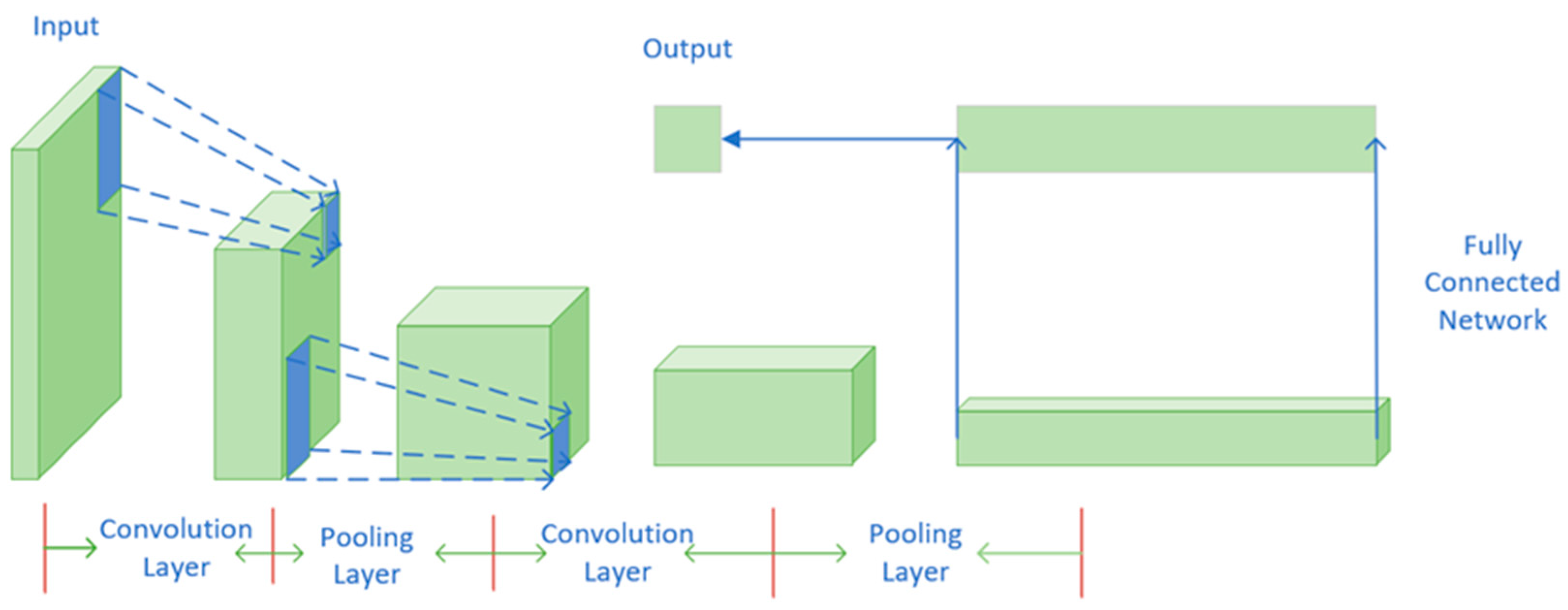
2.1. CNN Model

CNN is a deep learning model that has been widely used in several fields, such as image recognition, computer vision, and natural language processing. Inspired by the biological vision system, CNN uses multilayer convolution and pooling operations to automatically learn and extract features from input data.

The CNN training process typically utilizes techniques such as backpropagation to optimize the model. During training, CNN calculates losses by comparing predictions to true labels. It subsequently updates network parameters using optimization algorithms like gradient descent. This iterative process allows the model to gradually converge and improve prediction accuracy.

CNN has achieved great success in image and text processing through its ability to learn local perception through convolutional and pooling operations, the effectiveness of parameter sharing, and the representational capabilities of fully connected layers. These advantages enable CNN to automatically learn high-level feature representations from raw inputs, thus facilitating accurate modeling and analysis of complex data.

The basic components of a CNN include convolutional layers. Here are the functions and characteristics of each component in Figure 1:

• Convolutional layer: The convolutional layer is the core of CNN. It performs convolution operations by sliding a learnable convolutional kernel over the input data and applying a nonlinear activation function to the result. The convolution operations capture the local spatial relationships in the input data, extracting visual features in images or local structures in text. The parameter sharing mechanism of convolutional kernels reduces the number of parameters in CNN, making it less complex when dealing with a large number of inputs;
• Pooling layer: The pooling layer usually follows the convolutional layer. Its purpose is to reduce the dimensionality of feature maps, thus reducing the complexity of the model and preserving important features. Common pooling operations include max pooling and average pooling. Pooling operations aggregate values within a fixed-size window sliding over the input data, producing pooled results. This reduces the size of feature maps while providing some degree of translational and scale invariance;
• Fully connected layer: After convolution and pooling layers, features are flattened and connected to fully connected layers. A fully connected layer is a traditional neural network layer in which each neuron is connected to all neurons in the previous layer. It performs nonlinear mapping and classification tasks by learning weights and biases. Through multiple iterations of training, the fully connected layers can learn complex feature representations in high-dimensional space to classify or regressively predict input data.

2.2. GRU Recurrent Neural Network Model

GRU is designed to address the issues of vanishing and exploding gradients in traditional recurrent neural networks while maintaining strong modeling capabilities. Compared to other recurrent units like LSTM, GRU has a simpler structure with fewer parameters, making it more computationally efficient. The core idea of GRU is to introduce two gates, namely the Update Gate and Reset Gate, to control the flow of information within the network. At each time step, the GRU unit calculates the hidden state based on the current input, the previous hidden state, and the outputs of the gates. The steps are as follows:

• Reset Gate: The current input and the previous hidden state are concatenated and fed into a sigmoid activation function, producing a reset gate value between 0 and 1. It determines how much of the past information should be ignored;
• Update Gate: Similarly, the current input and the previous hidden state are concatenated and passed through a sigmoid activation function, generating an update gate value between 0 and 1. It determines how much of the new information should be included in the hidden state;
• Candidate Hidden State: the current input and the previous hidden state are concatenated and processed by the tanh activation function, resulting in a candidate hidden state value between −1 and 1;
• Updated Hidden State: Based on the update gate, candidate hidden state, and previous hidden state, a weighted sum operation is performed to obtain the current hidden state. The update gate controls the balance between the past and new information.

By incorporating reset and update gates, GRU can capture long-term dependencies in sequences and alleviate the vanishing gradient problem. Compared to LSTM, GRU has a simplified structure that is easier to train and optimize, particularly on smaller datasets. In summary, GRU is a commonly used recurrent unit for modeling sequential data. It introduces update and reset gates to improve long-term dependency modeling and offers higher computational efficiency compared to LSTM. The GRU structure is illustrated in Figure 2:

As shown in Figure 1, $r_t$ is the reset gate, $Z_t$ is the update gate, $X_t$ is the input at the current moment, and $h_t$ and $h_{t-1}$ are the outputs at the current and previous moments. The GRU parameters are calculated as follows:

$$z_t=\sigma (W_z\cdot [h_{t-1},x_t]),$$

(1)

$$r_t=\sigma (W_r\cdot [h_{t-1},x_t]),$$

(2)

$${\tilde{h}}_t=\tanh (W\cdot [r_t\ast h_{t-1},x_t]),$$

(3)

$$h_t=(1-z_t)\ast h_{t-1}+z_t\ast {\tilde{h}}_t,$$

(4)

where ${\tilde{h}}_t$ is the candidate hidden state; $W_z$, $W_r$, $W$ are the parameter matrices; and denotes $\sigma (x)$ and $\tanh (x)$ are the sigmoid and tanh activation functions.

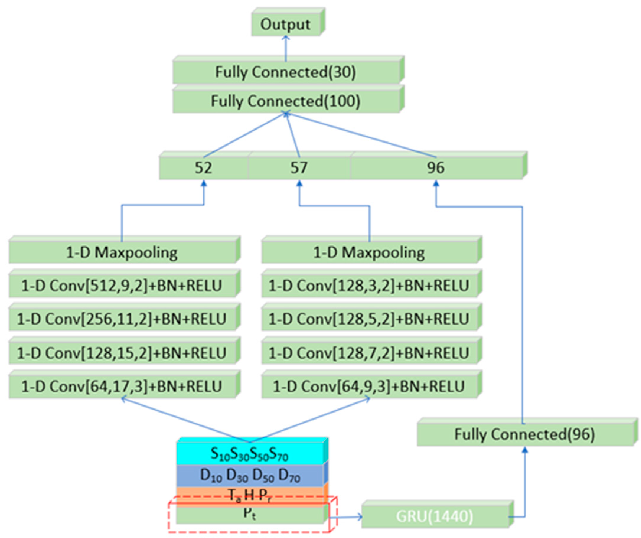
2.3. Multichannel-Based CNN–GRU Prediction Models

Regarding wind power, we form a feature matrix. This matrix merges 12 channels of data related to wind speed, wind direction, climate conditions, and past power readings. These data include 10 m, 30 m, 50 m, and 70 m wind speeds, 10 m, 30 m, 50 m, and 70 m wind directions, temperature, pressure, humidity, and past power readings. The time scale for each data type is one minute. These data points are combined over a time frame into a window of size $n$ = 1440, resulting in a 12 × 1440 matrix. Based on the multichannel CNN–GRU prediction model, features from the original feature matrix are extracted through three branches of processing, as shown in Figure 3:

• Left branch: This branch uses convolutional operations to extract global features from every data channel. For clarity, the first layer of one-dimensional convolution here has 64 kernels, each 17 in size, and operates at a step size of 3;
• Right branch: Here, partial features from each data channel are extracted using more compact convolution kernels. The first layer of one-dimensional convolution here has 64 kernels, each 9 in size, and operates at a step size of 3. This smaller kernel ensures finer feature extraction of subtle features;
• GRU neural network module: Input the past wind power generation outputs into a GRU neural layer, as indicated by the red box in Figure 2. This allows us to extract temporal features and capture the sequential traits of wind power generation. This extracts the temporal features. Following this, a fully connected layer pinpoints the time series traits, aiding in better understanding and predicting the trends of wind power generation. After this, features from global, partial, and temporal features are merged. This combined data is then run through a fully connected layer to determine the prediction result. Through this design, we make full use of global information, partial features, and temporal trends, enhancing the accuracy and reliability of the prediction model.

3. Results and Discussion of Prediction Models

To validate the accuracy of the predictive method proposed in this paper for wind power plant output prediction in practical applications, experimental verification was conducted using data collected from a wind power plant in Sichuan Province over the course of one year in 2020. The dataset consists of 1440 data points per day for each influencing factor and wind power output, collected at 1 min intervals. These data are classified into four main categories: wind speed, wind direction, weather, and historical output, as illustrated in Figure 4, Figure 5, Figure 6 and Figure 7, respectively. Their characteristics are shown in

Table 1. Characteristics of various factors.

Influencing Factor	Max	Min
Wind speed (m/s)	18	0
Wind direction (°)	360	0
Temperature (°C)	24	−11
Air pressure (Pa)	701	691.15
Humidity (%)	100	18.46
History contribution (kW)	90.02	0

. For model training, 70% of the complete dataset is employed, with 25% reserved for validation, and the remaining 5% designated for prediction.

Experimental Environment: We carried out the simulations on an Intel (R) Core (TM) i5-8250U processor. The algorithm model was built using the Python 3.7 language. To show the effectiveness of the CNN–GRU prediction model based on multichannel signals proposed in this paper, we compared it to other models for verification. These included the GRU model, LSTM model, Mutual Information Theory–LSTM model (MI–LSTM), and the Principal Component Analysis–LSTM model (PCA–LSTM). All these models were adjusted to operate at their best performance. To elaborate: the GRU model had three GRU units, the LSTM model had three LSTM units, and both the MI–LSTM and PCA–LSTM had three LSTM units. The PCA–LSTM model had its reference dimension set at 75%.

3.1. Multichannel Signal Construction

Wind power generation is inherently unpredictable due to the intricate interplay of multiple factors. The relationship expression between wind power and influencing factors is as follows:

$$P(x)=f(S_n,D_n,T_{\mathrm{a}},P_r,H,P_t),$$

(5)

where $P(x)$ is the wind power; $S_n$ is the wind speed; $D_n$ is the wind direction; $T_a$ is the air temperature; $P_r$ is the air pressure; $H$ is the humidity; and $P_t$ is the historical wind power.

The pivotal elements influencing wind power exhibit dependency on diverse meteorological conditions. Leveraging real-time meteorological data garnered from wind farms, a meticulous multichannel signal profile has been constructed to explicate the multifaceted factors impacting wind power.

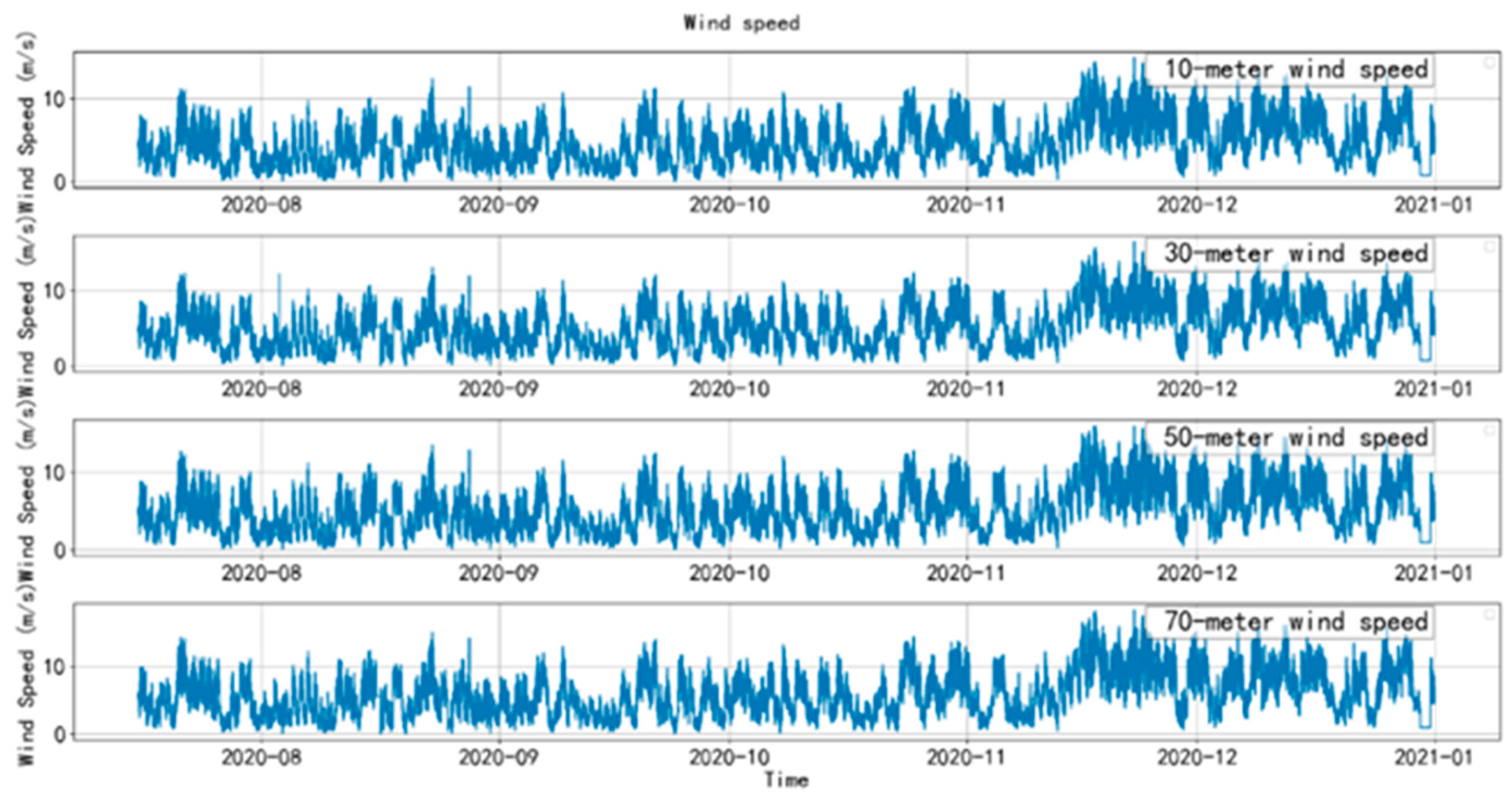
• Anemometer tower wind speed signal: Wind speed directly influences the amount of wind power generated. From observations at wind farms, wind speed data falls into four categories: 10 m, 30 m, 50 m, and 70 m wind speeds;
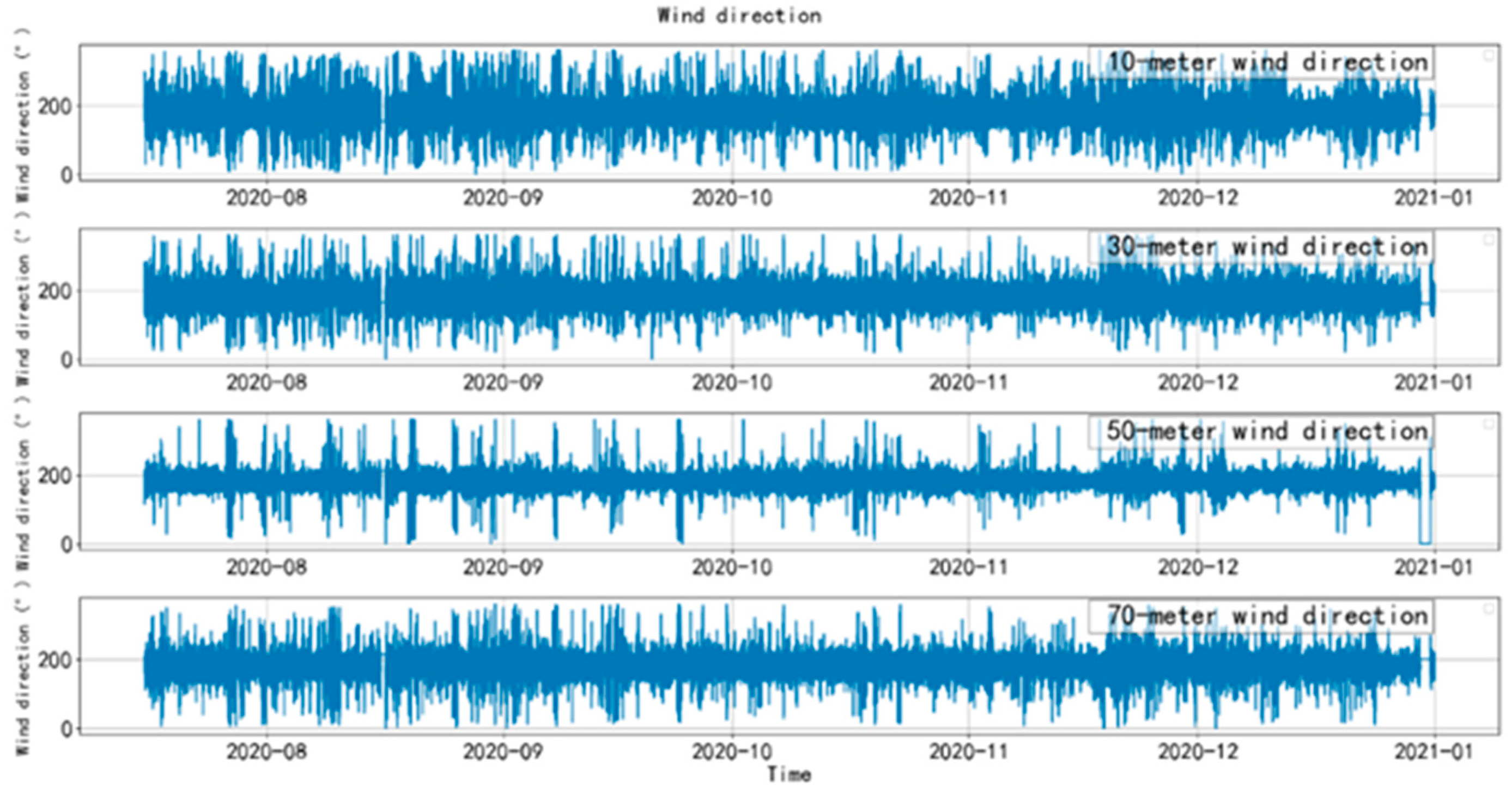
• Anemometer tower wind vane signal: The wind’s direction and its force on turbine blades determine the wind energy conversion rate. There are four main wind direction data types: 10 m, 30 m, 50 m, and 70 m wind directions;
• Wind tower climate monitoring signal: current weather elements, such as temperature, air pressure, and humidity, influence wind turbine output;
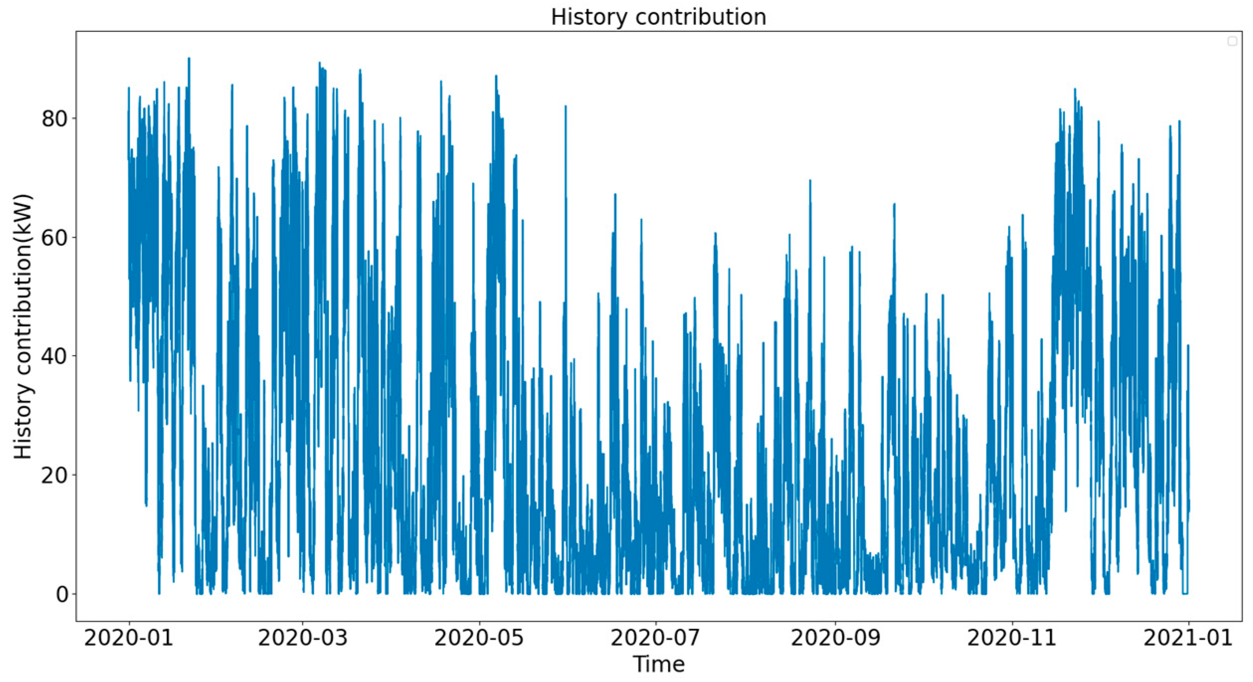
• Wind turbine output signal: The wind turbine output signal exhibits strong time series characteristics, allowing the model to learn from the temporal patterns of load variations through the time series data. This enables the model to capture the dynamic behavior and changes in wind power over time.

The partial features of the multichannel signals are collected from various channels within the wind farm, as shown in

Table 2. Multichannel signal summary.

Influencing Factors	Type of Feature	Feature Representation
Wind speed	10 m wind speed	S10
	30 m wind speed	S30
	50 m wind speed	S50
	70 m wind speed	S70
Wind direction	10 m wind direction	D10
	30 m wind direction	D30
	50 m wind direction	D50
	70 m wind direction	D70
Climate	Temperature	Ta
	Air pressure	Pr
	Humidity	H
History contribution	Wind power	Pt (1, 2, 3 … n)

. These multichannel signals serve as the model input, allowing it to extract the impact features of wind power generation effectively. An in-depth analysis of these features results in a comprehensive comprehension of the inherent unpredictability of wind power generation. Additionally, it furnishes valuable insights for the enhancement of the model.

3.2. Determination of the Prediction Window

The prediction capability of the model is determined by its prediction window size. Such capability is measured by how accurately it can forecast future periods over extended durations. In our experiment, we used prediction windows that spanned 15 min each. We tested various window lengths: two, three, four, five, six, and seven. For these window sizes, we employed different models to predict wind power. To assess the prediction accuracy of the model, we chose R2 and MSE as our evaluation indicators. The details of these indicators are provided below:

$$R^2=1-\frac{{\displaystyle {\sum }_{i=1}^n{(y_i-{\widehat{y}}_i)}^2}}{{\displaystyle {\sum }_{i=1}^n{(y_i-\overline{y})}^2}},$$

(6)

$$MSE=\frac{1}{n}{\displaystyle {\sum }_{i=1}^n{(y_i-{\widehat{y}}_i)}^2},$$

(7)

where $N$ denotes the data length; $y_t$ denotes the true value; ${\widehat{y}}_t$ denotes the load model calculated value; and $\overline{y}$ denotes the mean of true values.

According to

Table 3. Comparison of prediction accuracy in different windows.

Number of Windows	Evaluation Indicators	GRU	LSTM	MI– LSTM	PCA– LSTM	Methodology for This Paper
2	R2	0.9443	0.9445	0.9503	0.9517	0.9613
	MSE	0.0021	0.0030	0.0019	0.0015	0.0009
3	R2	0.9489	0.9499	0.9495	0.9501	0.9609
	MSE	0.0021	0.0019	0.0025	0.0018	0.0011
4	R2	0.9339	0.9329	0.9389	0.9432	0.9589
	MSE	0.0049	0.0051	0.0039	0.0031	0.0019
5	R2	0.9259	0.9267	0.9329	0.9331	0.9450
	MSE	0.0078	0.0071	0.0044	0.0048	0.0028
6	R2	0.8891	0.8901	0.8993	0.9011	0.9321
	MSE	0.0115	0.0099	0.0105	0.0095	0.0055
7	R2	0.8709	0.8711	0.8809	0.8891	0.9009
	MSE	0.0148	0.0145	0.0128	0.0108	0.0098

and Figure 8, our proposed method performed better than other models in terms of R2 and MSE. Even when the prediction window size increased, our method continued to exhibit superior performance. Additionally, it was more consistent, and its performance decline over time was comparably more gradual.

3.3. Ablation Experiments

This paper introduces a prediction model. This model has three feature extractors: two are CNN modules, and one is a GRU module. Accordingly, it is necessary to evaluate the impact of each feature extractor on the predictions. Thus, we adopt the same network parameters as shown in the CNN–GRU prediction model with multichannel signals as shown in Figure 3. These parameters are divided into three parts:

• Left branch for global feature extraction using CNN (global);
• Middle branch for partial feature extraction using Conv (partial);
• Right branch for time series extraction using GRU.

We first trained each module individually and produced predictions. Next, we combined modules in pairs and trained them. Thereafter, we compared the prediction accuracy of the six different configurations across prediction windows of sizes (five, seven, and nine). The results are displayed in

Table 4. Comparison of ablation experiment results.

Modules	Evaluation Indicators	Five Windows	Seven Windows	Nine Windows
Conv (Global)	R2	0.8835	0.8635	0.8495
	MSE	0.0137	0.0277	0.0393
Conv (Partial)	R2	0.8995	0.8766	0.8544
	MSE	0.0112	0.0199	0.0352
GRU (Temporal)	R2	0.8972	0.8663	0.8507
	MSE	0.0126	0.0224	0.0383
Conv (Global) + Conv (Partial)	R2	0.9344	0.9143	0.8992
	MSE	0.0041	0.0071	0.0116
Conv (Global) + GRU (Temporal)	R2	0.9309	0.9201	0.9005
	MSE	0.0043	0.0061	0.0099
Conv (Partial) + GRU (Temporal)	R2	0.9350	0.9250	0.9150
	MSE	0.0038	0.0052	0.0079

.

Table 4 proves the prediction accuracy for the three distinct modules and their combinations across window sizes of five, seven, and nine. Upon analysis, it becomes clear that relying solely on individual modules—be it Conv (Global), Conv (Partial), or GRU (Temporal)—falls short in feature extraction. This deficiency leads to less than optimal prediction accuracy. Interestingly, merging two modules elevates prediction accuracy. In addition, when the GRU (Temporal) module is absent, model accuracy experiences a steeper decline as the prediction sequence grows. This pattern suggests that the GRU (Temporal) module is finely attuned to extended time sequences and exhibits greater stability. Utilizing CNN for both global and partial feature extraction in the multichannel design and subsequently integrating this information through fully connected layers enriches the model’s ability. It becomes adept at illustrating the interconnections among diverse influencing factors. Therefore, the model devised in this study capitalizes on blending channel features with temporal elements. This holistic approach ensures that the collected data from the wind farm is fully utilized to optimize wind power generation predictions.

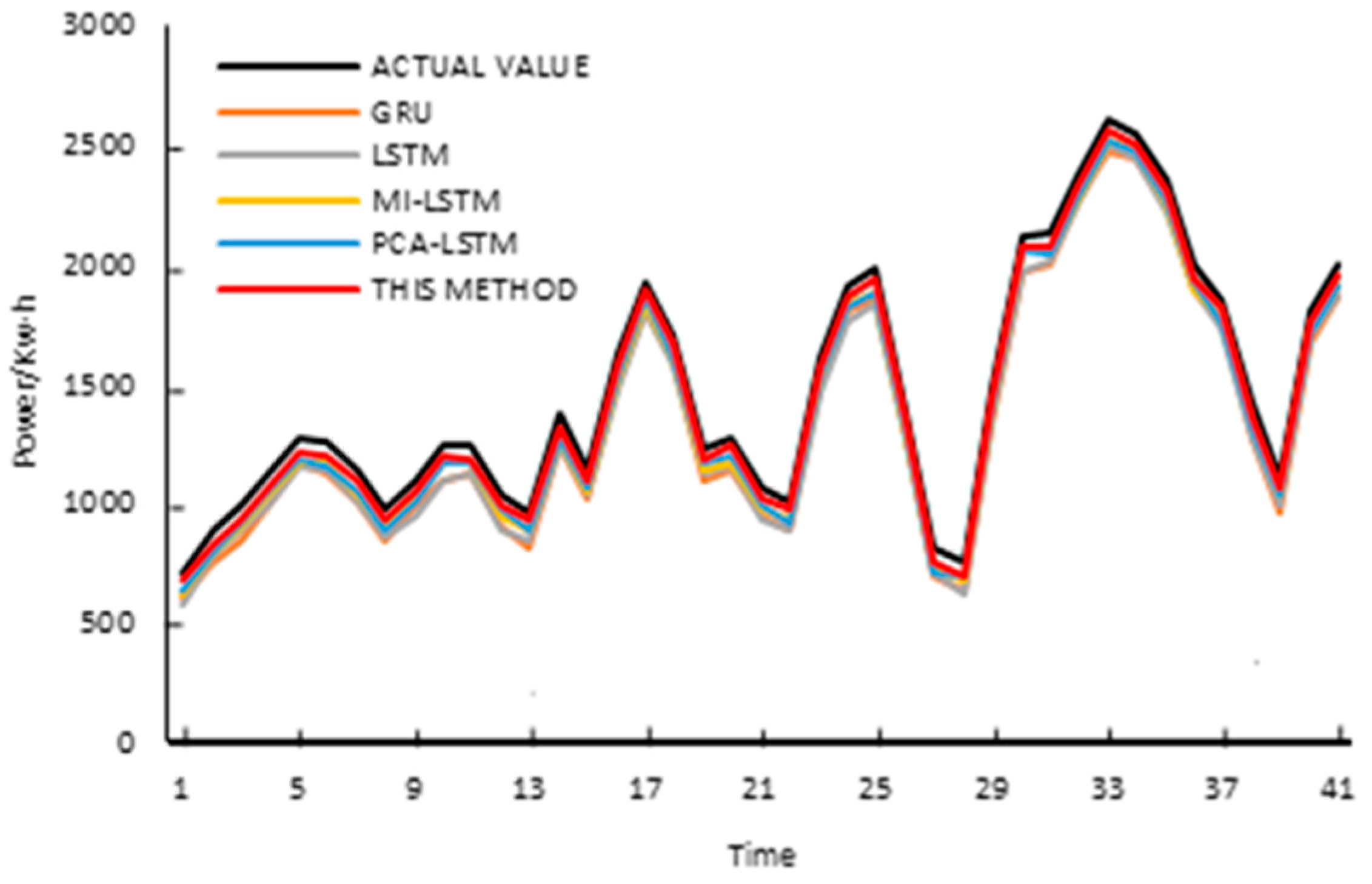
3.4. Open Data Set Trials

Regarding the data sources, this research employed historical datasets sourced from six wind power installations situated in Texas, USA. The data, provided by the National Renewable Energy Laboratory (NREL), covers the period between 2004 and 2006. They include both operational figures and associated influential elements, sampled at consistent 15 min intervals. Each unique ID number represents a different wind farm, and

Table 5. Specific locations of six wind farms.

ID	Latitude	Longitude
SITE_00173	36.14	−100.34
SITE_00193	36.42	−100.44
SITE_00215	36.42	−100.67
SITE_00365	36.50	−100.68
SITE_00446	36.50	−100.28
SITE_00797	36.56	−100.54

displays the specific locations of the wind farms.

Table 5 demonstrates the locations of the six wind power plants. Notably, they are situated close to each other. As a result, data from all six plants were combined for the purposes of model training. This combined dataset was then split: 70% was designated for training, and the remaining 30% for testing. Building on insights from Section 3.3, we established a prediction window size of seven. The same training parameters were applied to glean the training outcomes. The comparative results for each model are presented in both Figure 9 and

Table 6. Comparison of evaluation indicators among different models.

Models	R2	MSE
GRU	0.8696	0.0148
LSTM	0.8713	0.0141
MI–LSTM	0.8831	0.0125
PCA–LSTM	0.8873	0.0104
Proposed method	0.9013	0.0096

.

Based on the findings of Figure 8 and Table 6, it is evident that our method demonstrates superior prediction accuracy when trained on the public dataset. This indicates that our model possesses strong generalization capabilities on real-world data and effectively captures associations and trends within the data. These findings further validate the reliability and effectiveness of our approach, showcasing potential applications in wind power prediction.

4. Conclusions

This paper introduces a prediction model, specifically a CNN–GRU ultra-short-term wind power prediction model based on multichannel signals. CNN plays a pivotal role in extracting both global and partial features from the multichannel data collected by the power plant, while GRU networks are used to extract temporal features of historical wind power. These extracted features are then combined using a fully connected network to obtain predicted results. The proposed model offers several advantages:

• A multichannel data sample set includes wind speed, direction, air temperature, air pressure, humidity, and historical output. Such an approach ensures that data from wind farms is maximized. By leveraging CNN, both global and partial features are extracted from each channel. This process allows for the identification of key impact features associated with wind power generation;
• The GRU network, renowned for its capability to capture temporal dependencies in time series data, is pivotal to this paper. It adeptly extracts the historical temporal features of wind power.

Despite the significant progress achieved in this study, we acknowledge certain limitations. Specifically, the multichannel data utilized may have gaps in certain aspects. It does not comprehensively consider static characteristics, such as terrain and the size of wind farms, both of which can influence wind power output. Therefore, future studies should aim to supplement the dataset with additional static data from each wind farm. In this light, we hope to discover a wider range of factors that can influence wind power, so that the accuracy of the prediction models can be further improved.

References

1. Zhu, F.; Xu, J.; Pan, C.; Wang, C.; Zhao, X.; Tian, W. Coal carbon neutral goal in the opportunities and challenges. Electr. Power Technol. Environ. Prot. 2022, 38, 79–86. [Google Scholar]
2. Wang, W.; Wang, Z.; Dong, C. Status and error analysis of short-term forecasting technology of wind power in China. Autom. Electr. Power Syst. 2021, 45, 17–27. [Google Scholar]
3. Ye, L.; Zhao, Y. A review on wind power prediction based on spatial correlation approach. Autom. Electr. Power Syst. 2014, 38, 126–135. [Google Scholar]
4. Qin, C.; Yu, Y. Security region based probabilistic small signal stability analysis for power systems with wind power integration. Autom. Electr. Power Syst. 2014, 38, 43–48. [Google Scholar]
5. Ye, L.; Lu, P.; Zhao, Y.; Bai, B.; Yang, Y. Review of Model Predictive Control for Power System with Large-scale Wind Power Grid-connected. Proc. CSEE 2021, 41, 6181–6198. [Google Scholar]
6. Zhu, Q.; Li, J.; Qiao, J.; Shi, M.; Wang, C. Application and Prospect of AI Technology in Renewable Energy Forecasting. Proc. CSEE 2022, 2022, 1–23. [Google Scholar]
7. Zhang, Y.; Qiu, R.; Yang, F.; Xu, S.; Shi, X.; He, X. Overview of Application of Deep Learning with Image Data and Spatio-temporal Data of Power Grid. Power Syst. Technol. 2019, 43, 1865–1873. [Google Scholar]
8. Du, G.; Zhao, D.; Liu, X. Research review on optimal scheduling considering wind power uncertainty. Proc. CSEE 2022, 2022, 1–21. [Google Scholar]
9. Sun, R.; Zhang, T.; He, Q.; Xu, H. Review on Key Technologies and Applications in Wind Power Forecasting. High Volt. Eng. 2021, 47, 1129–1143. [Google Scholar]
10. Wang, T.; Gao, J.; Wang, Y.; Shi, Z.; Liu, T.; Yang, B.; Yan, F. Wind power prediction based on improved empirical mode decomposition and support vector machine. Electr. Meas. Instrum. 2021, 58, 49–54. [Google Scholar]
11. Xie, R.C.; Galer, S.J.; Abouchami, W.; Frank, M. Limited impact of eolian and riverine sources on the biogeochemical cycling of Cd in the tropical Atlantic. Chem. Geol. 2019, 511, 371–379. [Google Scholar] [CrossRef]
12. Jiang, J.; Wang, F.; Rui, T.; Zhang, L.; Xu, X. TS_XGB: Ultra-Short-Term Wind Power Forecasting Method Based on Fusion of Time-Spatial Data and XGBoost Algorithm. Procedia Comput. Sci. 2022, 199, 1103–1111. [Google Scholar]
13. Yu, Z.; Liu, X.; Yan, K.; Song, Y.; Zhou, K. Combination Model of Chance-constrained Security Constraint Unit with Considering the Forecast Uncertainties of DLR and Wind Power. High Volt. Eng. 2021, 47, 1204–1214. [Google Scholar]
14. Miao, C.; Li, H.; Wang, X.; Han, L.; Ma, Y.; Li, H. Data-driven and Deep-learning-based Ultra-short-term Wind Power Prediction. Autom. Electr. Power Syst. 2021, 45, 22–29. [Google Scholar]
15. Zhou, H.; Zeng, J.; Wang, Z.; Zhao, Q. Ridgelet neural network model for short-term wind power forecasting based on the combination of chaos DNA genetic and particle swarm optimization algorithm. Power Syst. Prot. Control 2013, 41, 144–149. [Google Scholar]
16. Zhang, Q.; Tang, Z.; Wang, G.; Yang, Y.; Yao, T. Ultra-short-term wind power prediction model based on long and short term of memory network. Acta Energiae Solaris Sin. 2021, 42, 275–281. [Google Scholar]
17. Ewees, A.A.; Al-qaness, M.A.; Abualigah, L.; Abd Elaziz, M. HBO-LSTM: Optimized long short-term memory with heap-based optimizer for wind power forecasting. Energy Convers. Manag. 2022, 268, 116022. [Google Scholar] [CrossRef]
18. Yang, M.; Peng, T.; Su, X. Ultra-short Term Wind Power Prediction Based on Two-dimensional Coordinate Dynamic Division of Prediction Information. Proc. CSEE 2022, 2022, 1–11. [Google Scholar]
19. Wang, Y.; Xie, D.; Wang, X.; Li, G.; Miao, Z.; Yu, Z. Prediction of Interaction Between Grid and Wind Farms Based on PCA-LSTM Model. Proc. CSEE 2019, 39, 4070–4081. [Google Scholar]
20. Wang, Y.; Chen, Y.; Han, Z.; Zhou, D.; Bao, Y. Short-term wind speed forecasting Model Based on mutual information and recursive neural network. J. Shanghai Jiao Tong Univ. 2021, 55, 1080–1086. [Google Scholar]
21. Niu, Q.; Li, X. A High-performance Web Attack Detection Method based on CNN-GRU Model. In Proceedings of the 2020 IEEE 4th Information Technology, Networking, Electronic and Automation Control Conference (ITNEC), Chongqing, China, 12–14 June 2020; pp. 804–808. [Google Scholar]
22. Kaselimi, M.; Doulamis, N.; Voulodimos, A.; Doulamis, A.; Delikaraoglou, D. Spatio-Temporal Ionospheric TEC Prediction Using a Deep CNN-GRU Model on GNSS Measurements. In Proceedings of the 2021 IEEE International Geoscience and Remote Sensing Symposium IGARSS, Brussels, Belgium, 11–16 July 2021; pp. 8317–8320. [Google Scholar]
23. Khan, I.; Maniraj, S.P.; Reddy, K.S.; Balaji, V.; Kalaivani, K.; Singh, M. Congenital Heart Disease Prediction based on Hybrid Approach of CNN-GRU-AM. In Proceedings of the 2023 7th International Conference on Intelligent Computing and Control Systems (ICICCS), Madurai, India, 17–19 May 2023; pp. 613–618. [Google Scholar]
Figure 1. Diagram of the basic component structure of CNN.
Electronics 12 04479 g001
Figure 2. Structure of the GRU model.
Electronics 12 04479 g002
Figure 3. Schematic diagram of a multichannel CNN–GRU prediction model.
Electronics 12 04479 g003
Figure 4. Wind speed data.
Electronics 12 04479 g004
Figure 5. Wind direction data.
Electronics 12 04479 g005
Figure 6. Climate data.
Electronics 12 04479 g006
Figure 7. History contribution data.
Electronics 12 04479 g007
Figure 8. Comparison of model prediction accuracy.
Electronics 12 04479 g008
Figure 9. Comparison results for each model.
Electronics 12 04479 g009