Abstract
Distributed power supplies have gradually become a new trend in power supply development, but access to a large number of distributed energy sources has a certain impact on the stable operation of the power grid. A virtual power plant (VPP) can integrate a variety of distributed power sources for coordination and optimization; thus, it can effectively solve the difficulties faced by a distributed energy grid connection and promote the complementarity of energy sources. However, renewable energy often has a degree of volatility and randomness when distributed, which can bring certain risks to the operation of the VPP. In order to consider the risks brought by renewable energy, an optimal scheduling model of the VPP, based on an improved generative adversarial network (GAN) and the conditional value at risk (CVaR), was proposed to measure the relationship between the benefits and risks. Firstly, the uncertainty of new energy is analyzed, and wind power and photovoltaic scenarios are generated by the improved GAN; then, typical scenarios are generated by the k-medoids method. Finally, based on the CVaR, the optimal scheduling model of the VPP is established to study the effect of risk weight on VPP revenue. The results show that the model can effectively measure the relationship between the benefits and risks and can provide some references for the VPP to make reasonable operational decisions with different risk preferences.
1. Introduction
With the rapid development of renewable energy power generation technology, a large amount of renewable energy continues to pour into the grid. However, at the same time, there are still great challenges in the construction of the energy internet [1,2,3,4]. Firstly, there is a large amount of uncertain wind power and photovoltaic power, due to the fact that the distributed power supply access to the current power system is dominated by thermal power generation; consequently, there is a considerable degree of difficulty involved in the coordination of traditional thermal power units and wind power output. Secondly, considering the integrated distributed energy system of wind power, photovoltaic power, thermal power, and other energy sources, each energy internet system operates independently of the others, due to geographical location and other factors, and lacks coordinated scheduling, resulting in a low level of resource utilization. Thirdly, the current power grid is increasingly large and faces a large amount of uncertain new energy integration, further increasing the complexity of the power system.
The VPP can manage the distributed energy in a certain area through information, control, communication, and other technologies; it can effectively connect to the power grid, alleviate the uncertain impact of various distributed resources on the safe and stable operation of the power system, promote the rational utilization of resources, and effectively meet the requirements of energy conservation, consumption reduction, and comprehensive energy utilization rate improvement [5,6,7,8].
In view of the uncertainty of the new energy output, the Monte Carlo method was used in [9] to solve the random characteristics of renewable energy power generation, and a two-stage random bidding strategy was proposed to maximize the daily profit of a VPP by considering the opportunity constraints. In [10], the Latin hypercube sampling method was adopted to solve and improve the uncertainty problem, speeding up the sampling speed and effectively improving the operating efficiency of the model. The authors of [11] used a Latin hypercube to simulate wind power and photovoltaic scenarios; then, the improved Clustering Large Applications (CLARA) algorithm was used to reduce the scenarios. Finally, the carbon trading mechanism was introduced to establish the optimal VPP scheduling model, with the goal of maximizing revenue.
As an important solution of distributed energy and grid-connected renewable energy management, VPP technology is receiving attention from countries all over the world [12]. Overall, the current technical research mainly focuses on the two categories of optimal scheduling and market bidding [13,14]. The former mainly studies the purchasing and selling strategy declaration of the VPP under centralized power system dispatching, which is aimed at the maximization of the economic benefit, and internal multi-distributed energy coordination dispatching, which is aimed at the lowest operating cost [15]. For the latter, the main research is focused on optimizing the bidding strategy of the VPP by participating in the multi-trading varieties of the combined power market and the renewable energy market’s trading mechanism [16,17]. In terms of optimal scheduling, [18] integrated an energy storage system and a demand response into the VPP and established the day-ahead optimal scheduling model of the VPP by considering multiparty uncertainties. The results showed that the addition of a demand response could effectively reduce the cost of the VPP. In [19], photovoltaic units, wind power units, energy storage equipment, and cogeneration units were assembled into a VPP, and the optimal scheduling model of the VPP was established with the goal of maximum revenue and minimum emissions, while considering the peak and valley electricity prices. The authors of [20] introduced carbon capture and waste incineration equipment to establish a VPP optimization scheduling model, and they used carbon capture equipment to smooth the fluctuations of the renewable energy units. The results showed that this model can effectively reduce the operating costs of the VPP and reduce carbon emissions. In terms of market bidding, [21] aggregated non-schedulable units, schedulable units, and an energy storage system as a VPP and studied the optimal bidding strategy of the VPP in the day-ahead market, real-time market, and rotating reserve market. The authors of [22] combined dispatchable units, non-dispatchable units, and dispatchable loads to build a VPP, and they introduced the information gap decision theory to deal with uncertainty and establish a VPP bidding decision model. In [23], a VPP was composed of renewable energy, conventional generator sets, and demand response, and a two-stage bidding strategy model for the VPP was established with the goal of maximizing revenue. The fuzzy optimization theory was introduced in the day-ahead stage, and the results showed that the model can effectively improve the profit of the VPP.
The above research shows that for the study of the uncertainty of new energy, most of the adopted simulation sampling methods were based on the Monte Carlo method and the Latin hypercube method. However, the above sampling methods usually relied on statistical assumptions, while only partial statistical information can be obtained from an actual project; so, it is difficult to obtain an accurate probability distribution. With the above methods, it has been difficult to meet the needs of the actual project; they have certain limitations and may deviate from the actual scenario. In addition, this uncertainty brings a great uncertainty risk to the VPP in the scheduling process, and a risk management method is urgently needed to measure the uncertainty. As a generative model, the GAN does not need to make any statistical assumptions about the distribution followed by the data, and it can directly learn from the data and generate new data samples, avoiding the establishment of probabilistic models; this can greatly improve the accuracy of scenario generation. The CVaR is a mathematical tool used to measure risk. In recent years, there have been many studies on the application of the CVaR in the related fields of the power system. Therefore, this paper combines the GAN and CVaR to analyze the optimal scheduling problem of the VPP. Firstly, the uncertainty of new energy is analyzed, and wind power and photovoltaic scenarios are generated by the improved GAN; then, typical scenarios are generated by the k-medoids method, which breaks the limitations of the simulation sampling methods in the above literature and effectively improves the accuracy of the generation scenarios. Finally, based on the CVaR, the optimal scheduling model of the VPP is established with the goal of maximum return; the relationship between return and risk is measured, the influence of risk weight on VPP return is studied, and the return of the VPP can be maximized under the condition of controllable risk.
2. Scenarios Generation Based on GAN
2.1. Improved GAN
The GAN is an unsupervised learning method, consisting of two modules, generator G and discriminator D [24,25,26,27]. Its main purpose is to conduct game training between the generator and discriminator to find the Nash balance. The basic structure of the GAN is shown in Figure 1. The generator is mainly responsible for capturing the probability distribution of real data and generating new samples through simulation. The discriminator is mainly responsible for distinguishing between the data, judging the similarity between the data generated by the generator and the real data, determining whether the input data are the real data, and outputting the probability that the data to be identified are the real data. Through continuous iterative training, the generator tries to accurately generate data that are basically the same as the real data, so that the discriminator cannot accurately judge the input data. In the training process, the generator and discriminator improve the generation ability and judgment ability through continuous optimization and finally achieve a Nash balance, so that the discriminator cannot accurately distinguish the generated data from the real data.
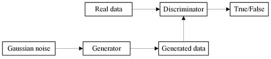
Figure 1.
Basic structure of GAN.
Let the real sample be and the noise be . The real samples are sampled in the data distribution, and the noise is sampled in Gaussian distribution . The noise is taken as the input data of the generator G, and the output generates data . The generated data distribution is . Real data are input into discriminator D; output represents the probability that are the real data. The loss function of both is shown below.
where is the generator loss function; is the discriminator loss function; is the expected distribution; is the probability of determining the generated data as real data after input into the discriminator.
The game training model of the generator and discriminator is shown below.
In order to better optimize the convergence effect and improve the accuracy of the results, the original GAN is improved, and the mean square error is introduced into the generator loss function.
where is the total number of samples.
In addition, since the original GAN uses Jensen–Shannon (JS) as a loss function in discriminator D, the problem of training instability easily occurs. Therefore, the Wasserstein distance [28,29] is introduced to measure the distance between the real data and the generated data distribution, and its definition is shown as follows:
where is the definite bound on the function value; is the Lipschitz constant; indicates that the discriminator D constitutive function must satisfy the K-Lipschitz continuity.
In order to improve the training speed, a penalty item is introduced. To sum up, the training model can be rewritten as the following formula:
where is the coefficient of the penalty term; is the gradient operator; and , .
At the beginning of the training, there is a big difference between the data generated by the generator and the real data, and the discriminator can easily distinguish between them. Then, through continuous optimization and training, the generative capacity and the discriminability of the generator and discriminator are continuously improved. It is difficult for the discriminator to distinguish the generated data from the real data. At this point, the model training is completed, and a set of wind power and photovoltaic data can be input for scenario generation.
2.2. Scenario Reduction Based on K-Medoids
The number of scenarios generated is too large, and there are a large number of similar scenarios; so, it is necessary to reduce the scenarios to obtain typical scenarios, so that one scenario can simulate the effect of multiple scenarios. At present, the rapid forward selection method, the synchronous back generation reduction method, and the scenario number construction method are mainly used for scenario reduction, but these methods have large computational quantities and are complex; so, this paper adopts the K-medoids method [30,31,32] to reduce the scenarios. The core idea of the K-medoids method is to divide the generated scenarios into several groups according to the degree of similarity and to choose one scenario in each group as a typical scenario. This ensures that after reduction, each scenario has its own characteristics and is representative and that the sum of the probability of the scenario after reduction is 1. The basic steps for the cutting scenarios using the K-medoids method are shown below.
Step 1: Randomly select m scenarios from the generated scenarios as the initial clustering center.
Step 2: Assign the remaining objects to each class according to the principle of being closest to the cluster center.
Step 3: According to the minimum distance principle of Equation (7), a new cluster center is found to replace the original cluster center:
where is the set of scenarios before cutting; is a collection of classic scenarios formed after scenario reduction; is the probability of the scenario appearing; and is the distance between any two scenarios , in the scenario set.
Step 4: Judge whether it converges. If it does not, repeat Step 2. If it does, the newly obtained m clustering centers are the reduced typical scenarios.
3. Optimal Scheduling Strategy of VPP Based on CVaR
3.1. Modeling of Components in VPP
In this paper, the wind turbine, photovoltaic unit, gas unit, energy storage equipment, and demand response resources are selected as the units in the VPP for analysis. The wind turbine and the photovoltaic turbine can convert solar energy and wind energy into electric energy, respectively. They are the main power generation members in the VPP. Photovoltaic power is mainly concentrated in the daytime, with certain fluctuations. Wind power output is produced in each period of a day, but the randomness is significant. The gas unit can output electricity stably and, to a certain extent, can calm the randomness of the wind and photovoltaic resources and realize the coordinated operation of the VPP. The main function of the energy storage device is to balance the wind power and photovoltaic resources in the VPP and provide a certain guarantee for the stable operation of the VPP. Demand response resources are managed via the signing of agreements with users through the means of a policy, allowing the VPP to control part of the load and to participate in the transaction.
3.1.1. Gas Unit
The operation constraints of the gas unit mainly include output constraints, climbing constraints, and start–stop constraints, as shown below.
where and are the lower limit and upper limit of the gas unit output, respectively; is a binary variable; is 0 indicates that the unit is in the running state; is 1 indicates that the unit is in the stopped state; and are the downward and upward climbing rates of the unit, respectively; and is the time from to .
3.1.2. Distributed Photovoltaic and Wind Turbines
As photovoltaic and wind power are both renewable energy sources, their power generation costs are low and can be considered to be zero. The pre-predicted available and actual output should meet the following constraints:
where and are, respectively, the upper limits of the available output predicted by the wind power and photovoltaic units; and are, respectively, the actual output upper limits of the wind power and photovoltaic units.
3.1.3. Energy Storage Equipment
The cost of the energy storage equipment is mainly the charge and discharge cost.
where and are the charging and discharging cost coefficients of the energy storage equipment, respectively.
The electric energy generated by the energy storage device is determined by its own running state. The mathematical expression is as follows:
where and are the charging and discharging efficiency factors, respectively; and are the charging and discharging power of the energy storage device, respectively.
During operation, the charging and discharging power and capacity must meet the following constraints:
where and are binary variables. When it is in a charge state, is 1; otherwise, it is 0; when it is in a discharge state, is 1; otherwise, it is 0; and are, respectively, the maximum charging and discharging power of the energy storage device; and are, respectively, the upper and lower limits of the energy storage equipment.
3.1.4. Demand Response
Demand response can adjust the behavior of the load side and guide the user side to optimize the VPP scheduling according to the needs of the system. This paper only considers the incentive demand response and control of the user load. Its mathematical model is as follows:
where is the demand response imposed on users at time ; is the user load at time ; is the proportion of the load in which users can participate in the demand response in the total load at time ; is the maximum demand response that can be imposed by the user.
3.2. Optimal Scheduling Model Based on CVaR
The first stage is the day-ahead declaration stage, where the VPP predicts the wind and solar power output and submits the day-ahead bidding output for each time period of the following day. After winning the bid, each unit will participate in dispatching power generation. In the second stage, after real-time updates, there may be deviations between the actual and predicted values of the wind and solar power output. The VPP uses equipment such as gas turbines and energy storage equipment to suppress deviations and compensates for the deviations that cannot be suppressed.
3.2.1. Objective Function
As the wind power and photovoltaic units in the VPP are characterized by volatility and randomness, to reduce the impact brought by volatility the CVaR was introduced in this paper to measure risk losses [33,34,35], balance risks and returns, and to maximize the returns. The CVaR is a commonly used risk measurement model. It can reduce the risks faced by decision makers in market competition by assessing risks and returns. The loss function of is set to be . For the determined , the probability value caused by not exceeding the critical value is shown below.
where is the decision variable; is a random variable; is the loss accumulation distribution function under .
For a given confidence coefficient , the value at risk, (VaR) is calculated as follows:
When the loss function is greater than or equal to , the CVaR value can be expressed as the following formula:
where .
Since is difficult to obtain, it needs to be discretized. The CVaR value obtained after the discretization result is substituted into Equation (23) is as follows:
where is the probability of scenario , and is the number of scenarios.
Accordingly, the optimal scheduling model of the VPP based on the CVaR is shown as follows. It is divided into two parts to maximize the profit. Part one is the expected profit under each scenario, which is represented by the profit from the electricity purchase and the sale minus the total cost of the VPP. The other part is the product of the risk weight and the CVaR, which is used to measure the risk.
where is the risk weight of the CVaR, ; the higher the value, the more serious the risk aversion; is the optimized running time; is the market revenue ahead of the time in scenario ; is the real-time market profit of the time in the scenario; is the total cost of the VPP; is the VaR value at the confidence coefficient ; is the auxiliary variable for calculating the CVaR.
where is the number of gas units; is the number of energy storage devices; and is the cost of imposing a demand response.
where and are the day-ahead market price and real-time market price in the time period, respectively; is the pre-date bidding effort in the time period; is the penalty coefficient; is the part that exceeds the bid; and is the part that is less than the bid.
3.2.2. Constraint Condition
- (1)
- Constraints of internal units
The constraints of the gas unit are shown in Equations (9)–(12). The distributed photovoltaic and wind turbine constraints are shown in Equations (13) and (14). The constraints of the energy storage equipment are shown in Equations (17) and (18). The constraint of the incentive demand response is shown in Equations (19) and (20).
- (2)
- Day-ahead bidding constraints
Before the power market closes, it is necessary to predict the available capacity in advance and to determine the bidding capacity before the date.
where is the number of wind turbines, and is the number of photovoltaic units.
- (3)
- Real-time market constraint
In a real-time market, gas units, energy storage equipment, and demand response are used to balance output deviations.
- (4)
- CVaR constraint
4. Integrated Scheduling Strategy
The overall scheduling strategy of this paper is shown in Figure 2. The first part uses a scenario generation method to solve the uncertainty of the new energy. The historical data were input into the improved GAN model to simulate a large number of output scenarios. Then, K-medoids were used to reduce the simulated scenarios to obtain representative typical scenarios. The second part is the optimal scheduling problem of the VPP. In the day-ahead stage, the next-day output of the VPP is predicted in advance to determine the declared purchased and sold electricity. In the real-time stage, gas units, energy storage equipment, and demand response resources are used to suppress the deviation caused by the wind and photovoltaic output; the part that cannot be suppressed is punished for the deviation. If the actual output is higher than the declared price, the electricity is sold at a price lower than the real-time electricity price; if the actual output is lower than the declared price, the electricity is bought at a price higher than the real-time electricity price. In order to measure the uncertainty risks, the CVaR was introduced to establish the optimal scheduling model of the VPP. With the goal of maximizing the benefits, the solution was carried out under the condition that the constraints had to be satisfied. Finally, the results were output.
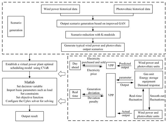
Figure 2.
Scheduling strategy of VPP based on improved GAN and CVaR.
5. Example Analysis
5.1. Basic Data
The structural diagram of the VPP is shown in Figure 3. The VPP selected in this paper contains three 2 MW wind turbines, four 2 MW photovoltaic turbines, a 4 MW gas turbine, and the energy storage equipment. The optimization duration is divided into 24 periods, i.e., 24 h. The cost of the demand response is 300 CNY/MW, and the maximum demand response applied is not more than 20% of the user load. The parameters of the gas units and energy storage equipment are shown in Table 1. The initial output power of the gas unit is 1.5 MW, and the initial capacity of the energy storage device is 6 . The user load curve and the electricity price curve are shown in Figure 4 and Figure 5, respectively. The penalty coefficient is 0.3, the confidence coefficient is 0.9, and the risk weights are 0.1, 0.5, and 0.9, respectively.
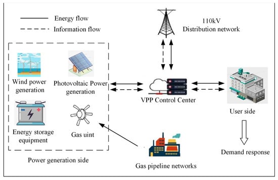
Figure 3.
The structure diagram of VPP.

Table 1.
Gas and energy storage equipment parameters.
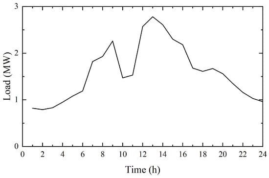
Figure 4.
User load curve.
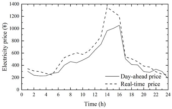
Figure 5.
Electricity price curve.
Firstly, the actual daily power generation of the wind and photovoltaic power is input into the model, generating 200 wind and photovoltaic scenarios through simulation. Then, the scenarios are reduced to five sets. Finally, the gas turbine, energy storage equipment, load, and electricity price data, as well as the five sets of scenario data just obtained, are input into the model; then, the final revenue result is output.
5.2. Result Analysis
5.2.1. Typical Scenarios Generation Based on Improved GAN and K-Medoids
The basic data of the output in this paper are from a set of wind power and photovoltaic output data of an industrial park in northeast China from 1 January 2020 to 30 December 2020. The data sampling interval is 1 h. A PyTorch framework was used to build the GAN, and 200 wind power and photovoltaic scenarios were generated. Then, MATLAB was used for the scenario reduction operations. Figure 6 shows the typical wind power and photovoltaic scenarios obtained after reduction. Table 2 shows the probability of the wind and photovoltaic scenarios; the probability of their combination scenarios is their product.
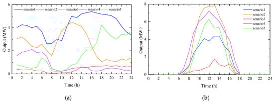
Figure 6.
The scenario after the reduction: (a) wind power scenario, (b) photovoltaic scenario.
Table 2.
The probability of wind and photovoltaic scenarios.
Figure 7 shows the training effect of the wind power and photovoltaic output under different iterations. It can be seen that in the early stage of the iterations, the generated scenario has not fully learned the characteristics of the wind power and photovoltaic output, and the effect is not so good. With the increase in the iterations, the generator gradually generates accurate wind power and photovoltaic scenarios through continuous learning. When the number of iterations reaches 500, the curve has learned the output characteristics; the generated curve is gradually smoothed, and the generator and discriminator basically reach the equilibrium state, generating the output scenario which conforms to the real rules. Figure 8 shows the cumulative distribution diagram of the real and generated scenarios of the wind power and photovoltaic output [36]. It can be seen that the probability distribution of the generated scenario and the real scenario is almost exactly the same, which proves the accuracy of the generated scenario.
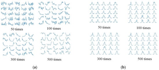
Figure 7.
A rendering of the scenario training: (a) wind power scenario, (b) photovoltaic scenario.
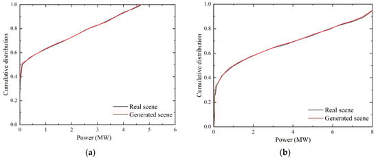
Figure 8.
Cumulative distribution: (a) wind power, (b) photovoltaic.
5.2.2. The Influence of Risk Weight on Each Unit Inside a VPP
Figure 9a,b describe the output of the wind power units and photovoltaic units under the different risk weights, respectively. It can be seen that the photovoltaic units only generate electricity during the day, while the wind power not only generates electricity during the day, but also generates electricity at night. Their output is complementary, which can effectively smooth the system fluctuations. In addition, the output of the wind power and photovoltaic units generally decreases with the increase in risk weight, indicating that VPPs are more inclined to use wind and photovoltaic units to participate in market competition when they have a risk preference, which can provide greater benefits, but at the same time has greater risks.
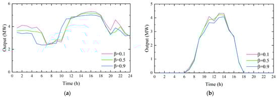
Figure 9.
The output of each unit of VPP under different risk weights: (a) wind power, (b) photovoltaic, (c) charging power of energy storage equipment, (d) discharging power of energy storage equipment, (e) gas unit, (f) demand response.
Figure 9c,d show the charging power and discharging power of the energy storage device. It can be seen that different risk weights have little influence on the charge and discharge of the energy storage equipment. The energy storage equipment mainly discharges in 6–10 h and 12–16 h and charges in the two periods of 2–5 h and 17–23 h. It can be seen from the electricity price curve that the price of 6–10 h and 12–16 h is relatively high, while the price of 2–5 h and 17–23 h is relatively low. This shows that the charge and discharge behavior of the energy storage equipment is mainly affected by the level of the electricity price. It has the characteristics of discharging at the peak stage of the electricity price and charging at the period of the low electricity price. It is flexible and operable.
Figure 9e,f show the output of the gas units and the demand response, respectively. It can be seen that the output of the gas units is mainly in the period of 6–9 h and 11–16 h, which is similar to that of the energy storage equipment to some extent. It can not only balance the output deviation caused by the uncertainty of the wind power output but can also produce electricity at the peak of the electricity price, sell electricity to the market, and shut down at a low price, which can improve the economic benefits of the VPP to a certain extent. In addition, with the increase in the risk weight, the output of the gas units is generally on the rise. This shows that in the case of risk aversion, the gas units are more inclined to participate in market transactions. The output of the demand response is related to the consumption behavior of the users, which is generally manifested as the demand response behavior imposed on the users during the peak hours of 6–9 h and 11–16 h.
5.2.3. The Relationship between CVaR and Profit
Table 3 shows the VPP revenue and CVaR values under different risk weights. As can be seen from the table, when the risk weight increases the total profit and CVaR value of the VPP decrease continuously. This shows that when the risk-bearing capacity of the VPP is weak, the utilization of the wind power and photovoltaic units is low; although the profit is small, the risk is also small. When the VPP has a strong risk tolerance, it can make more use of the wind power and photovoltaic units. Although the risk is higher, it will have a great profit at the same time.
Table 3.
VPP income and CVaR value under different risk weights.
5.2.4. Comparison between the Proposed Scheduling Model and the Traditional Scheduling Model
In order to analyze the rationality and robustness of the proposed scheduling model, set the risk weight to 0.1 and select the following models for comparison. (1) Use the model proposed in this article for scheduling based on Figure 5. (2) Select five other sets of scenarios again to schedule using the model in this article. (3) Use the predicted scenario as the traditional scheduling model for the wind and photovoltaic scenarios. The analysis results are shown in Table 4.
Table 4.
Model comparison result.
It can be seen from Table 4 that, compared with Model 1, the total profit of Model 3 is lower than that of Model 1. The reason is that Model 3 ignores the influence of the uncertainty of the wind power output. However, Model 1 fully considers the influence of the uncertainty; the addition of the CVaR in the model makes the total profit of Model 1 higher than that of Model 3. Therefore, it is proven that the VPP optimal scheduling model proposed in this paper can deal with the uncertainty risks more effectively and can maximize the benefits. At the same time, we can see that the total profits of Model 1 and Model 2 are both higher than that of Model 3. This indicates that the model proposed in this paper can effectively face uncertainty problems under different scenarios of renewable energy, proving the robustness of the model.
6. Conclusions
The optimal scheduling problem of the VPP was studied. Firstly, the uncertainty of the new energy was analyzed, and the improved GAN was used to generate wind power and photovoltaic scenarios; then, the K-medoids were used to reduce the scenarios and generate typical scenarios. Finally, based on the CVaR, the optimal scheduling model of the VPP was established with the goal of maximum profit. The influence of the different risk weights on the return of the VPP was analyzed, and the conclusions are as follows.
- (1)
- The improved GAN model can avoid the difficult problem of traditional probabilistic model establishment, and the probability distribution characteristics of the generated scenario are basically consistent with those of the real scenario, which can effectively solve the uncertainty problem of renewable energy.
- (2)
- Risk weight has a certain influence on each unit in the VPP. Among them, photovoltaic and wind turbines are more obvious. With the increase in the risk weight, the risk decreases, and the output of the photovoltaic and wind turbines decreases continuously. Energy storage equipment and gas units are utilized to balance the uncertainty deviation between the day-ahead bidding and the actual output to the maximum extent, and the method of “low charge and high discharge” and “high start and low stop” is adopted to obtain greater economic benefits in the real-time market.
- (3)
- The risk weight also has a certain effect on the income of the VPP. The higher the risk tolerance of the VPP, the greater the profit. Accordingly, schedulers can balance the risks and profits according to their risk aversion; they can determine the impact of the risks on scheduling decisions, formulate reasonable operation strategies, and obtain more benefits.
The paper achieved preliminary results in the study of the optimal scheduling of the VPP, but for the scenario generation part, this paper did not take the season and other factors into account, and the actual environment will have a certain impact on the scenario. In the future, quantitative analysis of the season and other factors should be carried out to improve the accuracy of the scenario generation. As for the optimal scheduling part, the energy storage devices considered in this paper are only limited to the power network. At the moment, cool and heat supplies and water networks can also be used as energy storage devices; electric vehicles are also connected to the power grid in large numbers. In the next step, cold storage, heat storage, pumped storage, and electric vehicles can be added to the optimization model of the VPP for further research.
Author Contributions
Conceptualization, Y.Z. and J.S.; methodology, Z.Z.; software, Z.Z.; validation, D.W., D.Z. and Z.Z.; formal analysis, D.W.; investigation, W.B.; resources, J.S.; data curation, W.B.; writing—original draft preparation, Z.Z.; writing—review and editing, D.W.; visualization, Z.Z.; supervision, Y.Z.; project administration, Y.Z.; funding acquisition, Y.Z. All authors have read and agreed to the published version of the manuscript.
Funding
This work was supported by the Applied Foundational Research Plan Project of Liaoning Province (2022JH2/101300218).
Data Availability Statement
Data sharing not applicable. No new data were created or analyzed in this study. Data sharing is not applicable to this article.
Conflicts of Interest
The authors declare no conflict of interest.
Abbreviations
| VPP | Virtual Power Plant |
| GAN | Generative Adversarial Network |
| CLARA | Clustering LARge Applications |
| VaR | Value at Risk |
| CVaR | Conditional Value of Risk |
| JS | Jensen–Shannon |
References
- Luo, L.; Abdulkareem, S.S.; Rezvani, A.; Miveh, M.R.; Samad, S.; Aljojo, N.; Pazhoohesh, M. Optimal scheduling of a renewable based microgrid considering photovoltaic system and battery energy storage under uncertainty. J. Energy Storage 2020, 28, 101306. [Google Scholar] [CrossRef]
- Zakaria, A.; Ismail, F.B.; Lipu, M.S.H.; Hannan, M. Uncertainty models for stochastic optimization in renewable energy applications. Renew. Energy 2020, 145, 1543–1571. [Google Scholar] [CrossRef]
- Shi, J.; Ma, L.; Li, C.; Liu, N.; Zhang, J. A comprehensive review of standards for distributed energy resource grid-integration and microgrid. Renew. Sustain. Energy Rev. 2022, 170, 112957. [Google Scholar] [CrossRef]
- Nunes, J.B.; Mahmoudi, N.; Saha, T.K.; Chattopadhyay, D. Multi-stage co-planning framework for electricity and natural gas under high re-newable energy penetration. IET Gener. Transm. Distrib. 2018, 12, 4284–4291. [Google Scholar] [CrossRef]
- Hooshmand, R.A.; Gholipour, E. A comprehensive review on microgrid and virtual power plant concepts employed for distrib-uted energy resources scheduling in power systems. Renew. Sustain. Energy Rev. 2017, 67, 341–363. [Google Scholar]
- Yin, S.; Ai, Q.; Li, Z.; Zhang, Y.; Lu, T. Energy management for aggregate prosumers in a virtual power plant: A robust Stackelberg game approach. Electr. Power Energy Syst. 2020, 117, 105605. [Google Scholar] [CrossRef]
- Alahyari, A.; Ehsan, M.; Mousavizadeh, M.S. A hybrid storage-wind virtual power plant (VPP) participation in the electricity markets: A self-scheduling optimization considering price, renewable generation, and electric vehicles uncertainties. J. Energy Storage 2019, 25, 100812. [Google Scholar] [CrossRef]
- Yang, D.; He, S.; Wang, M.; Pandžić, H. Bidding Strategy for Virtual Power Plant Considering the Large-Scale Integrations of Electric Vehicles. IEEE Trans. Ind. Appl. 2020, 56, 5890–5900. [Google Scholar] [CrossRef]
- Fu, H.; Wu, Z.; Zhang, X.P.; Brandt, J. Contributing to DSO’s Energy-Reserve Pool: A Chance-Constrained Two-Stage VPP Bidding Strategy. IEEE Power Energy Technol. Syst. J. 2017, 4, 94–105. [Google Scholar] [CrossRef]
- Ma, Z.; Gao, J.; Hu, W.; Dinavahi, V. Risk-adjustable stochastic schedule based on Sobol augmented Latin hypercube sampling consid-ering correlation Wind power uncertainties. IET Renew. Power Gener. 2021, 15, 2356–2367. [Google Scholar] [CrossRef]
- Cao, W.; Wang, S.; Xu, M. Optimal Scheduling of Virtual Power Plant Based on Latin Hypercube Sampling and Improved CLARA Clustering Algorithm. Processes 2022, 10, 2414. [Google Scholar] [CrossRef]
- Dehghan, M.; Zadehbagheri, M.; Kiani, M.J.; Nejatian, S. Virtual power plants planning in the distribution network constrained to system resiliency under extreme weather events. Energy Rep. 2023, 9, 4243–4256. [Google Scholar] [CrossRef]
- Kardakos, E.G.; Simoglou, C.K.; Bakirtzis, A.G. Optimal Offering Strategy of a Virtual Power Plant: A Stochastic Bi-Level Approach. IEEE Trans. Smart Grid 2016, 7, 794–806. [Google Scholar] [CrossRef]
- Li, B.; Yang, F.; Qi, B.; Bai, X.; Sun, Y.; Chen, S. Research on key technologies of P2P transaction in virtual power plant based on blockchain. IET Smart Grid 2022, 5, 223–233. [Google Scholar] [CrossRef]
- Khandelwal, M.; Mathuria, P.; Bhakar, R. Virtual Power Plant (VPP) scheduling with uncertain multiple Locational Marginal Prices. IET Energy Syst. Integr. 2022, 4, 436–447. [Google Scholar] [CrossRef]
- Hadayeghparast, S.; Farsangi, A.S.; Shayanfar, H. Day-ahead stochastic multi-objective economic/emission operational sched-uling of a large scale virtual power plant. Energy 2019, 172, 630–646. [Google Scholar] [CrossRef]
- Nguyen-Duc, H.; Nguyen-Hong, N. A study on the bidding strategy of the Virtual Power Plant in energy and reserve market. Energy Rep. 2020, 6, 622–626. [Google Scholar] [CrossRef]
- Zamani, A.G.; Zakariazadeh, A.; Jadid, S. Day-ahead resource scheduling of a renewable energy based virtual power plant. Appl. Energy 2016, 169, 324–340. [Google Scholar] [CrossRef]
- Pandey, A.K.; Jadoun, V.K.; Sabhahit, J.N. Real-Time Peak Valley Pricing Based Multi-Objective Optimal Scheduling of a Virtual Power Plant Considering Renewable Resources. Energies 2022, 15, 5970. [Google Scholar] [CrossRef]
- Zhang, Z.; Du, J.; Zhu, K.; Guo, J.; Li, M.; Xu, T. Optimization scheduling of virtual power plant with carbon capture and waste incineration considering P2G coordination. Energy Rep. 2022, 8, 7200–7218. [Google Scholar] [CrossRef]
- Vahedipour-Dahraie, M.; Rashidizadeh-Kermani, H.; Shafie-Khah, M.; Catalao, J.P.S. Risk-Averse Optimal Energy and Reserve Scheduling for Virtual Power Plants Incorporating Demand Response Programs. IEEE Trans. Smart Grid 2021, 12, 1405–1415. [Google Scholar] [CrossRef]
- Shafiekhani, M.; Ahmadi, A.; Homaee, O.; Shafie-Khah, M.; Catalão, J.P. Optimal bidding strategy of a renewable-based virtual power plant including wind and solar units and dispatchable loads. Energy 2021, 239, 122379. [Google Scholar] [CrossRef]
- Al-Awami, A.T.; Amleh, N.A.; Muqbel, A.M. Optimal Demand Response Bidding and Pricing Mechanism with Fuzzy Optimiza-tion: Application for a Virtual Power Plant. IEEE Trans. Ind. Appl. 2017, 53, 5051–5061. [Google Scholar] [CrossRef]
- Wei, H.; Hongxuan, Z.; Yu, D.; Yiting, W.; Ling, D.; Ming, X. Short-term optimal operation of hydro-wind-solar hybrid system with improved generative adversarial networks. Appl. Energy 2019, 250, 389–403. [Google Scholar] [CrossRef]
- Shuvendu, R. Applying Aging Effect on Facial Image with Multi-domain Generative Adversarial Network, International Journal of Image. Graph. Signal Process. 2019, 12, 14–22. [Google Scholar]
- Pham, T.T.; Pham, T.D.; Ta, V.C. Evaluation of GAN-based Models for Phishing URL Classifiers. Int. J. Comput. Netw. Inf. Secur. 2023, 15, 1–14. [Google Scholar]
- Biswaranjan, S.; Biswajit, T. Outlier Detection Technique for Wireless Sensor Network Using GAN with Autoencoder to Increase the Network Lifetime. Int. J. Comput. Netw. Inf. Secur. 2023, 15, 26–38. [Google Scholar]
- Wang, Q.; Dong, W.L.; Yang, L. A wind power/photovoltaic typical scenario set generation algorithm based on wasserstein dis-tance metric and revised K-medoids cluster. Proc. CSEE 2015, 35, 2654–2661. [Google Scholar]
- Nichols, J.M.; Hutchinson, M.N.; Menkart, N.; Cranch, G.A.; Rohde, G.K. Time Delay Estimation Via Wasserstein Distance Minimization. IEEE Signal Process. Lett. 2019, 26, 908–912. [Google Scholar] [CrossRef]
- Ma, Y.; Fu, Y.; Zhao, S.; Yang, X.; Wang, Z.; Dong, L.; Zeng, F. Capacity allocation of new energy source based on wind and solar resource scenario simulation using WGAN and sequential production simulation. Electr. Power Autom. Equip. 2020, 40, 77–86. [Google Scholar]
- Brusco, M.J.; Steinley, D.; Stevens, J. K-medoids inverse regression. Commun. Stat. Theory Methods 2019, 48, 4999–5011. [Google Scholar] [CrossRef]
- Khennak, I.; Drias, H.; Drias, Y.; Bendakir, F.; Hamdi, S. I/F-Race tuned firefly algorithm and particle swarm optimization for K-medoids-based clustering. Evol. Intell. 2023, 16, 351–373. [Google Scholar] [CrossRef]
- Emarati, M.; Keynia, F.; Rashidinejad, M. A two-stage stochastic programming framework for risk-based day-ahead operation of a virtual power plant. Int. Trans. Electr. Energy Syst. 2020, 33, e12255. [Google Scholar] [CrossRef]
- Gao, R.; Guo, H.; Zhang, R.; Mao, T.; Xu, Q.; Zhou, B.; Yang, P. A two-stage dispatch mechanism for virtual power plant utilizing the CVaR theory in the electricity spot market. Energies 2019, 12, 3402. [Google Scholar] [CrossRef]
- Khaloie, H.; Mollahassani-Pour, M.; Anvari-Moghaddam, A. Optimal Behavior of a Hybrid Power Producer in Day-Ahead and Intraday Markets: A Bi-Objective CVaR-Based Approach. IEEE Trans. Sustain. Energy 2021, 12, 931–943. [Google Scholar] [CrossRef]
- Gu, J.; Liu, S.; Hu, Y.; Meng, L. Optimal Allocation of intermittent distributed generation based on deep convolutions generative adversarial network in scenario generation. Power Syst. Technol. 2021, 45, 1742–1749. [Google Scholar]
Disclaimer/Publisher’s Note: The statements, opinions and data contained in all publications are solely those of the individual author(s) and contributor(s) and not of MDPI and/or the editor(s). MDPI and/or the editor(s) disclaim responsibility for any injury to people or property resulting from any ideas, methods, instructions or products referred to in the content. |
© 2023 by the authors. Licensee MDPI, Basel, Switzerland. This article is an open access article distributed under the terms and conditions of the Creative Commons Attribution (CC BY) license (https://creativecommons.org/licenses/by/4.0/).