


Real-Time Implementation of a Frequency Shifter for Enhancement of Heart Sounds Perception on VLIW DSP Platform

 ,
,  , , ,
, , ,  ,
,  and
and 
Abstract
:1. Introduction
1.1. Methods for Noise Suppression
1.2. Pitch Shift Approaches
2. Materials and Methods
2.1. Top-Level Algorithm
2.2. Implementation
2.2.1. FIR Filter Implementation (Hilbert Transform)
2.2.2. DDFS Implementation
2.3. Experimental Auscultation Tests
2.4. Statistical Analyses
3. Results
3.1. DSP Implementation Results
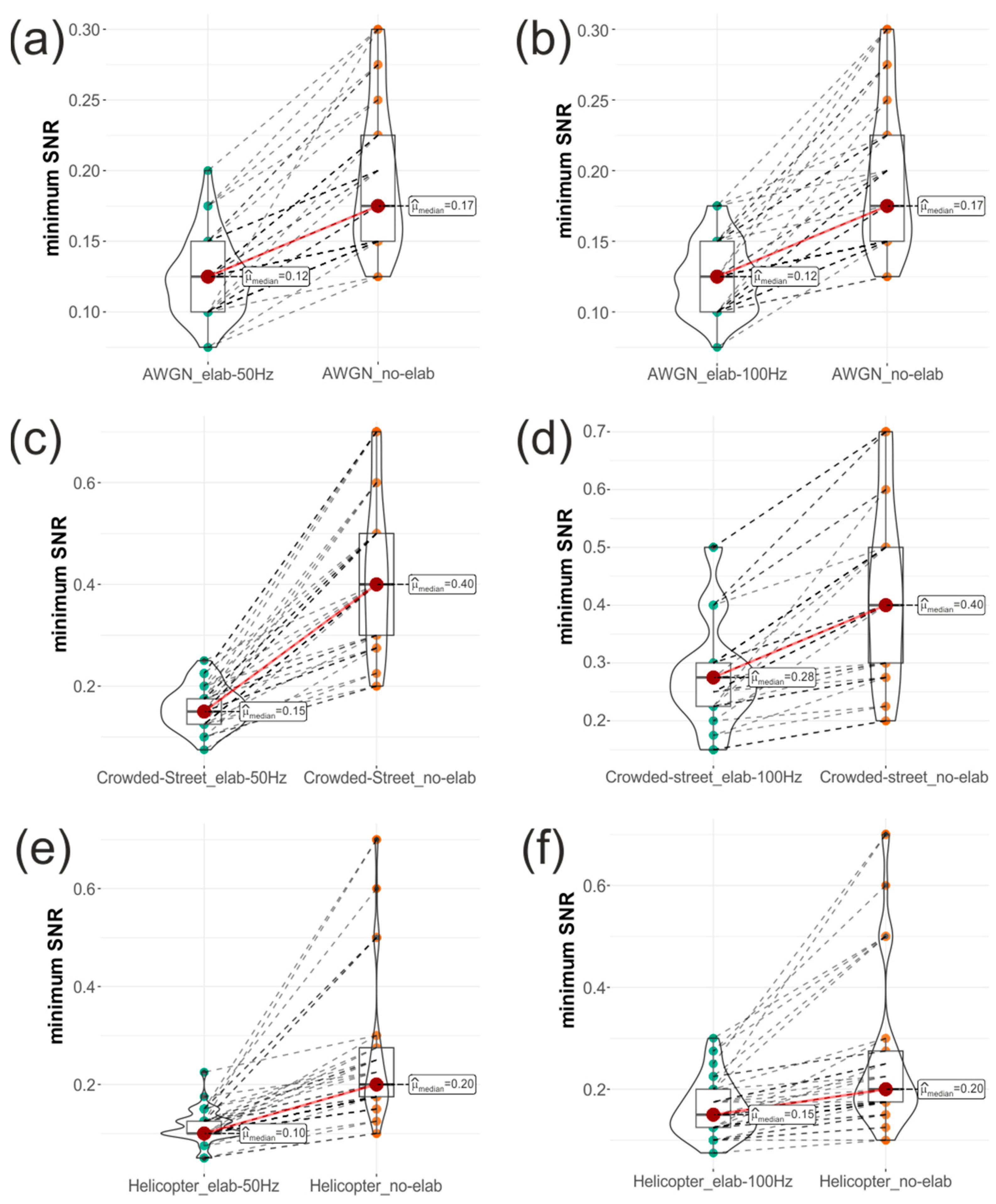
3.2. Auscultation Tests Results
4. Discussion
5. Conclusions
Author Contributions
Funding
Data Availability Statement
Conflicts of Interest
References
- Thomas, S.L.; Heaton, J.; Makaryus, A.N. Physiology, Cardiovascular Murmurs. In StatPearls; StatPearls Publishing: Treasure Island, FL, USA, 2022. [Google Scholar]
- Prakash, R.; Moorthy, K.; Aronow, W.S. First heart sound: A phono-echocardiographic correlation with mitral, tricuspid, and aortic valvular events. Catheter. Cardiovasc. Diagn. 1976, 2, 381–387. [Google Scholar] [CrossRef]
- Mehta, N.J.; Khan, I.A. Third heart sound: Genesis and clinical importance. Int. J. Cardiol. 2004, 97, 183–186. [Google Scholar] [CrossRef]
- Pelech, A.N. The physiology of cardiac auscultation. Pediatr. Clin. N. Am. 2004, 51, 1515–1535. [Google Scholar] [CrossRef] [PubMed]
- Rushmer, R.F. Cardiovascular Dynamics, 4th ed.; W.B. Saunders: Philadelphia, PA, USA, 1976; ISBN 13:9780721678474. [Google Scholar]
- Leatham, A. Auscultation of the Heart and Phonocardiography; Churchill: Livingstone, Zambia, 1970; ISBN -10 070001490X. ISBN -13 9780700014903. [Google Scholar]
- Nowak, L.J.; Nowak, K.M. Sound differences between electronic and acoustic stethoscopes. Biomed. Eng. Online 2018, 17, 104. [Google Scholar] [CrossRef] [PubMed]
- Weiss, D.; Erie, C.; Iii, J.B.; Copt, R.; Yeaw, G.; Harpster, M.; Hughes, J.; Salem, D.N. An in vitro acoustic analysis and comparison of popular stethoscopes. Med. Devices Évid. Res. 2019, 12, 41–52. [Google Scholar] [CrossRef] [PubMed]
- Silverman, B.; Balk, M. Digital Stethoscope—Improved Auscultation at the Bedside. Am. J. Cardiol. 2019, 123, 984–985. [Google Scholar] [CrossRef] [PubMed]
- Kalinauskienė, E.; Razvadauskas, H.; Morse, D.J.; Maxey, G.E.; Naudžiūnas, A. A Comparison of Electronic and Traditional Stethoscopes in the Heart Auscultation of Obese Patients. Medicina 2019, 55, 94. [Google Scholar] [CrossRef]
- Mohamed, N.; Kim, H.-S.; Kang, K.-M.; Mohamed, M.; Kim, S.-H.; Kim, J.G. Heart and Lung Sound Measurement Using an Esophageal Stethoscope with Adaptive Noise Cancellation. Sensors 2021, 21, 6757. [Google Scholar] [CrossRef]
- WHO. World Health Statistics 2021: Monitoring Health for the SDGs, Sustainable Development Goals; WHO: Geneva, Switzerland, 2021. [Google Scholar]
- Andreozzi, E.; Gargiulo, G.D.; Esposito, D.; Bifulco, P. A Novel Broadband Forcecardiography Sensor for Simultaneous Monitoring of Respiration, Infrasonic Cardiac Vibrations and Heart Sounds. Front. Physiol. 2021, 12, 725716. [Google Scholar] [CrossRef]
- Ha, T.; Tran, J.; Liu, S.; Jang, H.; Jeong, H.; Mitbander, R.; Huh, H.; Qiu, Y.; Duong, J.; Wang, R.L.; et al. A Chest-Laminated Ultrathin and Stretchable E-Tattoo for the Measurement of Electrocardiogram, Seismocardiogram, and Cardiac Time Intervals. Adv. Sci. 2019, 6, 1900290. [Google Scholar] [CrossRef] [PubMed]
- Liu, Y.; Norton, J.J.S.; Qazi, R.; Zou, Z.; Ammann, K.R.; Liu, H.; Yan, L.; Tran, P.L.; Jang, K.-I.; Lee, J.W.; et al. Epidermal mechano-acoustic sensing electronics for cardiovascular diagnostics and human-machine interfaces. Sci. Adv. 2016, 2, e1601185. [Google Scholar] [CrossRef]
- Gupta, P.; Moghimi, M.J.; Jeong, Y.; Gupta, D.; Inan, O.T.; Ayazi, F. Precision wearable accelerometer contact microphones for longitudinal monitoring of mechano-acoustic cardiopulmonary signals. NPJ Digit. Med. 2020, 3, 19. [Google Scholar] [CrossRef]
- Andreozzi, E.; Gargiulo, G.D.; Fratini, A.; Esposito, D.; Bifulco, P. A Contactless Sensor for Pacemaker Pulse Detection: Design Hints and Performance Assessment. Sensors 2018, 18, 2715. [Google Scholar] [CrossRef]
- Liu, F.; Wang, Y.T.; Wang, Y.X. Research and Implementation of Heart Sound Denoising. Phys. Procedia 2012, 25, 777–785. [Google Scholar] [CrossRef]
- Vikhe, P.S.; Nehe, N.S.; Thool, V.R. Heart Sound Abnormality Detection Using Short Time Fourier Transform and Con-tinuous Wavelet Transform. In Proceedings of the 2009 Second International Conference on Emerging Trends in Engineering & Technology, Nagpur, India, 16–18 December 2009; pp. 50–54. [Google Scholar]
- Zia, M.K.; Griffel, B.; Semmlow, J.L. Robust detection of background noise in phonocardiograms. In Proceedings of the 2011 1st Middle East Conference on Biomedical Engineering, Sharjah, United Arab Emirates, 21–24 February 2011; pp. 130–133. [Google Scholar] [CrossRef]
- Tang, H.; Li, T.; Park, Y.; Qiu, T. Separation of Heart Sound Signal from Noise in Joint Cycle Frequency–Time–Frequency Domains Based on Fuzzy Detection. IEEE Trans. Biomed. Eng. 2010, 57, 2438–2447. [Google Scholar] [CrossRef] [PubMed]
- Gradolewski, D.; Redlarski, G. Wavelet-based denoising method for real phonocardiography signal recorded by mobile devices in noisy environment. Comput. Biol. Med. 2014, 52, 119–129. [Google Scholar] [CrossRef] [PubMed]
- Yoganathan, A.P.; Gupta, R.; Udwadia, F.E.; Miller, J.W.; Corcoran, W.H.; Sarma, R.; Johnson, J.L.; Bing, R.J. Use of the fast fourier transform for frequency analysis of the first heart sound in normal man. Med. Biol. Eng. Comput. 1976, 14, 69–73. [Google Scholar] [CrossRef]
- Debbal, S.; Bereksi-Reguig, F. Computerized heart sounds analysis. Comput. Biol. Med. 2008, 38, 263–280. [Google Scholar] [CrossRef]
- Naseri, H.; Homaeinezhad, M.; Pourkhajeh, H. Noise/spike detection in phonocardiogram signal as a cyclic random process with non-stationary period interval. Comput. Biol. Med. 2013, 43, 1205–1213. [Google Scholar] [CrossRef] [PubMed]
- Rouis, M.; Sbaa, S.; Benhassine, N.E. The effectiveness of the choice of criteria on the stationary and non-stationary noise removal in the phonocardiogram (PCG) signal using discrete wavelet transform. Biomed. Eng./Biomed. Tech. 2020, 65, 353–366. [Google Scholar] [CrossRef]
- Wang, F.; Ji, Z. Application of the Dual-tree Complex Wavelet Transform in Biomedical Signal Denoising. Bio-Medical Mater. Eng. 2014, 24, 109–115. [Google Scholar] [CrossRef] [PubMed]
- Ali, M.N.; El-Dahshan, E.-S.A.; Yahia, A.H. Denoising of Heart Sound Signals Using Discrete Wavelet Transform. Circuits Syst. Signal Process. 2017, 36, 4482–4497. [Google Scholar] [CrossRef]
- Singh, B.N.; Tiwari, A.K. Optimal selection of wavelet basis function applied to ECG signal denoising. Digit. Signal Process. 2006, 16, 275–287. [Google Scholar] [CrossRef]
- Debbal, S.M.; Bereksi-Reguig, F. Time-frequency analysis of the first and the second heart beat sounds. Appl. Math. Comput. 2007, 184, 1041–1052. [Google Scholar]
- Gradolewski, D.; Redlarski, G. The use of wavelet analysis to denoising of electrocardiography signal. In Proceedings of the XV International PhD Workshop, Wisła, Poland, 19–22 October 2013; pp. 456–461. [Google Scholar]
- Debbal, S.; Bereksi-Reguig, F. Analysis of the second heart sound using continuous wavelet transform. J. Med. Eng. Technol. 2009, 28, 151–156. [Google Scholar] [CrossRef]
- Messer, S.R.; Agzarian, J.; Abbott, D. Optimal wavelet denoising for phonocardiograms. Microelectron. J. 2001, 32, 931–941. [Google Scholar] [CrossRef]
- Jain, P.K.; Tiwari, A.K. An adaptive thresholding method for the wavelet based denoising of phonocardiogram signal. Biomed. Signal Process. Control. 2017, 38, 388–399. [Google Scholar] [CrossRef]
- Zhou, K.L.; Liu, Y.Y. Heart Sound Denoising of New Threshold Wavelet Transform. Comput. Eng. Des. 2020, 41, 2476–2481. [Google Scholar]
- Li, S.; Li, F.; Tang, S.; Xiong, W. A Review of Computer-Aided Heart Sound Detection Techniques. BioMed Res. Int. 2020, 2020, 1–10. [Google Scholar] [CrossRef]
- Xie-Feng, C.; Bin, J.; He, Y.; YuFeng, G.; ShaoBai, Z. A new method of heart sound signal analysis based on independent function element. AIP Adv. 2014, 4, 097131. [Google Scholar] [CrossRef]
- Zhao, X.; Ye, B. Convolution wavelet packet transform and its applications to signal processing. Digit. Signal Process. 2010, 20, 1352–1364. [Google Scholar] [CrossRef]
- Safara, F.; Doraisamy, S.; Azman, A.; Jantan, A.; Abdullah Ramaiah, A.R. Multi-level basis selection of wavelet packet decom-position tree for heart sound classification. Comput. Biol. Med. 2013, 43, 1407–1408. [Google Scholar] [CrossRef] [PubMed]
- Huang, N.E.; Shen, Z.; Long, S.R.; Wu, M.C.; Shih, H.H.; Zheng, Q.; Yen, N.-C.; Tung, C.C.; Liu, H.H. The empirical mode decomposition and the Hilbert spectrum for nonlinear and non-stationary time series analysis. Proc. R. Soc. Lond. Ser. A Math. Phys. Eng. Sci. 1998, 454, 903–995. [Google Scholar] [CrossRef]
- Salman, A.H.; Ahmadi, N.; Mengko, R.; Langi, A.Z.R.; Mengko, T.L.R. Empirical Mode Decomposition (EMD) Based Denoising Method for Heart Sound Signal and Its Performance Analysis. Int. J. Electr. Comput. Eng. 2016, 6, 2197–2204. [Google Scholar]
- Gao, Y.; Ge, G.; Sheng, Z.; Sang, E. Analysis and Solution to the Mode Mixing Phenomenon in EMD. In Proceedings of the 2008 Congress on Image and Signal Processing, Sanya, China, 27–30 May 2008; pp. 223–227. [Google Scholar] [CrossRef]
- Gaci, S. A New Ensemble Empirical Mode Decomposition (EEMD) Denoising Method for Seismic Signals. Energy Procedia 2016, 97, 84–91. [Google Scholar] [CrossRef]
- Wu, Z.H.; Huang, N.E. Ensemble empirical mode decomposition: A noise-assisted data analysis Method. AADA Adv. Adapt. Data Anal. 2009, 1, 1–4. [Google Scholar] [CrossRef]
- Yeh, J.-R.; Shieh, J.-S.; Huang, N.E. Complementary ensemble empirical mode decomposition: A novel noise enhanced data analysis method. Adv. Adapt. Data Anal. 2010, 2, 135–156. [Google Scholar] [CrossRef]
- Dong, L.C.; Guo, X.M.; Zheng, Y.N. Wavelet Packet De-Noising Algorithm for Heart Sound Signals Based on CEEMD. J. Vib. Shock. 2019, 38, 192–198+222. [Google Scholar]
- Dragomiretskiy, K.; Zosso, D. Variational Mode Decomposition. IEEE Trans. Signal Process. 2014, 62, 531–544. [Google Scholar] [CrossRef]
- Banerjee, S.; Mishra, M.; Mukherjee, A. Segmentation and detection of first and second heart sounds (Si and S2) using variational mode decomposition. In Proceedings of the 2016 IEEE EMBS Conference on Biomedical Engineering and Sciences (IECBES), Kuala Lumpur, Malaysia, 4–8 December 2016; pp. 565–570. [Google Scholar] [CrossRef]
- Liu, Q.; Xu, Y.; Zhang, L.; Liang, C. Research on Heart Sound Signal Denoising Algorithm Based on Variational Mode Decomposition and Wavelet Threshold. J. Comput. Commun. 2021, 9, 110–121. [Google Scholar] [CrossRef]
- Rudin, L.I.; Osher, S.; Fatemi, E. Nonlinear total variation based noise removal algorithms. Phys. D Nonlinear Phenom. 1992, 60, 259–268. [Google Scholar] [CrossRef]
- Varghees, V.N.; Ramachandran, K. A novel heart sound activity detection framework for automated heart sound analysis. Biomed. Signal Process. Control. 2014, 13, 174–188. [Google Scholar] [CrossRef]
- Haykin, S. Unsupervised Adaptive Filtering: Volume I Blind Source Separation; Wiley: New York, NY, USA, 2000. [Google Scholar]
- Zheng, H.; Wang, H.; Wang, L.Y.; Yin, G.G. Cyclic system reconfiguration and time-split signal separation with applications to lung sound pattern analysis. IEEE Trans. Signal Process. 2007, 55, 2897–2913. [Google Scholar] [CrossRef]
- Shah, G.; Koch, P.; Papadias, C.B. On the Blind Recovery of Cardiac and Respiratory Sounds. IEEE J. Biomed. Health Inform. 2014, 19, 151–157. [Google Scholar] [CrossRef]
- Emmanouilidou, D.; McCollum, E.D.; Park, D.E.; Elhilali, M. Adaptive Noise Suppression of Pediatric Lung Auscultations with Real Applications to Noisy Clinical Settings in Developing Countries. IEEE Trans. Biomed. Eng. 2015, 62, 2279–2288. [Google Scholar] [CrossRef]
- Khan, A.K.; Onoue, T.; Hashiodani, K.; Fukumizu, Y.; Yamauchi, H. Signal and noise separation in medical diagnostic system based on independent component analysis. In Proceedings of the 2010 IEEE Asia Pacific Conference on Circuits and Systems, Kuala Lumpur, Malaysia, 6–9 December 2010; pp. 812–815. [Google Scholar] [CrossRef]
- Hunt, R.C.; Bryan, D.M.; Brinkley, V.S.; Whitley, T.W.; Benson, N.H. Inability to assess breath sounds during air medical transport by helicopter. JAMA 1991, 265, 1982–1984. [Google Scholar] [CrossRef]
- Nelson, G.; Rajamani, R.; Erdman, A. Noise control challenges for auscultation on medical evacuation helicopters. Appl. Acoust. 2014, 80, 68–78. [Google Scholar] [CrossRef]
- Tourtier, J.P.; Fontaine, E.; Coste, S.; Ramsang, S.; Schiano, P.; Viaggi, M.; Libert, N.; Durand, X.; Chargari, C.; Borne, M. In flight auscultation: Comparison of electronic and conventional stethoscopes. Am. J. Emerg. Med. 2011, 29, 932–935. [Google Scholar] [CrossRef] [PubMed]
- Fontaine, E.; Coste, S.; Poyat, C.; Klein, C.; Lefort, H.; Leclerc, T.; Dubourdieu, S.; Briche, F.; Jost, D.; Maurin, O.; et al. In-flight auscultation during medical air evacuation: Comparison between traditional and amplified stethoscopes. Air Med. J. 2014, 33, 283–285. [Google Scholar] [CrossRef] [PubMed]
- Brown, L.H.; E Gough, J.; Bryan-Berg, D.M.; Hunt, R.C. Assessment of breath sounds during ambulance transport. Ann. Emerg. Med. 1997, 29, 228–231. [Google Scholar] [CrossRef]
- Zun, L.S.; Downey, L. The Effect of Noise in the Emergency Department. Acad. Emerg. Med. 2005, 12, 663–666. [Google Scholar] [CrossRef] [PubMed]
- Mallinson, T. Prehospital cardiac auscultation: Friend or foe? J. Paramed. Pract. 2010, 2, 256–259. [Google Scholar] [CrossRef]
- McLane, I.; Emmanouilidou, D.; E West, J.; Elhilali, M. Design and Comparative Performance of a Robust Lung Auscultation System for Noisy Clinical Settings. IEEE J. Biomed. Health Inform. 2021, 25, 2583–2594. [Google Scholar] [CrossRef] [PubMed]
- Holloway, G.A., Jr.; Watkins, D. An electronic frequency shifting stethoscope for heart sounds. J. Bioeng. 1978, 2, 59–64. [Google Scholar] [PubMed]
- Jung, D.K. Reinforcing Stethoscope Sound using Spectral Shift. J. Sens. Sci. Technol. 2021, 30, 47–50. [Google Scholar] [CrossRef]
- Aumann, H.M.; Emanetoglu, N.W. Stethoscope with digital frequency translation for improved audibility. Healthc. Technol. Lett. 2019, 6, 143–146. [Google Scholar] [CrossRef]
- Houtsma, A.J.M.; Curry, I.P.; Sewell, J.M.; Bernard, W.N. Auscultation in high-noise environments using hybrid electromechanical and ultrasound-Doppler techniques. J. Acoust. Soc. Am. 2006, 120, 3361. [Google Scholar] [CrossRef]
- Gaydos, S. Clinical auscultation in noisy environments. J. Emerg. Med. 2012, 43, 492–493. [Google Scholar] [CrossRef]
- Strollo, A.G.M.; De Caro, D. Direct Digital Frequency Synthesizers exploiting Piecewise Linear Chebyshev Approximation. Microelectron. J. 2003, 34, 1099–1106. [Google Scholar] [CrossRef]
- Classification of Heart Sound Recordings: The PhysioNet/Computing in Cardiology Challenge. Available online: https://physionet.org/content/challenge-2016/1.0.0/ (accessed on 10 February 2021).
- Available online: https://pixabay.com/it/sound-effects/crowded-avenue-people-talking-vendors-shouting-musicians-playing-part-1-7099/ (accessed on 15 July 2022).
- Available online: https://pixabay.com/it/sound-effects/helicopter-8030/ (accessed on 15 July 2022).
- TMS320C6711D, C6712D, C6713B Power Consumption Summary; Texas Instruments Application Report SPRA889A. 2005.


| Technique | Low-Sideband Noise Power/Output Power |
|---|---|
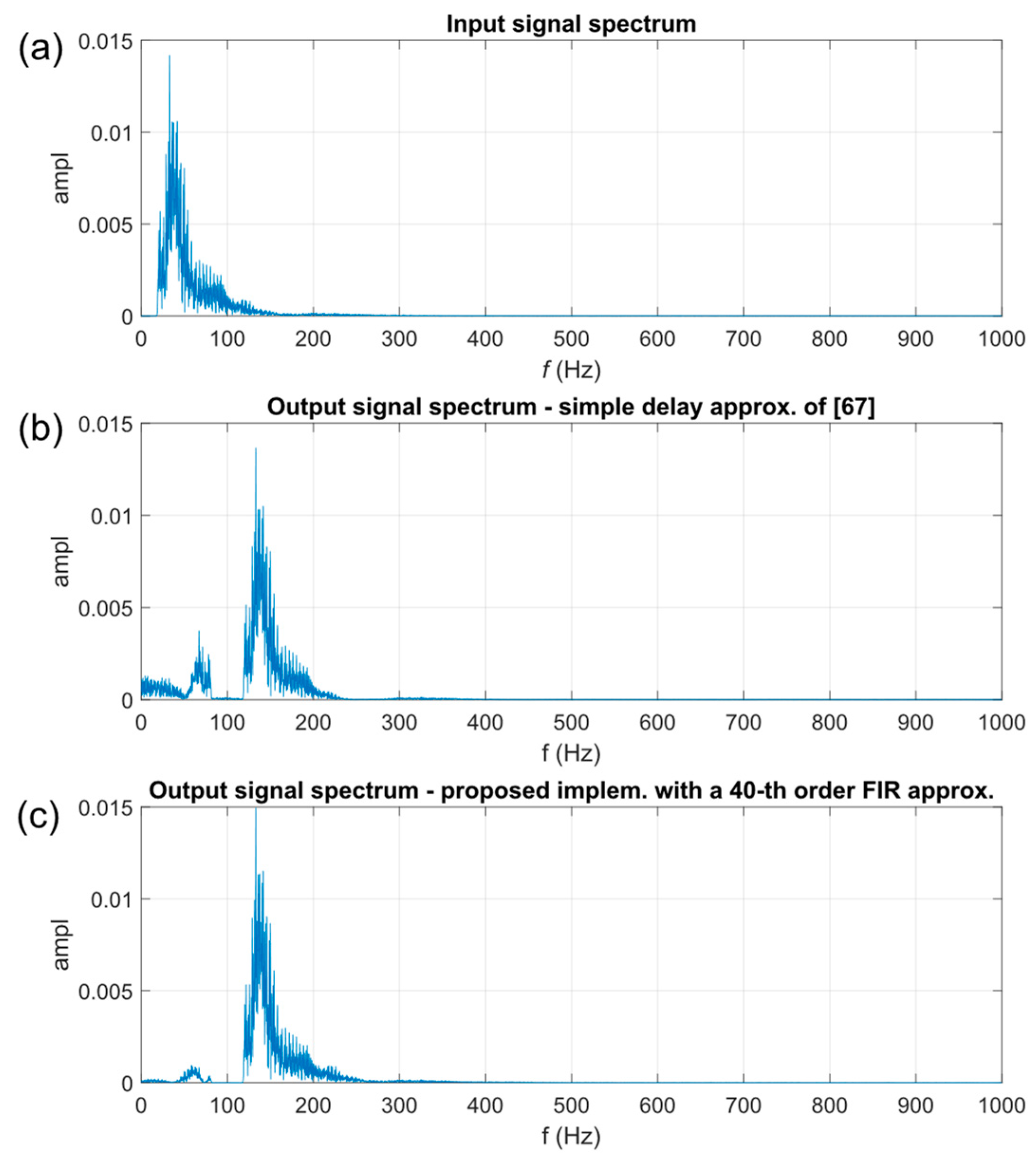
| Simple delay approx. [67] | −11.9 dB |
| Proposed with 20-th order FIR filter | −21.2 dB |
| Proposed with 40-th order FIR filter | −23.3 dB |
| Proposed with 60-th order FIR filter | −30.3 dB |
| Proposed with 80-th order FIR filter | −37.7 dB |
| Proposed with 100-th order FIR filter | −42.9 dB |
| Number of Sub-Intervals (2H) | Piecewise Linear Approx | Piecewise Quadratic Approx |
|---|---|---|
| εalg/LSBy | εalg/LSBy | |
| 4 | 78.893 | 1.291 |
| 8 | 19.735 | 0.161 |
| 16 | 4.935 | 0.020 |
| 32 | 1.234 | 2.52 × 10⁻³ |
| 64 | 0.308 | 3.15 × 10⁻⁴ |
| 128 | 0.077 | 3.94 × 10⁻⁵ |
| Maximum Absolute Errors Normalized to LSBy | ||||||||||
|---|---|---|---|---|---|---|---|---|---|---|
| Piecewise Approx. (εalg) | a0 i Coeff. | a1 i Coeff. | a2 i Coeff. | z Signal | z2 Signal | Inputs of the Adder in Figure 6 | Adder Output in Figure 6 | Total Error | Total Error (Simulat.) | |
| LSB Reduction Method | - | Rounding | Rounding | Rounding | Rounding | Trunc. | Trunc. | Rounding | - | - |
| Piecewise linear technique | 0.077 | 7.63 × 10⁻⁶ | 0.002 | - | 0.002 | - | 1.53 × 10⁻⁵ | 0.500 | 0.581 | 0.576 |
| Piecewise quadratic technique | 0.161 | 7.63 × 10⁻⁶ | 0.031 | 5.96 × 10⁻⁸ | 0.025 | 0.005 | 3.05 × 10⁻⁵ | 0.500 | 0.722 | 0.684 |
| Sin/Cos Computation Technique | LUT Storage Tech. | LUT Size (Bytes) | Code Size (Bytes) | Total Memory Size (Bytes) | Percentage BSS Section Occupation | Execution Time (Clock Cycles) |
|---|---|---|---|---|---|---|
| Piecewise Lineax Approx. | far alloc. | 1536 | 224 | 1760 | - | 25.0 |
| Piecewise Lineax Approx. | near alloc. | 1536 | 224 | 1760 | 4.7% | 19.0 |
| Piecewise Quadratic Approx. | near alloc. | 128 | 256 | 384 | 0.4% | 21.0 |
| Library functions—Single-Precision | - | - | 928 | 928 | - | 177.0 |
| Library functions—Double-Precision | - | - | 1120 | 1120 | - | 346.5 |
| Sin/Cos Computation Technique | LUT Storage Tech. | Memory Size (Bytes) | Execution Time (Clock Cycles) | |||||||||
|---|---|---|---|---|---|---|---|---|---|---|---|---|
| DDFS LUT | FIR LUT | DDFS Code | FIR Code | Code Other | Total | DDFS | FIR Sum-of-Prod. | FIR Buffer Update | Other | Total | ||
| Piecewise Lineax Approx. | far alloc. | 1536 | 84 | 224 | 64 | 640 | 2548 | 25.0 | 28.0 | 46.0 | 29.0 | 128.0 |
| Piecewise Lineax Approx. | near alloc. | 1536 | 84 | 224 | 64 | 640 | 2548 | 19.0 | 28.0 | 46.0 | 29.0 | 122.0 |
| Piecewise Quadratic Approx. | near alloc. | 128 | 84 | 256 | 64 | 640 | 1172 | 21.0 | 28.0 | 46.0 | 29.0 | 124.0 |
| Library functions—Single-Precision | - | - | 84 | 928 | 64 | 640 | 1716 | 177.0 | 28.0 | 46.0 | 29.0 | 280.0 |
| Library functions—Double-Precision | - | - | 84 | 1120 | 64 | 640 | 1908 | 342.0 | 28.0 | 46.0 | 29.0 | 445.0 |
| Sin/Cos Computation Technique | LUT Storage Tech. | Execution Time (Clock Cycles) | |||
|---|---|---|---|---|---|
| Core Elaboration (Frequency Shift) | Down/Up Sampling | ISRs | Total | ||
| Piecewise Lineax Approx. | far alloc. | 128.2 | 221.0 | 63.0 | 412.2 |
| Piecewise Lineax Approx. | near alloc. | 122.2 | 215.0 | 62.3 | 399.5 |
| Piecewise Quadratic Approx. | near alloc. | 124.1 | 218.2 | 62.3 | 404.7 |
| Library functions—Single-Precision | - | 285.2 | 214.1 | 62.6 | 561.9 |
| Library functions—Double-Precision | - | 510.2 | 228.2 | 69.4 | 807.8 |
| Sin/Cos Computation Technique | LUT Storage Tech. | Code Size (Bytes) | Data Size (Bytes) | ||||||
|---|---|---|---|---|---|---|---|---|---|
| Core Elaboration (Frequency Shift) | Down/Up Sampling | ISRs | Total | Core Elaboration (Frequency Shift) | Down/Up Sampling | ISRs | Total | ||
| Piecewise Lineax Approx. | far alloc. | 928 | 1280 | 1184 | 3392 | 1620 | 280 | 70 | 1970 |
| Piecewise Lineax Approx. | near alloc. | 928 | 1280 | 1184 | 3392 | 1620 | 280 | 70 | 1970 |
| Piecewise Quadratic Approx. | near alloc. | 960 | 1280 | 1184 | 3424 | 212 | 280 | 70 | 562 |
| Library functions—Single-Precision | - | 1632 | 1280 | 1184 | 4096 | 84 | 280 | 70 | 434 |
| Library functions—Double-Precision | - | 1824 | 1280 | 1184 | 4288 | 84 | 280 | 70 | 434 |
| Sin/Cos Computation Technique | LUT Storage Tech. | Minimum DSP Clock Freq. (MHz) | Power estimation | ||||
|---|---|---|---|---|---|---|---|
| Avg. Istr. Executed per Clock Cycle | DSP Core Utilization (%) | Dynamic Power (mW) | |||||
| Activity Power | Clock Tree | Total Power | |||||
| Piecewise Lineax Approx. | far alloc. | 0.824 | 4.02 | 50.2% | 0.58 | 1.76 | 2.35 |
| Piecewise Lineax Approx. | near alloc. | 0.799 | 4.09 | 51.1% | 0.57 | 1.71 | 2.28 |
| Piecewise Quadratic Approx. | near alloc. | 0.809 | 4.11 | 51.4% | 0.58 | 1.73 | 2.31 |
| Library functions—Single-Precision | - | 1.124 | 2.95 | 36.8% | 0.61 | 2.40 | 3.01 |
| Library functions—Double-Precision | - | 1.616 | 2.20 | 27.5% | 0.69 | 3.46 | 4.14 |
| Noise Source | Processing | Min | 1st Quartile | Median | Mean | 3rd Quartile | Max | SD |
|---|---|---|---|---|---|---|---|---|
| AWGN | no_elab | 0.125 | 0.150 | 0.175 | 0.195 | 0.225 | 0.300 | 0.05038 |
| elab_50 | 0.075 | 0.100 | 0.125 | 0.124 | 0.150 | 0.200 | 0.02766 | |
| elab_100 | 0.075 | 0.100 | 0.125 | 0.124 | 0.150 | 0.175 | 0.02468 | |
| CROWDED STREET | no_elab | 0.200 | 0.300 | 0.400 | 0.423 | 0.500 | 0.700 | 0.15236 |
| elab_50 | 0.075 | 0.125 | 0.150 | 0.158 | 0.175 | 0.250 | 0.04087 | |
| elab_100 | 0.150 | 0.225 | 0.275 | 0.282 | 0.300 | 0.500 | 0.09087 | |
| HELICOPTER | no_elab | 0.100 | 0.175 | 0.200 | 0.259 | 0.275 | 0.700 | 0.15550 |
| elab_50 | 0.050 | 0.100 | 0.100 | 0.114 | 0.125 | 0.225 | 0.03309 | |
| elab_100 | 0.075 | 0.125 | 0.150 | 0.161 | 0.200 | 0.300 | 0.05392 |
| Noise Source | Comparison | W | z-val | p-Value | rrb | # Pairs |
|---|---|---|---|---|---|---|
| AWGN | elab_50 Hz vs. no_elab | 861 | 5.61 | 1.005 × 10⁻⁸ | 1.00 | 41 |
| elab_100 Hz vs. no_elab | 861 | 5.60 | 1.057 × 10⁻⁸ | 1.00 | 41 | |
| CROWDED STREET | elab_50 Hz vs. no_elab | 861 | 5.58 | 1.212 × 10⁻⁸ | 1.00 | 41 |
| elab_100 Hz vs. no_elab | 861 | 5.59 | 1.107 × 10⁻⁸ | 1.00 | 41 | |
| HELICOPTER | elab_50 Hz vs. no_elab | 861 | 5.60 | 1.066 × 10⁻⁸ | 1.00 | 41 |
| elab_100 Hz vs. no_elab | 780 | 5.47 | 2.210 × 10⁻⁸ | 1.00 | 39 |
Disclaimer/Publisher’s Note: The statements, opinions and data contained in all publications are solely those of the individual author(s) and contributor(s) and not of MDPI and/or the editor(s). MDPI and/or the editor(s) disclaim responsibility for any injury to people or property resulting from any ideas, methods, instructions or products referred to in the content. |
© 2023 by the authors. Licensee MDPI, Basel, Switzerland. This article is an open access article distributed under the terms and conditions of the Creative Commons Attribution (CC BY) license (https://creativecommons.org/licenses/by/4.0/).
Share and Cite
Muto, V.; Andreozzi, E.; Cappelli, C.; Centracchio, J.; Di Meo, G.; Esposito, D.; Bifulco, P.; De Caro, D. Real-Time Implementation of a Frequency Shifter for Enhancement of Heart Sounds Perception on VLIW DSP Platform. Electronics 2023, 12, 4359. https://doi.org/10.3390/electronics12204359
Muto V, Andreozzi E, Cappelli C, Centracchio J, Di Meo G, Esposito D, Bifulco P, De Caro D. Real-Time Implementation of a Frequency Shifter for Enhancement of Heart Sounds Perception on VLIW DSP Platform. Electronics. 2023; 12(20):4359. https://doi.org/10.3390/electronics12204359
Chicago/Turabian StyleMuto, Vincenzo, Emilio Andreozzi, Carmela Cappelli, Jessica Centracchio, Gennaro Di Meo, Daniele Esposito, Paolo Bifulco, and Davide De Caro. 2023. "Real-Time Implementation of a Frequency Shifter for Enhancement of Heart Sounds Perception on VLIW DSP Platform" Electronics 12, no. 20: 4359. https://doi.org/10.3390/electronics12204359
APA StyleMuto, V., Andreozzi, E., Cappelli, C., Centracchio, J., Di Meo, G., Esposito, D., Bifulco, P., & De Caro, D. (2023). Real-Time Implementation of a Frequency Shifter for Enhancement of Heart Sounds Perception on VLIW DSP Platform. Electronics, 12(20), 4359. https://doi.org/10.3390/electronics12204359