Figure 1.
Analog bell-shaped classifier with classes, clusters/centroids, and features. This is a conceptual design describing the general methodology.
Figure 1.
Analog bell-shaped classifier with classes, clusters/centroids, and features. This is a conceptual design describing the general methodology.
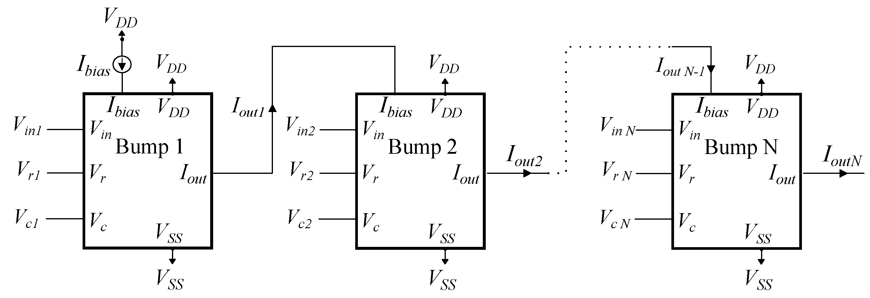
Figure 2.
By arranging a series of N basic bump circuits in sequence, the final output of this arrangement provides the behavior of an N-dimensional Gaussian function. The individual parameters (, , ) for each bump circuit are adjusted independently.
Figure 2.
By arranging a series of N basic bump circuits in sequence, the final output of this arrangement provides the behavior of an N-dimensional Gaussian function. The individual parameters (, , ) for each bump circuit are adjusted independently.
Figure 3.
The utilized Gaussian function circuit is presented. The output current resembles a Gaussian function controlled by the input voltage . The parameter voltages , and the bias current control the Gaussian function’s mean value, variance, and peak value, respectively.
Figure 3.
The utilized Gaussian function circuit is presented. The output current resembles a Gaussian function controlled by the input voltage . The parameter voltages , and the bias current control the Gaussian function’s mean value, variance, and peak value, respectively.
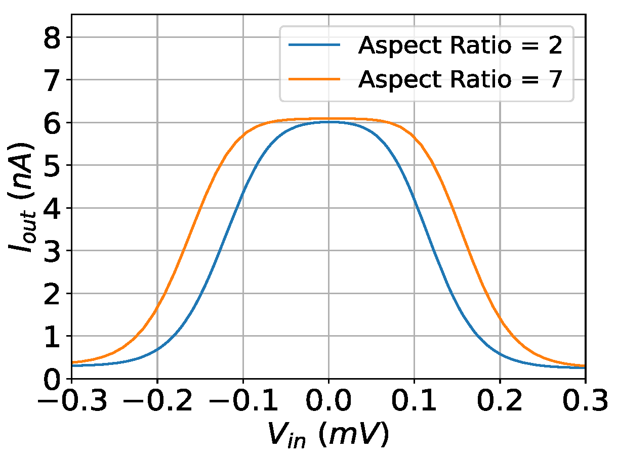
Figure 4.
The output current of the implemented bump circuit with respect to the aspect ratio of the input differential pair transistors. The simulation was conducted under V, mV, and nA.
Figure 4.
The output current of the implemented bump circuit with respect to the aspect ratio of the input differential pair transistors. The simulation was conducted under V, mV, and nA.
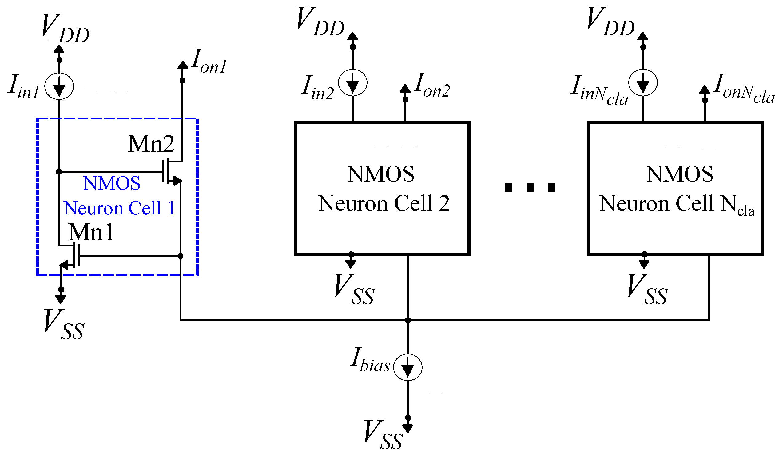
Figure 5.
A -neuron standard Lazzaro NMOS Winner-Take-All (WTA) circuit.
Figure 5.
A -neuron standard Lazzaro NMOS Winner-Take-All (WTA) circuit.
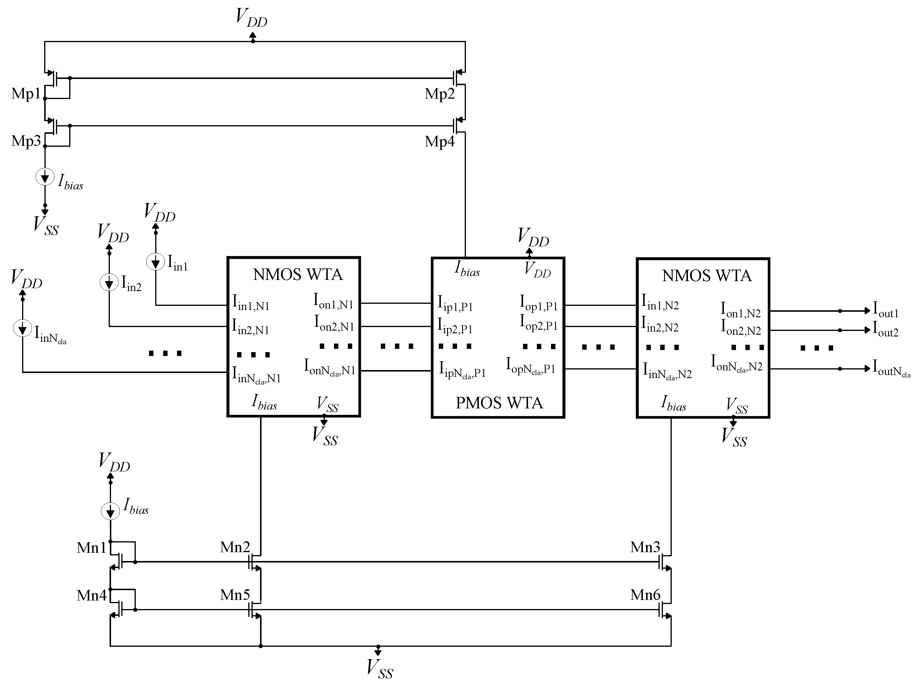
Figure 6.
A cascaded NMOS-PMOS-NMOS WTA circuit. It is utilized to improve the performance of the standard WTA circuit.
Figure 6.
A cascaded NMOS-PMOS-NMOS WTA circuit. It is utilized to improve the performance of the standard WTA circuit.
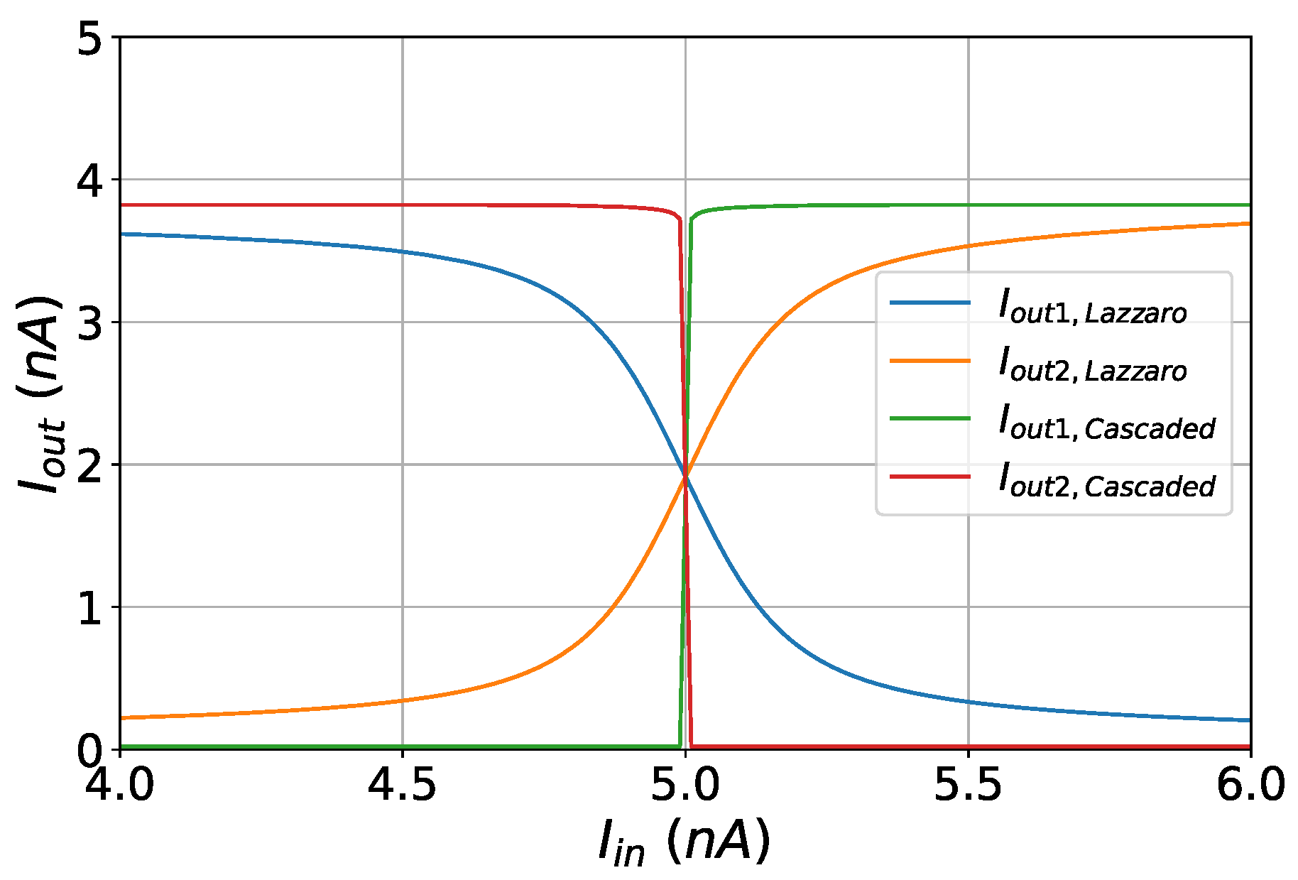
Figure 7.
Decision boundaries of the standard and the cascaded WTA circuit.
Figure 7.
Decision boundaries of the standard and the cascaded WTA circuit.
Figure 8.
Layout related to the general design methodology. It combines all the implemented CLFs and extra switches in order to select the appropriate one.
Figure 8.
Layout related to the general design methodology. It combines all the implemented CLFs and extra switches in order to select the appropriate one.
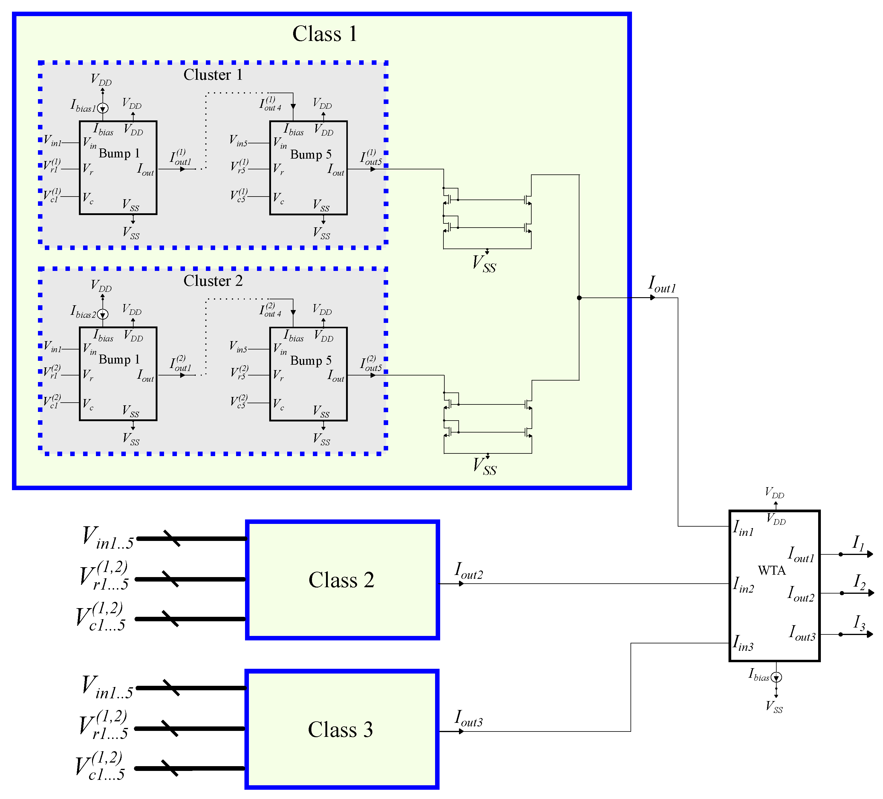
Figure 9.
An analog GMM-based classifier comprises 3 classes, 2 clusters per class, and 5 input dimensions.
Figure 9.
An analog GMM-based classifier comprises 3 classes, 2 clusters per class, and 5 input dimensions.
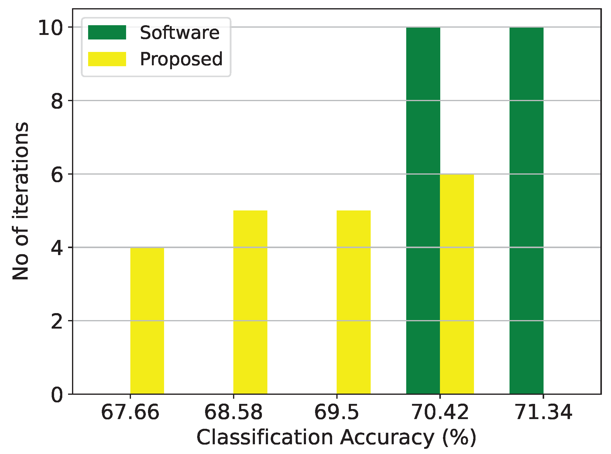
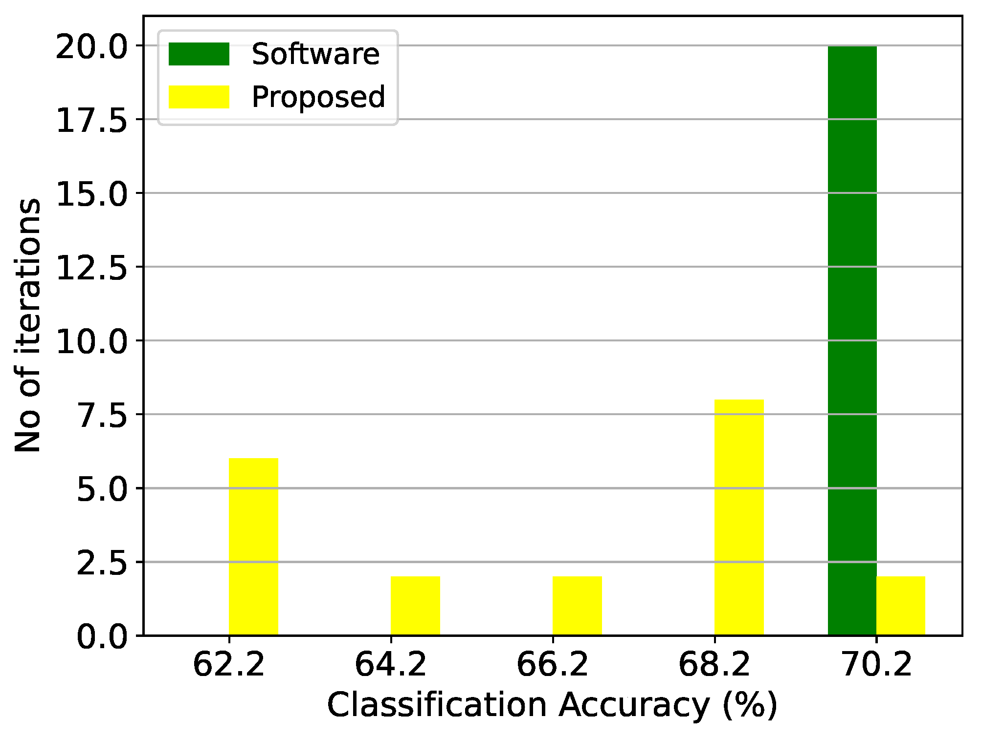
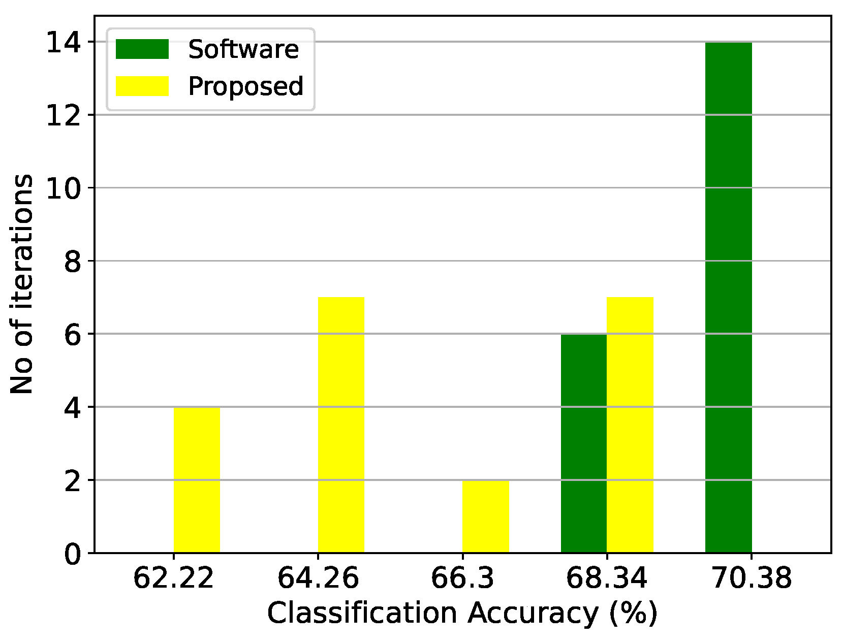
Figure 10.
Classification results of the GMM architecture and the equivalent software model on the thyroid disease detection dataset over 20 iterations.
Figure 10.
Classification results of the GMM architecture and the equivalent software model on the thyroid disease detection dataset over 20 iterations.
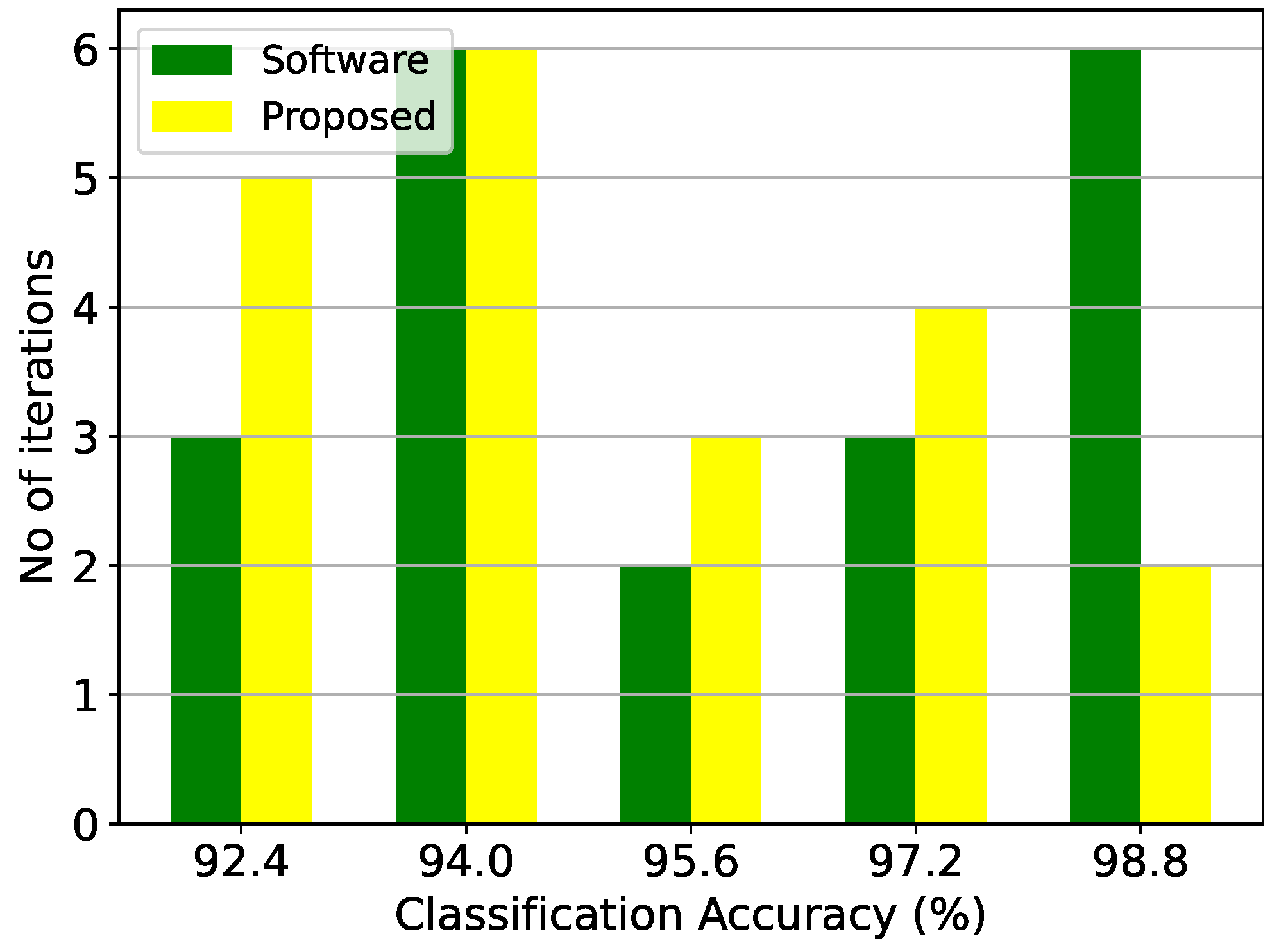
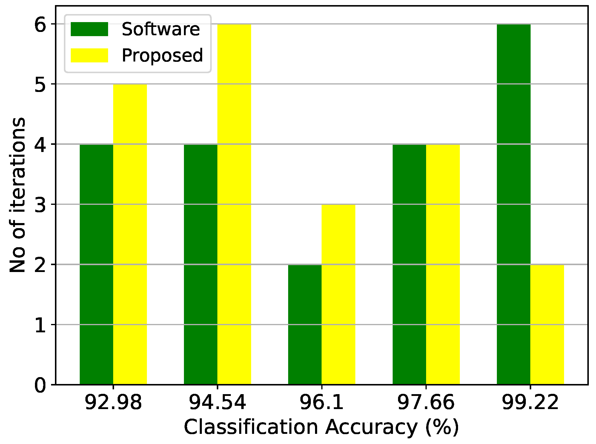
Figure 11.
Classification results of the GMM architecture and the equivalent software model on the epileptic seizure prediction dataset over 20 iterations.
Figure 11.
Classification results of the GMM architecture and the equivalent software model on the epileptic seizure prediction dataset over 20 iterations.
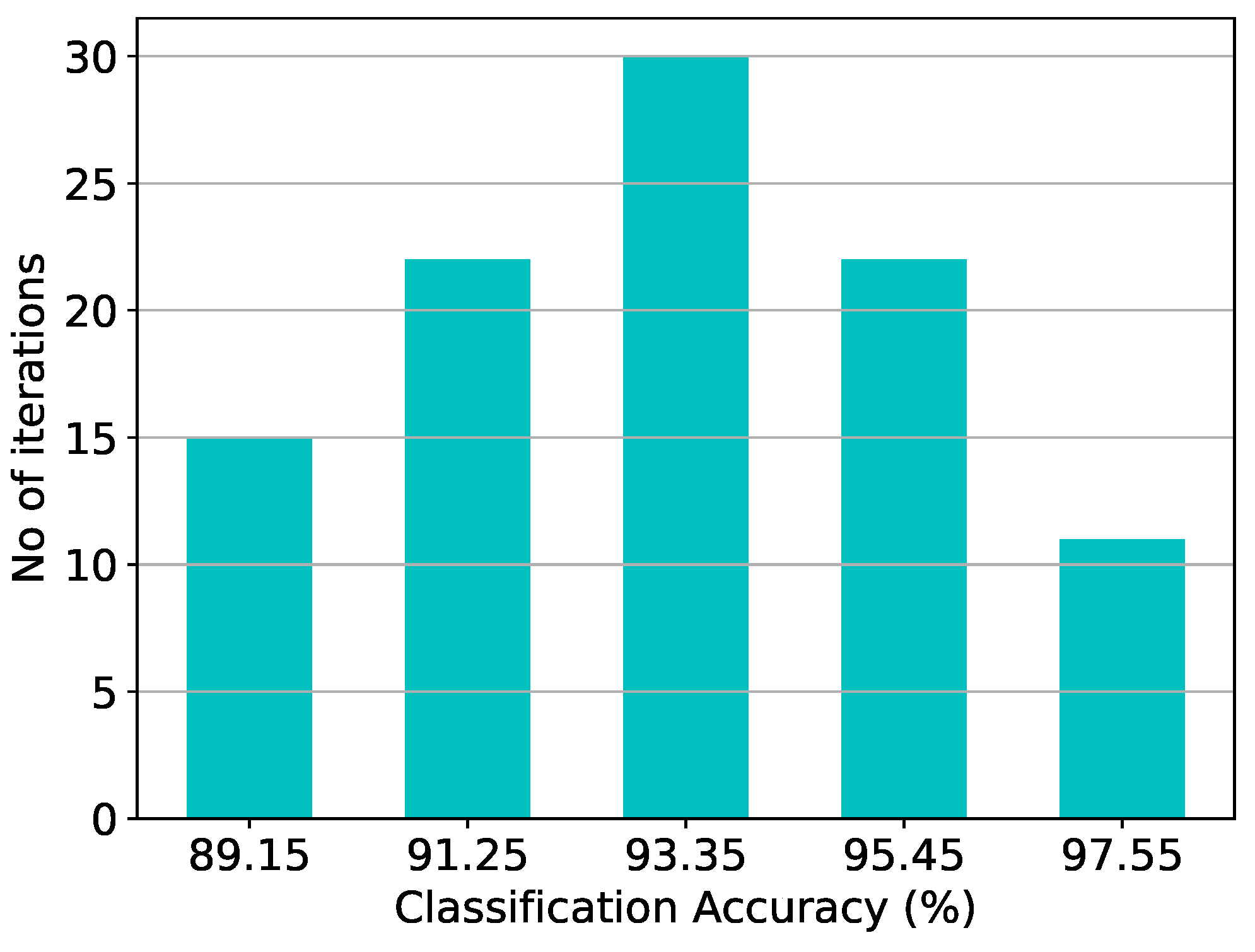
Figure 12.
Post-layout Monte Carlo simulation results of the GMM architecture on the thyroid disease detection dataset with and .
Figure 12.
Post-layout Monte Carlo simulation results of the GMM architecture on the thyroid disease detection dataset with and .
Figure 13.
An analog RBF-based classifier comprises 3 classes, 3 clusters per class, and 5 input dimensions.
Figure 13.
An analog RBF-based classifier comprises 3 classes, 3 clusters per class, and 5 input dimensions.
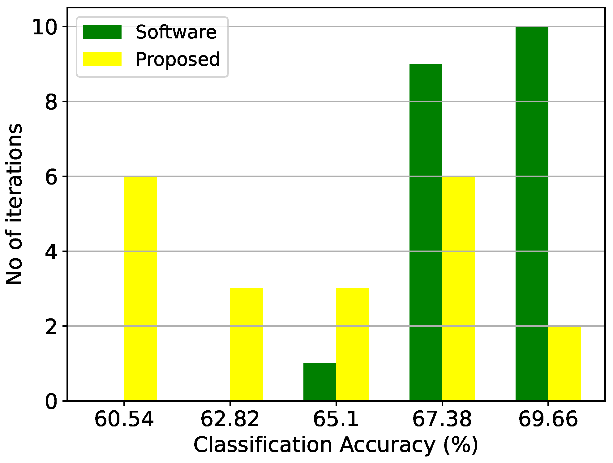
Figure 14.
Classification results of the RBF architecture and the equivalent software model on the thyroid disease detection dataset over 20 iterations.
Figure 14.
Classification results of the RBF architecture and the equivalent software model on the thyroid disease detection dataset over 20 iterations.
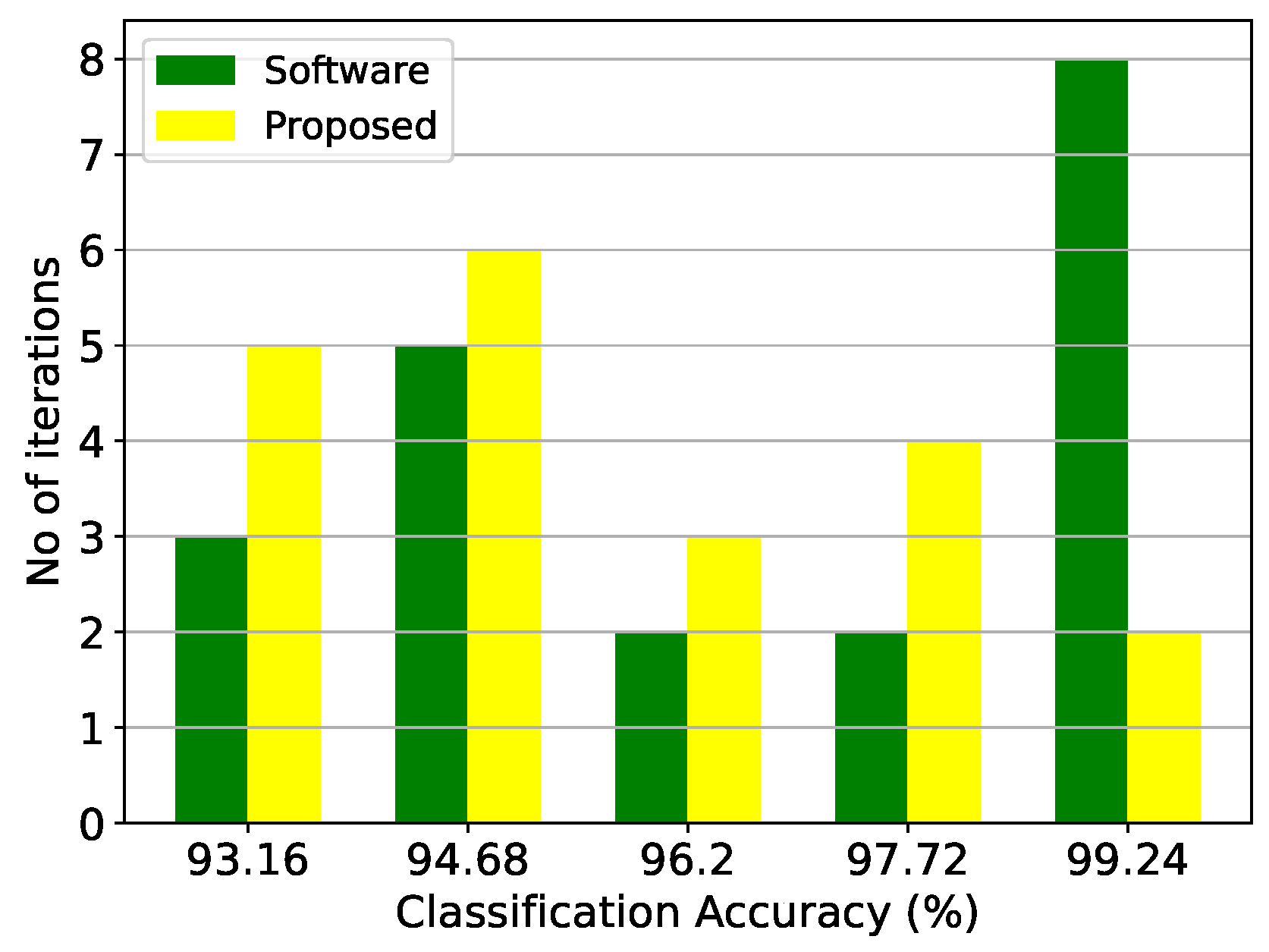
Figure 15.
Classification results of the RBF architecture and the equivalent software model on the epileptic seizure prediction dataset over 20 iterations.
Figure 15.
Classification results of the RBF architecture and the equivalent software model on the epileptic seizure prediction dataset over 20 iterations.
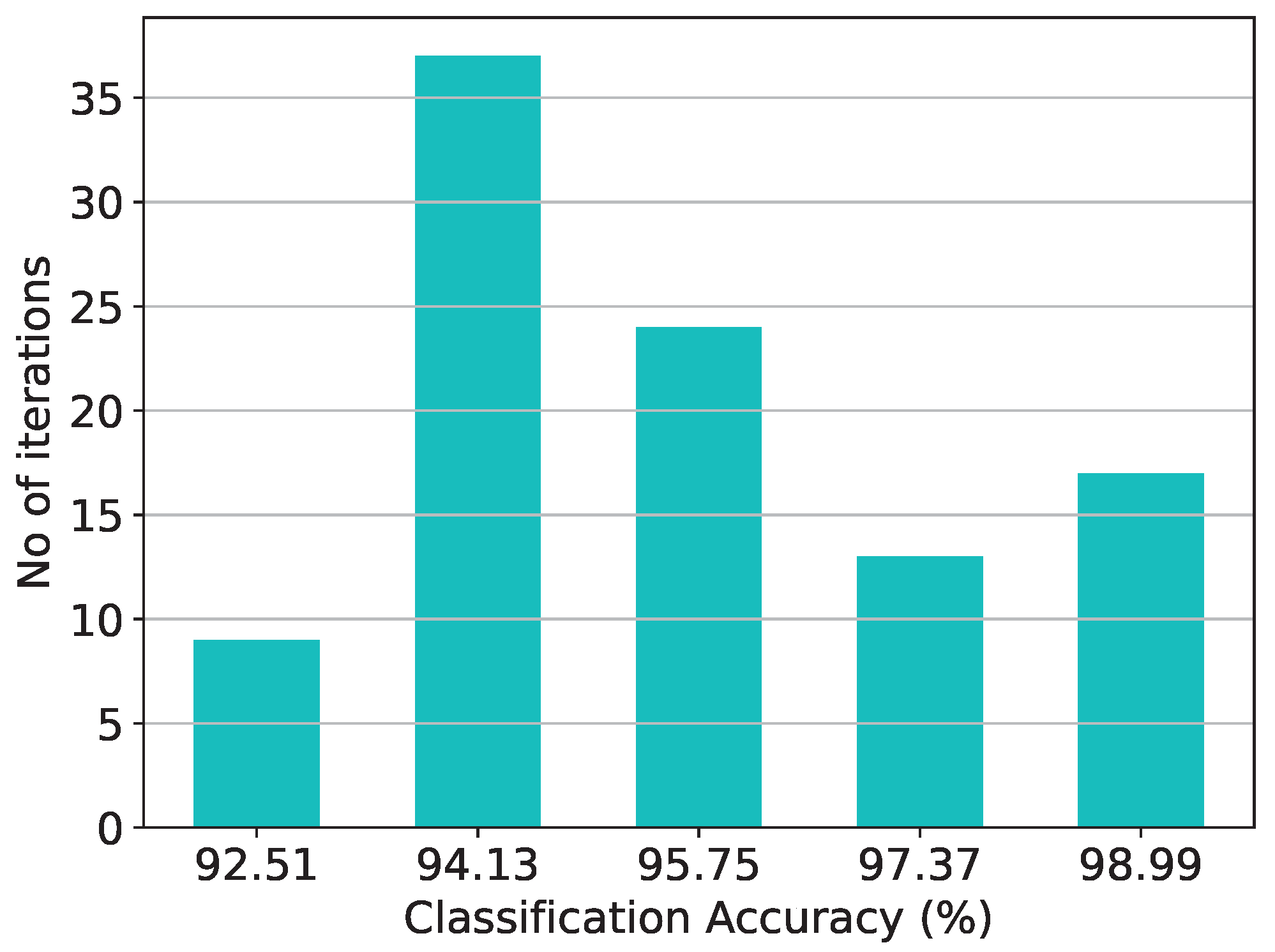
Figure 16.
Post-layout Monte Carlo simulation results of the RBF architecture on the thyroid disease detection dataset with and .
Figure 16.
Post-layout Monte Carlo simulation results of the RBF architecture on the thyroid disease detection dataset with and .
Figure 17.
An analog Bayesian classifier comprises 3 classes and 5 input dimensions.
Figure 17.
An analog Bayesian classifier comprises 3 classes and 5 input dimensions.
Figure 18.
Classification results of the Bayesian architecture and the equivalent software model on the thyroid disease detection dataset over 20 iterations.
Figure 18.
Classification results of the Bayesian architecture and the equivalent software model on the thyroid disease detection dataset over 20 iterations.
Figure 19.
Classification results of the Bayesian architecture and the equivalent software model on the epileptic seizure prediction dataset over 20 iterations.
Figure 19.
Classification results of the Bayesian architecture and the equivalent software model on the epileptic seizure prediction dataset over 20 iterations.
Figure 20.
Post-layout Monte Carlo simulation results of the Bayesian architecture on the thyroid disease detection dataset with and .
Figure 20.
Post-layout Monte Carlo simulation results of the Bayesian architecture on the thyroid disease detection dataset with and .
Figure 21.
An analog Threshold classifier comprises 2 classes and 5 input dimensions. The second class is the decision boundary for the threshold implementation.
Figure 21.
An analog Threshold classifier comprises 2 classes and 5 input dimensions. The second class is the decision boundary for the threshold implementation.
Figure 22.
Classification results of the threshold architecture and the equivalent software model on the thyroid disease detection dataset over 20 iterations.
Figure 22.
Classification results of the threshold architecture and the equivalent software model on the thyroid disease detection dataset over 20 iterations.
Figure 23.
Classification results of the threshold architecture and the equivalent software model on the epileptic seizure prediction dataset over 20 iterations.
Figure 23.
Classification results of the threshold architecture and the equivalent software model on the epileptic seizure prediction dataset over 20 iterations.
Figure 24.
Post-layout Monte Carlo simulation results of the threshold architecture on the thyroid disease detection dataset with and .
Figure 24.
Post-layout Monte Carlo simulation results of the threshold architecture on the thyroid disease detection dataset with and .
Figure 25.
An analog centroid classifier comprises 2 classes, 2 centroids in the first class, 1 centroid in the second class, and 5 input dimensions.
Figure 25.
An analog centroid classifier comprises 2 classes, 2 centroids in the first class, 1 centroid in the second class, and 5 input dimensions.
Figure 26.
Classification results of the centroid architecture and the equivalent software model on the thyroid disease detection dataset over 20 iterations.
Figure 26.
Classification results of the centroid architecture and the equivalent software model on the thyroid disease detection dataset over 20 iterations.
Figure 27.
Classification results of the centroid architecture and the equivalent software model on the epileptic seizure prediction dataset over 20 iterations.
Figure 27.
Classification results of the centroid architecture and the equivalent software model on the epileptic seizure prediction dataset over 20 iterations.
Figure 28.
Post-layout Monte Carlo simulation results of the centroid architecture on the thyroid disease detection dataset with and .
Figure 28.
Post-layout Monte Carlo simulation results of the centroid architecture on the thyroid disease detection dataset with and .
Figure 29.
The cascaded WTA circuit composed of two 3-neuron WTA circuits and one 2-neuron WTA circuit in cascaded connection. The outputs of the second WTA circuit are three currents in a digital one-hot representation; the two currents are summed up together and subsequently fed as input to the third WTA circuit along with the third output of the second WTA.
Figure 30.
An analog SVM classifier consists of M RBF cells and 2 classes. The RBF cells receive the input dimensions and generate the suitable RBF patterns utilizing the learned parameters. These derived RBF patterns correspond to the Support Vectors in the model. To convey the polarity of the Support Vectors to the classification block switches are employed. A WTA approach is implemented for contrasting the positive and negative magnitudes.
Figure 31.
Classification results of the SVM architecture and the equivalent software model on the thyroid disease detection dataset over 20 iterations.
Figure 31.
Classification results of the SVM architecture and the equivalent software model on the thyroid disease detection dataset over 20 iterations.
Figure 32.
Classification results of the SVM architecture and the equivalent software model on the epileptic seizure prediction dataset over 20 iterations.
Figure 32.
Classification results of the SVM architecture and the equivalent software model on the epileptic seizure prediction dataset over 20 iterations.
Figure 33.
Post-layout Monte Carlo simulation results of the SVM architecture on the thyroid disease detection dataset with and .
Figure 33.
Post-layout Monte Carlo simulation results of the SVM architecture on the thyroid disease detection dataset with and .
Table 1.
Bump circuit transistors’ dimensions.
Table 1.
Bump circuit transistors’ dimensions.
| NMOS Differential Block | W/L | Current Correlator | W/L |
|---|
| , | | , | |
| , | | , | |
| – | | , | |
| , | | - | - |
Table 2.
GMM-based CLF’s accuracy for thyroid disease detection dataset (over 20 iterations).
Table 2.
GMM-based CLF’s accuracy for thyroid disease detection dataset (over 20 iterations).
| Method | Best | Worst | Mean | Variance |
|---|
| Software | % | % | % | % |
| Hardware | % | % | % | % |
Table 3.
GMM-based CLF’s accuracy for epileptic seizure prediction dataset (over 20 iterations).
Table 3.
GMM-based CLF’s accuracy for epileptic seizure prediction dataset (over 20 iterations).
| Method | Best | Worst | Mean | Variance |
|---|
| Software | % | % | % | |
| Hardware | % | % | % | |
Table 4.
RBF CLF’s accuracy for thyroid disease detection dataset (over 20 iterations).
Table 4.
RBF CLF’s accuracy for thyroid disease detection dataset (over 20 iterations).
| Method | Best | Worst | Mean | Variance |
|---|
| Software | % | % | % | % |
| Hardware | % | % | % | % |
Table 5.
RBF CLF’s accuracy for epileptic seizure prediction dataset (over 20 iterations).
Table 5.
RBF CLF’s accuracy for epileptic seizure prediction dataset (over 20 iterations).
| Method | Best | Worst | Mean | Variance |
|---|
| Software | % | % | % | |
| Hardware | % | % | % | % |
Table 6.
Bayes CLF’s accuracy for thyroid disease detection dataset (over 20 iterations).
Table 6.
Bayes CLF’s accuracy for thyroid disease detection dataset (over 20 iterations).
| Method | Best | Worst | Mean | Variance |
|---|
| Software | % | % | % | % |
| Hardware | % | % | % | % |
Table 7.
Bayes CLF’s accuracy for epileptic seizure prediction dataset (over 20 iterations).
Table 7.
Bayes CLF’s accuracy for epileptic seizure prediction dataset (over 20 iterations).
| Method | Best | Worst | Mean | Variance |
|---|
| Software | % | % | % | % |
| Hardware | % | % | % | % |
Table 8.
Threshold CLF’s accuracy for thyroid disease detection dataset (over 20 iterations).
Table 8.
Threshold CLF’s accuracy for thyroid disease detection dataset (over 20 iterations).
| Method | Best | Worst | Mean | Variance |
|---|
| Software | % | % | % | % |
| Hardware | % | % | % | % |
Table 9.
Threshold CLF’s accuracy for epileptic seizure prediction dataset (over 20 iterations).
Table 9.
Threshold CLF’s accuracy for epileptic seizure prediction dataset (over 20 iterations).
| Method | Best | Worst | Mean | Variance |
|---|
| Software | % | % | % | % |
| Hardware | % | % | % | % |
Table 10.
Centroid-based CLF’s accuracy for thyroid disease detection dataset (over 20 iterations).
Table 10.
Centroid-based CLF’s accuracy for thyroid disease detection dataset (over 20 iterations).
| Method | Best | Worst | Mean | Variance |
|---|
| Software | % | % | % | % |
| Hardware | % | % | % | % |
Table 11.
Centroid-based CLF’s accuracy for epileptic seizure prediction dataset (over 20 iterations).
Table 11.
Centroid-based CLF’s accuracy for epileptic seizure prediction dataset (over 20 iterations).
| Method | Best | Worst | Mean | Variance |
|---|
| Software | % | % | % | % |
| Hardware | % | % | % | % |
Table 12.
SVM CLF’s accuracy for thyroid disease detection dataset (over 20 iterations).
Table 12.
SVM CLF’s accuracy for thyroid disease detection dataset (over 20 iterations).
| Method | Best | Worst | Mean | Variance |
|---|
| Software | % | % | % | % |
| Hardware | % | % | % | % |
Table 13.
SVM CLF’s accuracy for epileptic seizure prediction dataset (over 20 iterations).
Table 13.
SVM CLF’s accuracy for epileptic seizure prediction dataset (over 20 iterations).
| Method | Best | Worst | Mean | Variance |
|---|
| Software | % | % | % | % |
| Hardware | % | % | % | % |
Table 14.
Implemented analog classifiers’ performance comparison for thyroid disease detection dataset.
Table 14.
Implemented analog classifiers’ performance comparison for thyroid disease detection dataset.
| Classifier | Best | Worst | Mean | Power
Consumption | Processing
Speed | Energy per
Classification |
|---|
| GMM | | | | | | |
| RBF | | | | | | |
| Bayes | | | | 421 nW | | |
| Threshold | | | | | | |
| Centroid | | | | | | |
| SVM | | | | | | |
Table 15.
Implemented analog classifiers’ performance comparison for epileptic seizure prediction dataset.
Table 15.
Implemented analog classifiers’ performance comparison for epileptic seizure prediction dataset.
| Classifier | Best | Worst | Mean | Power
Consumption | Processing
Speed | Energy per
Classification |
|---|
| GMM | | | | 180 nW | | |
| RBF | | | | 231 nW | | |
| Bayes | | | | 123 nW | | |
| Threshold | | | | | | |
| Centroid | | | | 355 nW | | |
| SVM | | | | | | |
Table 16.
Analog classifiers’ comparison on the epileptic seizure prediction dataset.
Table 16.
Analog classifiers’ comparison on the epileptic seizure prediction dataset.
| Classifier | Best | Worst | Mean | Power
Consumption | Processing
Speed | Energy per
Classification |
|---|
| GMM | | | | 180 nW | | |
| RBF | | | | 231 nW | | |
| Bayes | | | | 123 nW | | |
| Threshold | | | | | | |
| Centroid | | | | 355 nW | | |
| SVM | | | | | | |
| RBF [27] | | | | | | |
| RBF-NN [29] | | | | 870 nW | | |
| SVM [30] | | | | | | |
| MLP [38] | | | | | | |
| K-means [43] | | | | | | |
| Fuzzy [45] | | | | 761 nW | | |
| SVR [51] | | | | W | | |
| LSTM [59] | | | | mW | | |


 and
and 


