VNF Migration in Digital Twin Network for NFV Environment

Abstract

Network Function Virtualization (NFV) allows for the dynamic provisioning of Virtual Network Functions (VNFs), adapting services to the complex and dynamic network environment to enhance network performance. However, VNF migration and energy consumption pose significant challenges due to the dynamic nature of the physical network. In order to maximize the acceptance rate of Service Function Chain Requests (SFCR), and reduce VNF migration and energy consumption as much as possible, we summarize several related factors such as the node hosting state, link hosting state, energy consumption, migrated nodes, and whether the mapping is successful. We define the Markov decision process by considering the factors mentioned above. Next, we design the VNF migration algorithm utilizing actor–critic models, graph convolution networks, and LSTM networks. In order to reduce the risk of trial and error during training and prediction in deep reinforcement learning scenarios, we designed a network architecture based on a digital twin (DT). In simulation experiments, compared with the FF algorithm that greedily selects the first available node, our AC_GCN algorithm significantly improves the acceptance rate of SFC requests by 2.9 times more than the FF algorithm in small topology experiments, and 27 times more than the FF algorithm in large topology experiments. Compared with the deep reinforcement learning (DRL) algorithm, which does not consider all the above factors together, for the small topology experiment, our AC_GCN algorithm outperforms the DRL algorithm in terms of request acceptance rate by 13%, underperforms compared to the DRL algorithm in terms of energy consumption by 3.8%, and underperforms compared to the DRL algorithm in terms of the number of migrated nodes for 22%; for the large topology experiment, our AC_GCN algorithm outperforms the DRL algorithm in terms of the request acceptance rate by 7.7%, outperforms the DRL algorithm in terms of energy consumption by 0.4%, and outperforms the DRL algorithm in terms of the number of migrated nodes by 1.6%.

1. Introduction

In traditional network architectures, network functions like firewalls, load balancers, intrusion detection systems, and content delivery servers are typically implemented in dedicated physical appliances. Each network function operates independently, leading to complex and inflexible network deployments that hinder the introduction of new services and the scaling of existing ones. To address these limitations, Service Function Chaining (SFC) introduces a dynamic and programmable approach to service delivery. Instead of relying on dedicated hardware appliances, SFC virtualizes network functions and orchestrates them in a logical chain. This chain represents the flow of network traffic through various services, with each function performing a specific task or processing step. SFC decouples network functions from the underlying hardware, and enables the deployment of these functions as virtual instances or software-based components. It provides a centralized management system for defining the order of functions, traffic steering policies, and necessary service-level agreements (SLAs). Service Function Chaining (SFC) enables the efficient chaining and orchestration of multiple network functions or services to meet specific requirements. It serves as a framework for deploying and managing a sequence of network functions as a unified service, enabling flexible and customizable service delivery. SFC revolutionizes the way network services are delivered and managed, offering flexibility and scalability to adapt swiftly to evolving business needs. In the context of 5G and future networks, the ability to dynamically adjust to network traffic, resource requirement, and load changes over time is crucial [1,2]. However, improper VNF deployment can lead to SFC failures and network downtime [1]. Simply re-instantiating a VNF on a physical node results in the loss of state information of the original VNF, causing the service flow information of the VNFs to accumulate in the SFCs and update continuously as the network operates. This simplistic instantiation approach disrupts network service continuity and incurs substantial reconfiguration costs [3,4]. To address these challenges effectively, a VNF migration framework that retains state information is the preferred solution [5].

There exists a significant correlation between VNF migration and the dynamic shifts in network traffic and resource demands. Virtualized network functions must possess the flexibility to scale both horizontally and vertically in response to varying workloads, ensuring efficient resource utilization. In the context of Network Function Virtualization (NFV), the network must dynamically allocate resources, responding to real-time demands presented by SFC requests. When network traffic surges, accompanied by increased resource requirements, there might be VNF migration. This migration occurs when the resource demands surpass the maximum capacity of the physical nodes or links. Conversely, during periods of reduced network traffic, some resources can be released to optimize cost-efficiency. However, such constraints can introduce unpredictable challenges to the network. For instance, as network traffic and resource demands persistently grow, frequent VNF migration can become a common occurrence. Recurring passive VNF migration introduces network instability, potentially impacting the user experience.

In order to increase the acceptance rate of SFC requests, reduce the frequency of VNF migrations, and decrease energy consumption, a proactive approach involves periodically migrating VNFs. By doing so, the NFV network can significantly increase the request acceptance rate and reduce migration and energy consumption as much as possible. One day is divided into discrete time slots, and VNFs are actively migrated at the beginning of each time slot based on the predicted network traffic for the upcoming period. A critical challenge in this approach revolves around the design of practical migration algorithms. These algorithms must strike a balance between increasing request acceptance rate and optimizing migration frequency and energy consumption.

Deep reinforcement learning (DRL) algorithms have found applications in NFV networks for modeling updates, seeking optimal solutions for resource allocation, and making decisions. Deep reinforcement learning algorithms have trial and error costs, and trial and error is untolerable in computer networks. Trial and error processes within computer networks can pose significant risks, potentially leading to irreparable damage. To mitigate these risks, a novel network architecture is required to separate the trial and error training phase from prediction. This approach ensures that network models are trained offline and thoroughly validated before deployment. Such a strategy reduces the potential for trial and error mishaps and enables deployment efficiency. Recently, digital twin (DT) networks have received substantial attention, as they enable network virtualization. They take virtual descriptions or digital representations of the real world to create mix-reality virtual worlds [6]. In our context, we introduce DT to capture the dynamic changes in VNF resource requirements in computer networks. We design a network architecture based on DT and DRL-based VNF migration algorithms to address the challenges posed by time-varying network traffic.

The main contributions of this paper can be summarized as follows:

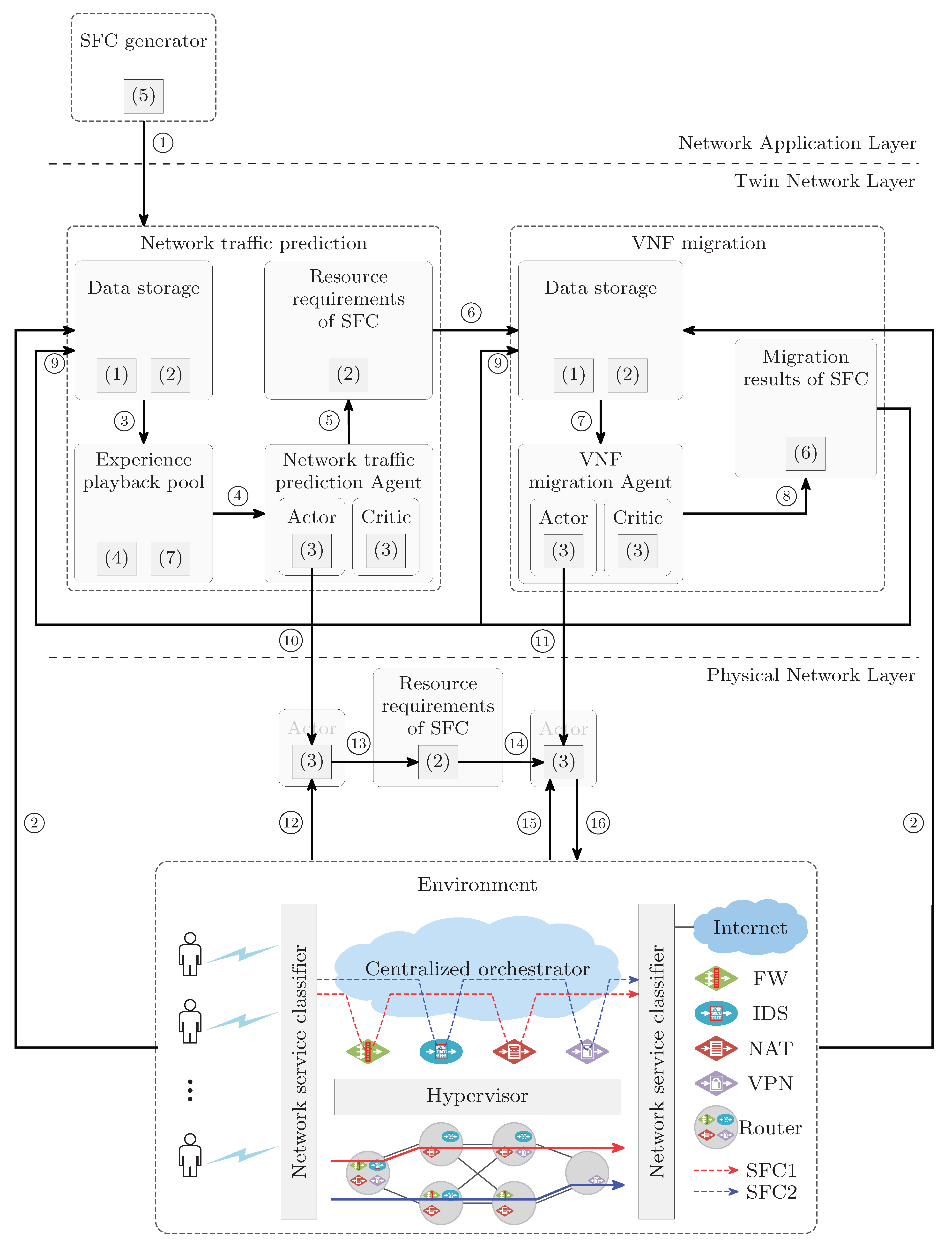
• Introducing the DT network architecture: In our approach, we integrate DT technology to construct a network architecture that faithfully simulates the real-time state and dynamic characteristics of the physical network. By mapping the physical network’s entities into the virtual realm, we design a DT network architecture tailored to handle time-varying network traffic efficiently.
• Addressing dynamic VNF migration: We tackle the challenge of VNF migration in the dynamic NFV network environment caused by fluctuating network traffic. To enhance the effectiveness of VNF migration decisions, we propose an algorithm called Agent based on Actor–Critic model and Graph Convolution Network (AC_GCN).
• DRL algorithm for efficient VNF migration: We introduce a DRL algorithm based on AC_GCN to determine the migration targets and formulate VNF migration strategies. The primary goal is to maximizing request acceptance rate and reduce migration frequency and energy consumption as much as possible.
• Performance analysis and key factors evaluation: In our study, we thoroughly analyze the performance of the proposed algorithms.

The remainder of this paper is structured as follows. Section 2 provides an overview of the most relevant research pertaining to traffic-aware VNF migration and digital twin network technology. In Section 3, we detail the problem model for traffic-aware VNF migration and introduce the architecture of the DT network. In Section 4, we outline our proposed algorithm for traffic-aware VNF migration, explaining its key components and methodology. In Section 5, we perform simulation experiments, and present the results of our simulation experiments. We analyze the outcomes across various algorithms and delve into the factors that influence the network availability. In Section 6, we present a discussion based on our research and experimentation. In Section 7, we summarize our findings and propose a plan for future work.

2. Related Work

Table 1. Overview of the related works.

Subject	Related Work	Scope	Problem	Objective	Algorithm or Method
VNF migration	Ref. [7]	NFV	NFV elasticity control	Reduce migration cost	heuristic
	Ref. [8]	NFV	VNF migration according to changing workload	Save energy	heuristic
	Ref. [9]	NFV	SFC placement in Mobile Edge Computing	Save energy	heuristic
	Ref. [10]	NFV	Time selection for Edge VNF placement	Reduce end-to-end latency	heuristic
	Ref. [11]	NFV	VNF placement in the edge network	Reduce end-to-end latency	heuristic
	Ref. [4]	NFV	VNF Migration in Data Center Networks	Resource optimization and delay reduction	heuristic
Traffic-aware VNF Migration	Ref. [12]	NFV	VNF migration in dynamic traffic	Dynamic network slicing	machine learning
	Ref. [13]	NFV	Request prediction in dynamic traffic	Resource reduction	CNN+LSTM+DRL
	Ref. [14]	NFV	VNF migration	Delay-optimized and resource-efficient	Ant Colony Optimization
	Ref. [15]	NFV	VNF migration in dynamic 5G networks	Time-average and cost-minimizing	Lyapunov optimization
	Ref. [16]	NFV	VNF migration in mobile edge network	Balance between the SFC latency and the migration cost	Markov approximation
	Ref. [17]	NFV	Resource allocation based on dynamic traffic load	Ensure performance isolation between VNFs	heuristic
Digital Twin Network	Ref. [18]	Network virtualization in 6G networks	Conceptual architecture for the 6G network	AI integration	Apply digital twin network
	Ref. [19]	Industrial Internet of Things	Instant wireless connectivity	Reliability and security	Apply digital twin network
	Ref. [20]	NFV	Root cause analysis	Availability and superiority	Digital twin network and hidden Markov model
	Ref. [21]	Industrial Internet of Things	Stochastic computation offloading and resource allocation	Long-term energy efficiency	Digital twin network and Lyapunov optimization
	Ref. [1]	NFV enabled Internet of Things	Network traffic prediction and VNF migration	Reduce the number of migrated VNFs and save energy	Digital twin network, DRL, and federated learning

presents an overview of the related works. The detailed descriptions on the related works are shown in the following paragraphs.

2.1. VNF Migration

The VNF migration problem generally refers to the process of migrating VNFs from one place to another due to specific reasons such as dynamic resource requirements and hardware maintenance [22]. During the migration, preserving the state consistency is important for accurate packet processing. Sun et al. [7] modeled the VNF migration problem as an ILP problem, and proposed a heuristic method to solve this problem with reduced migration cost and acceptable computation complexity. Eramo et al. [8] designed a VNF migration architecture considering its energy consumption, and proposed a heuristic algorithm-based method to determine the migration strategy. Badri et al. [9] jointly considered the QoS and energy consumption in edge networks, and proposed a modified algorithm to solve the formulated multistage stochastic program. The authors in [10,11] designed migration strategies in edge networks, aiming to minimize the end-to-end delay of SFC. The difference is that Cziva et al. [10] mainly focused on VNF migration timing and designed a dynamic rescheduling method based on the theory of optimal stopping. Song et al. [11] computed the optimal number of clusters in edge networks, and used a graph partitioning algorithm to minimize the number of VNFs to be migrated among clusters. Li et al. [4] aimed to minimize the end-to-end delay for all abnormal SFCs in data center networks.

2.2. Traffic-Aware VNF Migration

In the domain of Network Function Virtualization (NFV), software-defined networking (SDN), and digital twin networks (DTN), many research endeavors have explored the realm of traffic-aware Virtual Network Function (VNF) migration. These efforts aim to optimize VNF migration decisions by leveraging network traffic characteristics and meeting performance requirements.

Kumar et al. [12] introduced a data-driven, machine-learning-based slicing and allocation model that offers enhanced flexibility with Quality of Service (QoS) and that supports traffic-aware, reliable dynamic slicing. Azad et al. [13] presented a network slicing framework and incorporated a deep learning model, CNN-LSTM, to predict User Equipment (UE) requests within network slices, accounting for the dynamic nature of network traffic patterns. Bu et al. [14] proposed a mechanism for dynamically deploying customized network functions through NFV, contributing to the efficient adaptation of network services. In Xie et al. [15], the authors examined the effects of flow rate fluctuations in service requests, leading to potential service migrations and fluctuations in network queues (buffers). Their research addresses the cost-minimizing problem of VNF placement and routing within this dynamic environment while considering service migration and queue backlog stability. Qin et al. [16] took into account variations in network topology to optimize the system performance cost-effectively. Their focus lies in the problem of Service Function Chain (SFC) migration in dynamic networks, aiming to strike a balance between SFC latency and migration costs. Chintapalli et al. [17] introduced a dynamic, joint resource allocation scheme that considers each VNF’s input traffic rate as an input parameter. It dynamically adjusts cache ways and allocates bandwidth resources among VNFs to avoid performance interference.

2.3. Digital Twin Network

In the realm of DT networks, various research endeavors have explored innovative applications and architectures. These references shed light on the diverse capabilities and advantages of DT-based systems.

Wu et al. [23] presented a comprehensive survey of DTN to explore the potentiality of DT. Shen et al. [18] proposed an innovative DT-based network virtualization architecture. This architecture enhances network management capabilities and facilitates efficient service delivery to end-users. Lu et al. [19] introduced a novel DT wireless network model that incorporates DTs into wireless networks. This integration address issues related to unreliable long-distance communication between users and base stations. It synchronizes user data with base stations and constructs corresponding DTs. Wang et al. [20] presented an architecture tailored for NFV environments based on DT. It leverages historical knowledge to accurately identify anomaly-fault dependencies, thus saving significant time and computational costs. Dai et al. [21] focused on designing the topology of Industrial Internet of Things (IIoT) networks using DT. It monitors network characteristics, such as dynamic resource changes and random task arrivals. Liu et al. [1] designed a DT-based network architecture, with a particular emphasis on solving network traffic prediction challenges within the NFV environment. These referenced works represent significant contributions in the realms of traffic-aware VNF migration and DT networks. They have paved the way for our research, inspiring the design of an NFV architecture rooted in DT principles to address VNF migration challenges. Our work introduces the model and algorithm based on DT and AC_GCN for VNF migration. This approach can capture the dynamic nature of VNF resources.

3. Network Architecture Design and Problem Statement

3.1. The Architecture of the DT Network in NFV Environment

Figure 1 and Figure 2 illustrate our proposed virtualization architecture, which leverage DT networks to enhance network management and service provisioning. In this architecture, the NFV network infrastructure corresponds to the physical network layer within the DTN architecture. Key functions of the NFV network, such as service function chain mapping, virtual network function migration, and network traffic prediction, are executed by the multiple service mapping models within the twin network layer. The generation of the service function chain is managed by the network application layer.

To optimize data communication between the twin network layer and the physical network layer, we employ a replication of the actor model within the physical network layer. This approach serves a dual purpose: reducing communication volume and enhancing data security. Specifically, we place two actor networks at the physical network layer. One actor is replicated from the actor network of the agent responsible for network traffic prediction, while the other actor is replicated from the actor network of the agent responsible for VNF migration. At the physical network layer, these actors are deployed to predict network traffic and facilitate VNF migration, respectively.

In Figure 1’s twin network layer, the agent responsible for network traffic prediction was explored in our previous work. In this paper, we focus on discussing and exploring the agent responsible for VNF migration, providing a detailed overview of its functionality.

In Figure 1, we can identify the following steps: ➀ Input SFCs; ➁ Copy; ➂ Calculate reward and save information; ➃ Extract historical network traffic data; ➄ Predict network traffic; ➅ Input requirement of SFCs and update data for the environment; ➆ Input environmental data or calculate reward; ➇ Calculate the migration of SFC requests; ➈ Input the deployment results of SFC migration; ➉⑪ Copy model and parameters; ⑫ Input environmental data and historical network traffic data; ⑬ Predict network traffic; ⑭ Input the requirements of SFC; ⑮ Input the environmental data; ⑯ Calculate the migration of SFC requests and input the results into the environment.

3.2. Problem Model

3.2.1. System Model

(1)

Physical Network

DT models the network as a discrete time slotted system. A graph $G^{PN}=\left(N^P,L^P\right)$ is used to represent the physical network, where $N^P$ denotes physical nodes in the physical network, and $L^P$ denotes physical links in the physical network.

We use a 3-tuple to characterize physical network in the DT network.

$$D{T}_P\left(q\right)=\left.\left\{D{T}_{PN}\left(q\right),D{T}_{PL}\left(q\right),M_{topo}\right.\right\}$$

(1)

where $D{T}_{PN}\left(q\right)$ is the set of physical nodes on the physical network, $D{T}_{PL}\left(q\right)$ is the set of physical links on the physical network, and $M_{topo}$ is the topology of the physical network.

We use a 3-tuple to characterize physical nodes in the DT network.

$$D{T}_{PN}\left(q,i\right)=\left\{n_{cpu}\left(i\right),n_{storage}\left(i\right),M_{support}\left(i\right)\right\}$$

(2)

where $n_{cpu}\left(i\right)$ represents the available CPU resources of the physical node i, $n_{storage}\left(i\right)$ represents the available storage resources of the physical node i, and $M_{support}\left(i\right)$ represents the set of supported VNFs for the physical node i.

We use a 2-tuple to characterize physical links in the DT network.

$$D{T}_{PL}\left(q,j\right)=\left\{l_{bw}\left(j\right),l_{lat}\left(j\right)\right\}$$

(3)

where $l_{bw}\left(j\right)$ represents the available bandwidth resource of the physical link j, and $l_{lat}\left(j\right)$ represents the latency of the physical link j.

(2)

SFC request

A graph $G^{VN}=\left(N^V,L^V\right)$ is used to represent each SFC request, where $N^V$ denotes VNFs of each SFC request, and $L^V$ denotes virtual links of each SFC request. We use a 3-tuple to characterize SFC request i in the DT network.

$$D{T}_V\left(q,i\right)=\left\{D{T}_{VN}\left(i\right),D{T}_{VL}\left(i\right),Lat\left(i\right)\right\}$$

(4)

where $D{T}_{VN}\left(i\right)$ is the set of all VNFs on the SFC request i, $D{T}_{VL}\left(i\right)$ is the set of all virtual links on the SFC request i, and $Lat\left(i\right)$ represents the end to end delay limit of SFC request i.

We use a 3-tuple to characterize the VNF of the SFC request in the DT network.

$$D{T}_{VN}\left(t,i,j\right)=\left\{r_{cpu}\left(i,j\right),r_{storage}\left(i,j\right),e_{cpu}\left(i,j\right)\right\}$$

(5)

where $r_{cpu}\left(i,j\right)$ represents the required CPU resource for VNF j on the SFC request i in time slot t, $r_{storage}\left(i,j\right)$ represents the required storage resource for VNF j of SFC request i in time slot t, and $e_{cpu}\left(i,j\right)$ represents the embedded node for VNF j of SFC request i.

We use a 2-tuple to characterize the virtual link of SFC requests in the DT network.

$$D{T}_{VL}\left(t,i,j\right)=\left\{r_{bw}\left(i,j\right),e_{path}\left(i,j\right)\right\}$$

(6)

where $r_{bw}\left(i,j\right)$ represents the required bandwidth resource of virtual link j of SFC request i in time slot t, and $e_{path}\left(i,j\right)$ represents the embedded path for virtual link j of SFC request i.

3.2.2. Problem Formulation

In this paper, we aim to maximize request acceptance rate, reducing both the number of migrated nodes and energy consumption as much as possible. The objective is as follows:

$$Minimize\sum _{q=1}^N\sum _{i=1}^M\left({\eta }_1·e\left(q,i\right)+{\eta }_2·n_{mig}\left(q,i\right)-{\eta }_3·x\left(q,i\right)\right),$$

(7)

where ${\eta }_1$, ${\eta }_2$ and ${\eta }_3$ are constant coefficients, N represents the number of time slots divided in one day, M represents the number of SFC requests, $e\left(q,i\right)$ represents the energy consumption of SFC request i in time slot q, $n_{mig}\left(q,i\right)$ represents the migrated nodes of SFC request i in time slot q, and $x\left(q,i\right)$ represents whether SFC request i is mapped successfully or not, where the value is 1 in case of success and the value is 0 otherwise.

The constraints align with those from previous literature, such as [1,24,25]. The constraints include the following: each VNF can only be mapped to one physical node; each virtual link can only be mapped to one physical path; when the virtual link is remapped, the VNFs on it must be mapped to the corresponding physical node of the physical link where the virtual link is located; the resource (e.g., CPU, storage, or bandwidth) constraints can not be exceeded; the end-to-end delay limit of the SFC cannot be exceeded; and so on.

4. AC and GCN-Based Agent

The agent, known as AC_GCN, operates on the principles of actor–critic control. This approach involves two Neural Networks (NN) optimized using gradient descent and the value function algorithm, respectively.

4.1. Framework of Markov Decision Process (MDP)

In a standard reinforcement learning (RL) process, an MDP model serves as a foundational framework. Our MDP model comprises three primary components, including state, action, and reward.

4.1.1. State

The state is a comprehensive representation that encompasses both the resources of the physical network and the requirements and the embeddings of SFCs. Mathematically, the state can be expressed as

$$S\left(q\right)={\left(\begin{array}{c}{r}_{cpu\_remain}\left(1\right),\dots ,r_{cpu\_remain}\left(C\right),\hfill \\ r_{storage\_remain}\left(1\right),\dots ,r_{storage\_remain}\left(C\right),\hfill \\ r_{bw\_remain}\left(1\right),\dots ,r_{bw\_remain}\left(L\right),r_{lat}\left(1\right),\dots ,r_{lat}\left(L\right),\hfill \\ e_{cpu}\left(1,1\right),\dots ,e_{cpu}\left(M,D_M\right),\hfill \\ e_{path}\left(1,1\right),\dots ,e_{path}\left(M,L_M\right),\hfill \\ M_{support}\left(1\right),\dots ,M_{support}\left(C\right),M_{topo}\hfill \end{array}\right)}^T.$$

(8)

In Equation (8), C represents the number of physical nodes, L represents the number of physical links, M represents the number of SFC requests, $D_i$ represents the number of VNFs in SFC request i, and $L_i$ represents the number of virtual links in SFC request i. $n_{cpu\_remain}\left(i\right)$, $n_{storage\_remain}\left(i\right)$, $l_{lat}\left(j\right)$, and $l_{bw\_remain}\left(j\right)$ represent the available resources of the CPU of physical node i, the available storage of physical node i, the latency of the physical link j, and the available bandwidth of the physical link j, respectively. $e_{cpu}\left(i,j\right)$ represents the embedded node for VNF j in SFC request i. $e_{path}\left(i,j\right)$ represents the embedded physical path for virtual link j in SFC request i. $M_{support}\left(i\right)$ represents the set of supported VNFs for physical node i, and $M_{topo}$ represents the adjacency matrix for the topology of the physical network.

4.1.2. Action

The action corresponds to the migration scheme for each VNF within each SFC. The action includes the VNFs to be migrated and the physical nodes and physical paths to be migrated to. Formally, the action is represented as

$$a\left(q\right)=A\left(S\left(q\right)\right)=\left(s_{mig},s_{vnf\_embed},s_{vl\_embed}\right),$$

(9)

where $A\left(S\left(q\right)\right)$ represents the migration scheme under state $S\left(q\right)$, $s_{mig}$ represents the set of the VNFs to be migrated, $s_{vnf\_embed}$ represents the set of the embed objective for VNFs, and $s_{vl\_embed}$ represents the set of the embed objective for virtual links.

4.1.3. Reward

The reward reflects the impact of the action within the physical network under a specific state. Our primary objectives include maximizing the successful migration rate while reducing migration frequency and energy consumption.

In order to provide a more detailed assessment of mapping results, we introduce two distinct components, penalty and award. The penalty value represents the associated cost of the migration, and the award value is mainly related to whether the migration is successful or not.

The difference between award and penalty (incentive minus cost) is utilized as an evaluation metric for the migration scheme, offering a comprehensive assessment of its advantages and disadvantages.

(1)

Penalty

The cost $c\left(q\right)$ encompasses penalties associated with energy consumption, VNF migration frequency, and SFC request rejection.

(a)

The first scenario

In scenarios where the mapping of SFC request i succeeded in the previous time slot but failed in the next time slot, the penalty encompasses various factors, including the failure of SFC request mapping for the next time slot, the number of failed nodes and links associated with each SFC request, and the punitive measure applied to originally successful mappings in the previous time slot. The penalty can be expressed as

$$c\left(q,i\right)=s_{penalty}+p_{all\_node}\left(q,i\right)+p_{all\_link}\left(q,i\right)+c\left(q-1,i\right),$$

(10)

where $s_{penalty}$ represents a constant coefficient and $p_{all\_node}\left(q,i\right)$ represents the penalty for the failed node within the SFC request i in time slot q, and it is calculated as

$$p_{all\_node}\left(q,i\right)=\sum _{j=0}^{D_i-1}{p}_{node}\left(q,i,j\right),$$

(11)

where $D_i$ represents the number of VNFs in SFC request i, $p_{node}\left(q,i,j\right)$ represents the penalty for failed VNF j of SFC request i in time slot q. It can be calculated as

$$p_{node}\left(q,i,j\right)=\left\{\begin{array}{c}0,\mathrm{if}\mathrm{physical}\mathrm{node}e\left(j\right)\mathrm{can}\mathrm{carry}\mathrm{vnf}j\hfill \\ s_{node\_unit\_penalty}·\frac{r_{cpu}\left(i,j\right)-n_{cpu\_remain}\left(e\left(j\right)\right)}{n_{cpu}\left(e\left(j\right)\right)},\mathrm{otherwise}\hfill \end{array}\right.,$$

(12)

where $s_{node\_unit\_penalty}$ represents a constant coefficient for the failed mapping of the node, $r_{cpu}\left(i,j\right)$ represents the requested CPU of VNF j in SFC request i, $e\left(j\right)$ represents the physical node to which VNF j is mapped, $n_{cpu}\left(e\left(j\right)\right)$ represents the maximum capacity of the CPU in physical node $e\left(j\right)$, and $n_{cpu\_remain}\left(e\left(j\right)\right)$ represents the residual capacity of the CPU in physical node $e\left(j\right)$.

In Equation (10), $p_{all\_link}\left(q,i\right)$ represents the penalty for failed links within SFC request i, and it is calculated as

$$p_{all\_link}\left(q,i\right)=\sum _{j=0}^{L_i-1}{p}_{link}\left(q,i,j\right),$$

(13)

where $p_{link}\left(q,i,j\right)$ is calculated as

$$p_{link}\left(q,i,j\right)=\left\{\begin{array}{c}0,\mathrm{if}\mathrm{virtual}\mathrm{link}j\mathrm{mapping}\mathrm{success}\hfill \\ s_{link\_unit\_penalty},\mathrm{otherwise}\hfill \end{array}\right.,$$

(14)

where $s_{link\_unit\_penalty}$ is a constant coefficient.

(b)

The second scenario In scenarios where the mapping of SFC request i failed in the previous and next time slot, the penalty associates with the failure of SFC request mapping in the next time slot, as well as the failed nodes and links. It is calculated as

$$c\left(q,i\right)=s_{penalty}+p_{all\_node}\left(q,i\right)+p_{all\_link}\left(q,i\right).$$

(15)

(c)

The third scenario In scenarios where the mapping of SFC request i failed in the previous time slot but succeeded in the next time slot, the penalty is associated with energy consumption and the failed mapping of the SFC request i in the previous time slot. It is calculated as

$$c\left(q,i\right)=e_{penalty}·e\left(q,i\right)-c\left(q-1,i\right),$$

(16)

where $e_{penalty}$ is a constant coefficient for energy consumption and $e\left(q,i\right)$ represents the energy consumption of SFC request i in the next time slot q, and it can be calculated as

$$e\left(q,i\right)=\sum _{j=0}^{D_i-1}\left[p_{min}+\left(p_{max}-p_{min}\right)·\frac{r_{cpu}\left(i,j\right)}{n_{cpu}\left(e\left(j\right)\right)}\right],$$

(17)

where $p_{max}$ and $p_{min}$ represent the maximum and minimum amount of energy consumed by physical node $e\left(j\right)$, respectively.

(d)

The fourth scenario In scenarios where the mapping of SFC request i succeeded in the previous and next time slot, the penalty should take into account both energy consumption and the number of migrated nodes. It is calculated as

$$c\left(q,i\right)=e_{penalty}·e\left(q,i\right)+n_{penalty}·n_{mig}\left(q,i\right),$$

(18)

where $n_{penalty}$ represents a constant coefficient for node migration and $n_{mig}\left(q,i\right)$ represents the total number of migrated physical nodes in SFC request i, and it is calculated as

$$n_{mig}\left(q,i\right)=\sum _{j\in N^V\left(i\right)}\sum _{m\in N^P}\sum _{n\in N^{P}andm\ne n}Z\left(i,j,m,n\right),$$

(19)

where $Z\left(i,j,m,n\right)$ represents whether to migrate VNF j in SFC request i from physical node m to physical node n in time slot q. $N^P$ represents the set of physical nodes in the physical network, and $N^V\left(i\right)$ represents the set of virtual nodes in the SFC request i.

(2)

Award The award value for the action taken in the next time slot is determined by comparing the award in the previous time slot with the award in the next time slot.

(a)

The first scenario In scenarios where the mapping of SFC request i succeeded in the previous time slot but failed in the next time slot, the award is determined as the negative value of the successful mapping award, and it can be expressed as

$$w\left(q,i\right)=-s_{award},$$

(20)

where $s_{award}$ represents a constant coefficient for successful mapping.

(c)

The second scenario In scenarios where the mapping of SFC request i failed in the previous and the next time slot, Equation (21) serves to define the award:

$$w\left(q,i\right)=-s_{award}+r\left(q-1,i\right).$$

(21)

(c)

The third scenario In scenarios where the mapping of SFC request i failed in the previous time slot but succeeded in the next time slot, Equation (22) serves to define the award:

$$w\left(q,i\right)=s_{award}+r\left(q-1,i\right).$$

(22)

(d)

The fourth scenario In scenarios where the mapping of SFC request i succeeded in the previous and the next time slot, Equation (23) serves to define the award:

$$w\left(q,i\right)=s_{award}.$$

(23)

(3)

Reward In the mapping scheme of SFC request i, the reward is calculated as the difference between the award and the penalty, and it can be represented as

$$r\left(q,i\right)=w\left(q,i\right)-c\left(q,i\right).$$

(24)

4.2. Structure of the Agent for VNF Migration

4.2.1. Interactions among Components

The data storage is extracted from environment and updated by the predicted network traffic. The AC_GCN agent interacts with both the data storage and the deployment of SFC, as depicted in Figure 3. Throughout the training process, the AC_GCN agent dynamically adapts to the evolving environment, continuously updating its decision-making capabilities.

4.2.2. Structure of the AC_GCN Agent

The AC_GCN agent employs the Policy Gradient algorithm for action determination. Policy Gradient algorithms fall into two categories: strategy networks with a stochastic policy gradient and strategy networks with a deterministic policy gradient. We utilize the stochastic policy gradient. As illustrated in Figure 3, the AC_GCN agent’s architecture comprises two neural networks: the actor network and the critic network. During the training process, the actor network is updated using the policy gradient method, and the critic network employs the value function to iteratively update its parameters.

4.2.3. Structure of Actor Network

The actor network in our model follows a sequence-to-sequence (seq2seq) architecture [26], as illustrated in Figure 3. This architecture combines Graph Convolutional Networks (GCN) and Long Short-term Memory (LSTM) cells. In Figure 3, the encoder consists of both a GCN model and an LSTM model, while the decoder comprises an LSTM layer followed by a fully connected layer. The output of the seq2seq model undergoes normalization using the Softmax function.

The model takes three primary inputs: the SFCs, the topology of the physical network, and features related to the physical network. The actor network takes these inputs to generate action probabilities for each physical node concerning each VNF.

4.2.4. Structure of Critic Network

The critic network serves as a value estimator network. It employs LSTM layers connected to a fully connected layer (dense layer). This network predicts the Lagrangian value for actions based on the current policy.

4.3. Update Methods for Parameters of the Neural Networks

In an RL approach, an agent interacts with an environment with the objective of discovering optimal actions within a Markov Decision Process (MDP). As the agent takes actions in the environment, it receives rewards. This iterative process forms the basis of the agent’s training to determine the most advantageous decisions [27].

During the RL training process, we employ the actor–critic model. This model aims to identify the optimal policy by concurrently executing value and policy iteration. The actor, representing the executed policy, generates actions, while the critic approximates the value function to evaluate these actions [28].

The actor and critic functions are implemented as distinct neural networks with separate sets of parameters. The actor network is denoted as $\pi$. It utilizes parameters denoted as $\theta$. Meanwhile, the critic network, responsible for approximating the value function, employs parameters denoted as ${\theta }_v$ [27]. In the actor network, the updating of parameters $\theta$ is carried out using the Policy Gradient algorithm, which minimizes the loss $loss\_actor$ associated with it. Meanwhile, in the critic network, the parameters ${\theta }_v$ are updated using the value function algorithm, optimizing its associated loss $loss\_critic$.

The Lagrangian function, denoted as $J_L^{\pi }\left(\theta \right)$ (i.e., $loss\_actor$), serves as the objective function. To compute the weights $\theta$ and optimize the objective function, we employ a combination of Monte-Carlo Policy Gradients and stochastic gradient descent. The updates to weights $\theta$ proceed as follows:

$${\theta }_{k+1}={\theta }_k+\alpha ·{\nabla }_{\theta }{J}_L^{\pi }\left(\theta \right).$$

(25)

The gradient is estimated through Monte-Carlo sampling, involving the drawing of B samples. To mitigate gradient variance, we incorporate a baseline estimator [29], denoted as $b\left(s\right)$, in the formula. ${\nabla }_{\theta }{J}_L^{\pi }\left(\theta \right)$ can be expressed as

$${\nabla }_{\theta }{J}_L^{\pi }\left(\theta \right)\approx \frac{1}{B}\sum _{j=1}^B\left(L\left(p_j,s_i\right)+\gamma ·b_{{\theta }_v}\left(p_r,s_i\right)·S\left(p_j,s_i\right)-L\left(p_{i-1},s_{i-1}\right)\right)·{\nabla }_{\theta }log{\pi }_{\theta }\left(p_j,s_i\right).$$

(26)

The Lagrangian value, denoted as $L\left(p_j,s_i\right)$, corresponds to the loss associated with the mapping result $p_j$ in state $s_i$. It is equivalent to the negative value of reward, and the reward is defined in Equation (24). $log{\pi }_{\theta }\left(p_j,s_i\right)$ denotes a log operation for the probability value of each node computed for the actor network. $L\left(p_{i-1},s_{i-1}\right)$ represents the Lagrangian value of mapping result $p_{i-1}$ in state $s_{i-1}$. The placement $p_r$ represents the optimal sample chosen from the actor network in state $s_i$. It is assessed by the critic network to derive an evaluation denoted as $b_{{\theta }_v}\left(p_r,s_i\right)$, which is then utilized as the baseline. We set $S\left(p_j,s_i\right)$ to 1 when the remapping result $p_j$ in state $s_i$ is successful; otherwise, it takes the value 0.

The parameters ${\theta }_v$ of the critic network are trained through a loss function (i.e., $loss\_critic$), which is based on the mean squared error objective. This loss function is defined as

$$\ell \left({\theta }_v\right)=\frac{1}{B}\sum _{j=1}^B{∥b_{{\theta }_v}\left(p_j,s_i\right)-L\left(p_j,s_i\right)∥}^2.$$

(27)

4.4. Key Processes of the AC_GCN Agent

4.4.1. Predicting Process of the AC_GCN Agent

In our proposed network architecture (as shown in Figure 1), we train the actors in the twin network layer for both network traffic prediction and VNF migration. After training, these actors are replicated in the physical network layer.

During the training of the actor for VNF migration, the required input data are obtained from the data storage. When using the trained actor for predictions, the necessary input data are retrieved from the network environment in the physical network layer. The prediction process described below can be utilized for both training and prediction processes.

The prediction process is illustrated in Figure 4.

In step 1-1, apply the predicted network traffic for the upcoming time slot $next\_traffic$ to the physical network, resulting in the generation of a new physical network state $env1$.

In step 1-2, within the physical network $env1$, calculate the adjacency matrix $support$ and feature matrix $feature$. The feature matrix $feature$ contains essential information about all physical nodes, including the VNFs they can support and the remaining CPU capacity.

In step 1-3, take the adjacency matrix $support$, the feature matrix $feature$, and the SFC requests $SFCR$ and input them into the GCN located within the encoder of the actor network. The GCN leverages its prediction function to generate an output tensor $out$.

In step 1-4, perform a dot-multiplication operation between the tensor $out$ generated in step 1-3 and the VNF support matrix $VNF\_SUPPORT\_MATRIX$ of the physical nodes. This operation results in the probability matrix $output$, which is used to assess the availability of VNFs at each physical node;

In step 1-5, utilize the tensor $output$ obtained in step 1-4 to determine the selection probability for each VNF in each SFC. This calculation yields the probability matrix $input\_embedding$.

In step 1-6, input both the SFC requests $SFCR$ and the probability matrix $input\_embedding$ from step 1-5 into the LSTM layer of the encoder within the actor network. This process allows us to make the prediction $encoder\_output$ and obtain the state $encoder\_final\_state$.

In step 1-7, take the prediction $encoder\_output$ and the state $encoder\_final\_state$ obtained in step 1-6 and input them into the LSTM layer of the decoder within the actor network. This process involves the LSTM’s predicting operation, resulting in the prediction $decoder\_output$ and the state $decoder\_state$.

In step 1-8, feed the prediction $decoder\_output$ from step 1-7 into the fully connected (FC) layer of the decoder within the actor network. The output of this step is the tensor $decoder\_logit$;

In step 1-9, apply the Softmax operation to the tensor $decoder\_logit$ obtained in step 1-8. The output of this operation yields the output $decoder\_softmax$;

In step 1-10, select the N samples with the highest probability based on the output tensor $decoder\_softmax$ from step 1-9. The result of this selection is the tensor $decoder\_exploration$.

4.4.2. Training Process of the AC_GCN Agent

We train the actors within the twin network layer, and the training process encompasses the integration of the prediction process. Specifically, during the actor training for VNF migration, it is imperative to incorporate the prediction process discussed in Section 4.4.1. The training data are sourced from the data storage, as depicted in Figure 1.

The training process involves a specific loop, and a single iteration of this loop is illustrated in Figure 5. As we progress through the loop, we follow the steps outlined next. This loop represents the core of our training procedure, where we iterate through the steps described to refine our model.

In step 2-1, perform a categorical distribution operation on the output tensor $decoder\_softmax$ from step 1-9. This operation results in the matrix $prob$.

In step 2-2, within the network state corresponding to the previous time slot, apply the predicted network traffic from the previous time slot $previous\_traffic$. This step produces the physical network state $env2$, as well as the penalty $previous\_penalty$ and award $previous\_award$ for the previous time slot.

In step 2-3, combine the output $decoder\_exploration$ from step 1-10, the penalty $previous\_penalty$, the award $previous\_award$, the SFC requests $SFCR$, and the network state $env2$ to calculate the best sample. This calculation results in the placement $best\_placement$, the Lagrangian value $best\_Lagrangian$, and the embedding state $best\_embed\_state$ for the best sample.

In step 2-4, perform Softmax calculation on the optimal sample obtained in step 2-3 according to the categorical distribution matrix $prob$ from step 2-1, and obtain the tensor $softmax$. Then, perform a log operation and an averaging operation to the tensor $softmax$, resulting in the tensor $best\_log\_softmax\_mean$.

In step 2-5, subtract the penalty for the previous time slot $previous\_penalty$ by the award for the previous time slot $previous\_award$, as computed in step 2-2. This subtraction yields the Lagrangian value $previous\_Lagrangian$ for the previous time slot.

In step 2-6, input the placement $best\_placement$ of the best sample from step 2-3 into the critic network. This step allows us to obtain the evaluation $baseline$.

In step 2-7, utilize the Lagrangian value $best\_lagrangian$ obtained from step 2-3, the Boolean value $best\_embed\_state$ obtained from step 2-3 that identifies the success or failure of the remapping process, and the output tensor $baseline$ from step 2-6 to calculate a new tensor using Equation (28). The result of this calculation can be expressed as

$$td\_target=best\_Lagrangian-\gamma ·baseline·best\_embed\_state.$$

(28)

In step 2-8, subtract the tensor $td\_target$ obtained in step 2-7 by the Lagrangian value $previous\_Lagrangian$ from step 2-5. This subtraction results in the difference $advantage$.

In step 2-9, multiply the difference $advantage$ from step 2-8 by the output tensor $log\_softmax\_mean$ from step 2-4. Subsequently, take the average of this multiplication to calculate the loss tensor $loss\_actor$.

In step 2-10, input the loss $loss\_actor$ obtained in step 2-9 into the optimizer of the actor network. This step involves updating the parameters of the actor network based on the calculated loss $loss\_actor$.

In step 2-11, calculate the loss tensor $loss\_critic$ by taking the squared difference between the output $best\_Lagrangian$ from step 2-3 and the evaluation $baseline$ from step 2-6.

In step 2-12, input the loss tensor $loss\_critic$ obtained in step 2-11 into the optimizer of the critic network. This step leads to the updating of the parameters of the critic network.

4.4.3. Predicting Process of GCN

The predicting process of the GCN is shown in Figure 6.

In step 3-1, input the adjacency matrix $support$ and the feature matrix $feature$ obtained from step 1-2 into Graph Convolution Layer 1, and obtain the resulting tensor $output1$.

In step 3-2, input the tensor $output1$ obtained from step 3-1 and the feature matrix $feature$ obtained from step 1-2 into Graph Convolution Layer 2, and obtain the resulting tensor $output2$.

4.4.4. Training Process of GCN

The training process of the GCN is shown in Figure 7.

In step 4-1, input the probability matrix $input\_embedding$ obtained from step 1-5 and the tensor $decoder\_softmax$ from step 1-9 into the function $loss\_func$, and output the resulting tensor $loss\_GCN$.

In step 4-2, input the tensor $loss\_GCN$ obtained from step 4-1 into the GCN optimizer, and update the parameters of the GCN.

4.4.5. Function $loss\_func$

The function $loss\_func$ is shown in Figure 8.

In step 5-1, combine the parameters of Graph Convolution Layer 1 (GCL1) and Graph Convolution Layer 2 (GCL2) to generate the tensor $var\_list$.

In step 5-2, apply regularization to the tensor $var\_list$ from step 5-1 to obtain the refined tensor $regularized\_var\_list$.

In step 5-3, calculate a weighted sum of the tensor $regularized\_var\_list$ from step 5-2 to obtain tensor $loss\_weight$.

In step 5-4, perform cross-entropy and averaging operations on the probability matrix $input\_embedding$ from step 1-5 and the tensor $decoder\_softmax$ from step 1-9, resulting in tensor $loss\_ave\_node$.

In step 5-5, add tensor $loss\_ave\_node$ from step 5-4 to tensor $loss\_weight$ from step 5-3 to produce tensor $loss$, and return the resulting tensor $loss$.

5. Performance Evaluation

We evaluate the performance of the AC_GCN agent in a TensorFlow-based environment. All simulations were conducted on a computer with an i9-13900HX CPU and 16 GB DDR5 RAM.

5.1. Simulation Setting

To evaluate our proposed approach for optimizing the VNF migration problem, we conducted a comprehensive experimental study in two distinct environments of varying sizes. The small infrastructure has 100 nodes and 1485 edges, and the large infrastructure has 200 nodes and 995 edges. The topologies of these physical networks were randomly generated. Key parameters for nodes and links included the following:

• Node CPU capacity range: [7, 10];
• Link bandwidth range: [400, 1000];
• Link latency range: [1, 4].

In our experiment, we used eight different types of Virtual Network Functions (VNFs), and their specifications are detailed in

Table 2. VNF Properties.

VNF ID	CPU Cores Required	BW Required	Processing Latency
1	1	10	1
2	2	10	1
3	2	10	1
4	2	20	2
5	2	20	2
6	2	20	2
7	1	20	2
8	1	20	2

. The VNFs were randomly selected to create the SFC requests.

For the small infrastructure, we generated 25 SFC requests, while for the large infrastructure, we generated 50 SFC requests. The migration interval, which represents the length of a time slot, was set to 2 h.

Additional crucial parameters can be found in

Table 3. Values of constant coefficient for equations.

Equation ID	Constant Coefficient	Value
(10)	$s_{penalty}$	1500
(12)	$s_{node\_unit\_penalty}$	60
(14)	$s_{link\_unit\_penalty}$	60
(16)	$e_{penalty}$	5
(17)	$p_{max}$	300
(17)	$p_{min}$	200
(18)	$n_{penalty}$	10
(20)	$s_{award}$	15,000
(26)	B	300
(28)	$\gamma$	0.9

and

Table 4. Other main parameters.

Hyper Parameter	Value
Learning Rate of Actor Network	0.1
Learning Rate of Critic Network	0.0001
Number of Time Slots	12
Number of Layers in LSTM	2
Number of Hidden Dimensions in LSTM	100
Discard Rate	0.2
Training Times	201

.

5.2. Compared Algorithms

In our experiments, we constructed neural networks using GCN layers, LSTM layers, and FC layers. Our novel approach, named AC_GCN, was compared against two other algorithms:

• DRL algorithm: This method employs a DRL model to generate SFC deployment [30].
• FF algorithm: In this approach, VNF migration involves selecting the First-Fit Network Function instance on a physical node for each VNF [31].

5.3. Experiment and Simulation Results

In the prediction phase, we replicated the optimal neural network generated during the training process and applied it to the physical network layer for migration tasks.

The loss values during the training process are depicted in Figure 9. The results of the prediction process for both the small and large infrastructures are illustrated in Figure 10 and Figure 11, respectively.

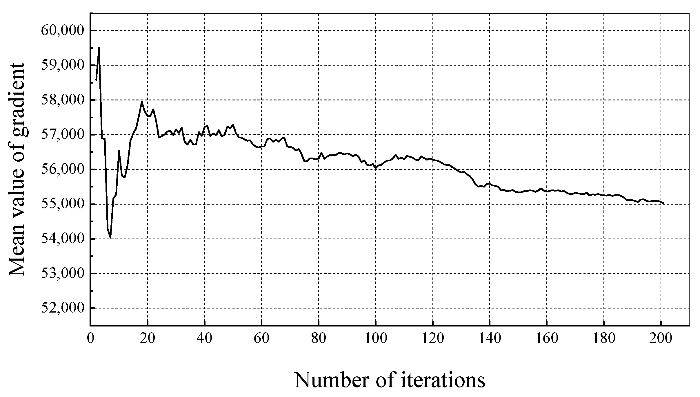
5.3.1. Convergence of AC_GCN during Training

First, to investigate the learning process of the bare Sequence-to-Sequence model, we conducted preliminary experiments. In Figure 9, we present the learning history of the agent on the large infrastructure. For each iteration, we introduce the mean values of loss for the actor network in the AC_GCN agent.

From the observations in Figure 9, it is evident that the learning algorithm of the seq2seq agent has nearly converged after 201 iterations.

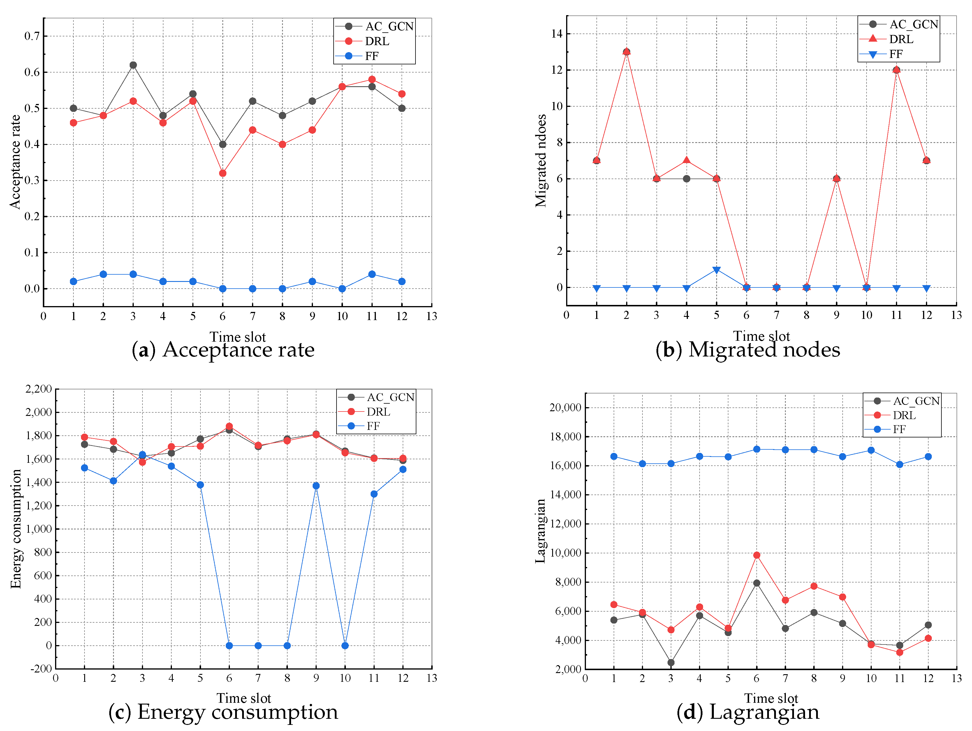
5.3.2. Comparison of Lagrangian and Other Metrics during Performance

In Figure 10a and Figure 11a, our algorithm exhibits higher acceptance rates in each time slot when compared to the other two algorithms in most instances. In Figure 10b,c and Figure 11b,c, our algorithm’s performance in every time slot is comparable to the DRL algorithm, while being significantly higher than that of the FF algorithm. The FF algorithm exhibits a low request acceptance rate, and few SFC requests are successfully migrated. Consequently, it records a low count of migrated nodes and exhibits reduced energy consumption. Figure 10d and Figure 11d provide valuable insights into the Lagrangian values associated with each algorithm’s performance in various time slots. Notably, our algorithm generally exhibits lower Lagrangian values when compared to both the DRL and FF algorithms.

This superior performance can be attributed to three key factors. First, during the training process, we employ a higher penalty for request rejection, and the success of the SFC migration is rewarded and penalized from different perspectives in penalties and awards. This encourages the algorithm to prioritize acceptance, which directly contributes to the improved acceptance rates observed. Second, our algorithm leverages GCN technology to better assimilate and adapt to the real-time state of the physical network. This learning mechanism results in a higher request acceptance rate compared to the other algorithms. Third, the agent is trained with the goal of minimizing the Lagrangian value, which takes the negative value of the reward. In the AC_GCN algorithm, the reward definition includes two parts: punishment and award. The definition of punishment mainly includes punishment for failed nodes, failed links, energy consumption and node migration; the definition of award mainly includes awards for successful migration of SFCs. The comparison of our proposed algorithm AC_GCN with the DRL and FF algorithms is shown in

Table 5. Comparison of the algorithms.

Algorithm	Request Acceptance	Availability of Node	Availability of Link	Requirement Satisfied	Energy Consumption	Migration
DRL	no	yes	yes	yes	yes	no
AC_GCN	yes	yes	yes	yes	yes	yes
FF	no	no	no	yes	no	no

. The trained AC_GCN agent can achieve better Lagrangian values, which makes AC_GCN perform better in terms of request acceptance, energy consumption, and the number of migrated nodes. However, when the request acceptance rate increases significantly, it comes at the expense of other metrics, such as energy consumption and the number of nodes migrated. From a holistic perspective, our AC_GCN algorithm emerges as the top performer.

6. Discussion

This paper addresses the complex challenge of VNF migration in dynamic network traffic scenarios. Our primary objective is to minimize migration penalties, which encompass penalties related to migrated nodes, energy consumption, and the occurrence of failed SFC migration. To address this problem effectively, we propose a new solution, AC_GCN.

In the training phase, we select the AC_GCN agent with the lowest Lagrangian value, ensuring optimal performance. In the prediction phase, we harness the trained agent to forecast deployment scenarios for VNF migrations.

We provide a comprehensive analysis of AC_GCN, create a TensorFlow-based environment, and conduct simulations to assess the solution’s performance. The results of our evaluation demonstrate that our solution excels in achieving our objectives.

Notably, we observe the convergence of AC_GCN during the training process, affirming its feasibility and efficacy. Overall, our solution significantly enhances rewards.

7. Conclusions

In this work, we study the VNF migration problem in a DT network. First, we establish a network architecture of the NFV network to adapt to the real-time VNF resource dynamic situation based on DT. Second, we convert multiple objectives for VNF migration into multiple factors, such as the node hosting state, link hosting state, energy consumption, migrated nodes, and request acceptance. We introduce an exciting extension to enhance the policy by fully defining an MDP. In that case, as migration decisions are made step-by-step, the agent is able to learn from multidimensional states, instead of inferencing it from a single input. Third, an AC_GCN algorithm is proposed to perform the migration of VNFs. The simulation results show that our proposed method for VNF migration has a higher acceptance rate and plays a positive role in guaranteeing more efficient energy savings and reduced migration.

In this paper, we use historical data to train actors at the twin network layer, then replicate the trained actors from the digital twin network layer to the physical network layer to implement network traffic prediction and VNF migration. When the services provided by SFC need to change significantly, the actor at the physical network layer will not be able to work effectively. Therefore, it is necessary to further optimize the training and prediction mechanisms so that the DT network can adapt to large changes in the services provided by the SFC (e.g., in terms of service type, combination of sub-functions in SFC request, resource requirements, latency requirements, etc.).

For the issue of VNF migration in dynamic network traffic, we have provided a complete overall architecture by integrating the DT network. We effectively integrate multiple factors, including request acceptance rate, energy consumption, and the number of migration nodes, offering a solution for defining rewards in the MDP model. The proposed AC_GCN algorithm provides a detailed solution to the VNF migration problem.

References

1. Liu, Q.; Tang, L.; Wu, T.; Chen, Q. Deep Reinforcement Learning for Resource Demand Prediction and Virtual Function Network Migration in Digital Twin Network. IEEE Internet Things J. 2023. early access. [Google Scholar] [CrossRef]
2. Ren, B.; Gu, S.; Guo, D.; Tang, G.; Lin, X. Joint Optimization of VNF Placement and Flow Scheduling in Mobile Core Network. IEEE Trans. Cloud Comput. 2022, 10, 1900–1912. [Google Scholar] [CrossRef]
3. Liu, Y.; Lu, Y.; Li, X.; Yao, Z.; Zhao, D. On Dynamic Service Function Chain Reconfiguration in IoT Networks. IEEE Internet Things J. 2020, 7, 10969–10984. [Google Scholar] [CrossRef]
4. Li, B.; Cheng, B.; Liu, X.; Wang, M.; Yue, Y.; Chen, J. Joint Resource Optimization and Delay-Aware Virtual Network Function Migration in Data Center Networks. IEEE Trans. Netw. Serv. Manag. 2021, 18, 2960–2974. [Google Scholar] [CrossRef]
5. Qu, K.; Zhuang, W.; Ye, Q.; Shen, X.; Li, X.; Rao, J. Dynamic Flow Migration for Embedded Services in SDN/NFV-Enabled 5G Core Networks. IEEE Trans. Commun. 2020, 68, 2394–2408. [Google Scholar] [CrossRef]
6. Wang, F.Y.; Qin, R.; Li, J.; Yuan, Y.; Wang, X. Parallel Societies: A Computing Perspective of Social Digital Twins and Virtual–Real Interactions. IEEE Trans. Comput. Soc. Syst. 2020, 7, 2–7. [Google Scholar] [CrossRef]
7. Sun, C.; Bi, J.; Meng, Z.; Yang, T.; Zhang, X.; Hu, H. Enabling NFV Elasticity Control With Optimized Flow Migration. IEEE J. Sel. Areas Commun. 2018, 36, 2288–2303. [Google Scholar] [CrossRef]
8. Eramo, V.; Miucci, E.; Ammar, M.; Lavacca, F.G. An Approach for Service Function Chain Routing and Virtual Function Network Instance Migration in Network Function Virtualization Architectures. IEEE/ACM Trans. Netw. 2017, 25, 2008–2025. [Google Scholar] [CrossRef]
9. Badri, H.; Bahreini, T.; Grosu, D.; Yang, K. Energy-Aware Application Placement in Mobile Edge Computing: A Stochastic Optimization Approach. IEEE Trans. Parallel Distrib. Syst. 2020, 31, 909–922. [Google Scholar] [CrossRef]
10. Cziva, R.; Anagnostopoulos, C.; Pezaros, D.P. Dynamic, Latency-Optimal vNF Placement at the Network Edge. In Proceedings of the IEEE INFOCOM 2018—IEEE Conference on Computer Communications, Honolulu, HI, USA, 16–19 April 2018; pp. 693–701. [Google Scholar] [CrossRef]
11. Song, S.; Lee, C.; Cho, H.; Lim, G.; Chung, J.M. Clustered Virtualized Network Functions Resource Allocation based on Context-Aware Grouping in 5G Edge Networks. IEEE Trans. Mob. Comput. 2020, 19, 1072–1083. [Google Scholar] [CrossRef]
12. Kumar, N.; Ahmad, A. Machine Learning-Based QoS and Traffic-Aware Prediction-Assisted Dynamic Network Slicing. Int. J. Commun. Netw. Distrib. Syst. 2022, 28, 27–42. [Google Scholar] [CrossRef]
13. Jalalian, A.; Yousefi, S.; Kunz, T. Network slicing in virtualized 5G Core with VNF sharing. J. Netw. Comput. Appl. 2023, 215, 103631. [Google Scholar] [CrossRef]
14. Bu, C.; Wang, J.; Wang, X. Towards delay-optimized and resource-efficient network function dynamic deployment for VNF service chaining. Appl. Soft Comput. 2022, 120, 108711. [Google Scholar] [CrossRef]
15. Xie, Y.; Wang, S.; Wang, B.; Xu, S.; Wang, X.; Ren, J. Online algorithm for migration aware Virtualized Network Function placing and routing in dynamic 5G networks. Comput. Netw. 2021, 194, 108115. [Google Scholar] [CrossRef]
16. Qin, Y.; Guo, D.; Luo, L.; Zhang, J.; Xu, M. Service function chain migration with the long-term budget in dynamic networks. Comput. Netw. 2023, 223, 109563. [Google Scholar] [CrossRef]
17. Chintapalli, V.R.; Adeppady, M.; Tamma, B.R.; Franklin, A. RESTRAIN: A dynamic and cost-efficient resource management scheme for addressing performance interference in NFV-based systems. J. Netw. Comput. Appl. 2022, 201, 103312. [Google Scholar] [CrossRef]
18. Shen, X.; Gao, J.; Wu, W.; Li, M.; Zhou, C.; Zhuang, W. Holistic Network Virtualization and Pervasive Network Intelligence for 6G. IEEE Commun. Surv. Tutor. 2022, 24, 1–30. [Google Scholar] [CrossRef]
19. Lu, Y.; Huang, X.; Zhang, K.; Maharjan, S.; Zhang, Y. Low-Latency Federated Learning and Blockchain for Edge Association in Digital Twin Empowered 6G Networks. IEEE Trans. Ind. Inform. 2021, 17, 5098–5107. [Google Scholar] [CrossRef]
20. Wang, W.; Tang, L.; Wang, C.; Chen, Q. Real-Time Analysis of Multiple Root Causes for Anomalies Assisted by Digital Twin in NFV Environment. IEEE Trans. Netw. Serv. Manag. 2022, 19, 905–921. [Google Scholar] [CrossRef]
21. Dai, Y.; Zhang, K.; Maharjan, S.; Zhang, Y. Deep Reinforcement Learning for Stochastic Computation Offloading in Digital Twin Networks. IEEE Trans. Ind. Inform. 2021, 17, 4968–4977. [Google Scholar] [CrossRef]
22. Yi, B.; Wang, X.; Li, K.; Das, S.k.; Huang, M. A comprehensive survey of Network Function Virtualization. Comput. Netw. 2018, 133, 212–262. [Google Scholar] [CrossRef]
23. Wu, Y.; Zhang, K.; Zhang, Y. Digital Twin Networks: A Survey. IEEE Internet Things J. 2021, 8, 13789–13804. [Google Scholar] [CrossRef]
24. Wang, H.; Wu, Y.; Min, G.; Xu, J.; Tang, P. Data-driven dynamic resource scheduling for network slicing: A Deep reinforcement learning approach. Inf. Sci. 2019, 498, 106–116. [Google Scholar] [CrossRef]
25. Wang, Q.; Alcaraz-Calero, J.; Ricart-Sanchez, R.; Weiss, M.B.; Gavras, A.; Nikaein, N.; Vasilakos, X.; Giacomo, B.; Pietro, G.; Roddy, M.; et al. Enable Advanced QoS-Aware Network Slicing in 5G Networks for Slice-Based Media Use Cases. IEEE Trans. Broadcast. 2019, 65, 444–453. [Google Scholar] [CrossRef]
26. Sutskever, I.; Vinyals, O.; Le, Q.V. Sequence to Sequence Learning with Neural Networks; MIT Press: Cambridge, MA, USA, 2014; pp. 3104–3112. [Google Scholar]
27. Geursen, I.L.; Santos, B.F.; Yorke-Smith, N. Fleet planning under demand and fuel price uncertainty using actor-critic reinforcement learning. J. Air Transp. Manag. 2023, 109, 102397. [Google Scholar] [CrossRef]
28. Grondman, I.; Busoniu, L.; Lopes, G.A.D.; Babuska, R. A Survey of Actor-Critic Reinforcement Learning: Standard and Natural Policy Gradients. IEEE Trans. Syst. Man Cybern. Part C (Appl. Rev.) 2012, 42, 1291–1307. [Google Scholar] [CrossRef]
29. Sutton, R.S.; Barto, A.G. Introduction to Reinforcement Learning; MIT Press: Cambridge, MA, USA, 1998. [Google Scholar]
30. Solozabal, R.; Ceberio, J.; Sanchoyerto, A.; Zabala, L.; Blanco, B.; Liberal, F. Virtual Network Function Placement Optimization With Deep Reinforcement Learning. IEEE J. Sel. Areas Commun. 2020, 38, 292–303. [Google Scholar] [CrossRef]
31. Kumaraswamy, S.; Nair, M.K. Bin packing algorithms for virtual machine placement in cloud computing: A review. Int. J. Electr. Comput. Eng. (IJECE) 2019, 9, 512. [Google Scholar] [CrossRef]
Figure 1. General network architecture.
Electronics 12 04324 g001
Figure 2. Parts expansion diagram for Figure 1.
Electronics 12 04324 g002
Figure 3. Structure of the agent for VNF migration.
Electronics 12 04324 g003
Figure 4. The prediction process of AC_GCN agent.
Electronics 12 04324 g004
Figure 5. The training process of AC_GCN agent.
Electronics 12 04324 g005
Figure 6. Predicting process of GCN.
Electronics 12 04324 g006
Figure 7. Training process of GCN.
Electronics 12 04324 g007
Figure 8. Function of loss calculation.
Electronics 12 04324 g008
Figure 9. Mean values of gradient for actor network in the training process.
Electronics 12 04324 g009
Figure 10. Results of the small infrastructure during performance.
Electronics 12 04324 g010
Figure 11. Results of the large infrastructure during performance.
Electronics 12 04324 g011