Photonic Multiple Microwave Frequency Measurement System with Single-Branch Detection Based on Polarization Interference

Abstract

A photonic microwave frequency measurement system with single-branch detection based on polarization interference is proposed. In this scheme, a 15-line non-flat optical frequency comb (OFC) based on sawtooth signal modulation via a Mach–Zehnder modulator is generated. The intercepted microwave signal with multiple-frequency components can be measured by frequency down-conversion with this simple structure. This system can measure the multi-tone microwave signals in real time. The single-branch detection makes the system a simple and compact structure and avoids the unbalanced variation, as in a two-branches scheme. The blind area of the system can be solved by adjusting the comb-line spacing of the OFC. A simulation is carried out and related discussion is given. The result reveals that it can measure multi-tone microwave signals with a resolution of less than 2 MHz over 0.1–12 GHz.

1. Introduction

Instantaneous microwave frequency (IFM) measurement is a topic of interest in some fields such as communications, electronic warfare, cognitive radio systems, etc. Traditional electrical frequency measurement systems are restricted by limitations such as limited frequency measurement range and problems of electromagnetic interference (EMI) [1]. Featuring with broad bandwidth, high flexibility, immunity to EMI and high speed, photonics-based frequency measurement has attracted great attention in recent years [2,3].

Generally, the photonics-assisted IFM system can be divided into three categories based on frequency-to-power mapping [4,5,6], frequency-to-time mapping [7,8], and frequency-to-space mapping [9,10,11,12,13]. The majority of frequency-to-power mapping systems rely on producing an amplitude comparison function (ACF), which constructs the relationship between the unknown microwave frequency and the optical or electrical power. The ACF can also be built by polarization [4], interferometers [5] or dispersive mediums [6]. A polarization-multiplexing Mach–Zehnder modulator (PM-MZM) and a polarization controller (PC) are jointly used to realize polarization interference based on optical power monitoring with an error of ±0.2 GHz over 4.4–8.7 GHz and 4.4–8.5 GHz [4]. In Ref. [5], a $S{i}_3{N}_4$ ring-assisted Mach–Zehnder interferometer is used as a frequency discriminator to achieve a high resolution of less than ±0.037 GHz error over 5–39 GHz. These systems are usually adjustable and have simple structure features, but it has the drawback of only measuring single-tone signals. Another solution is the photonics-based frequency-to-time mapping measurement. This scheme uses the unique characteristics of some optical devices to display microwave frequencies in time domain such as multiple central wavelengths [7] or silicon photonic scanning devices [8]. The above approach was further extended to measure multi-tune signals. For example, a photonic compressive receiver with an effective measurement range of 42 GHz and a multiple-frequency resolution of 1.2 GHz is proposed [7]. An integrated silicon photonic scanning filter is used to establish the relationship between the unknown microwave frequency and time domain with a high resolution of 375 MHz and a low measurement error of 237.3 MHz over 1–30 GHz [8]. However, it cannot tackle with the real-time pulse signals and features with its relatively low resolution (i.e., hundreds of megahertz). The frequency-to-space mapping method is widely adopted in photonic channelizers due to its real-time characteristics and the capability of measuring multi-tone broadband signals. In this case, the input microwave signals with high frequency are down-converted by a channelizer via Fabry–Pérot filters [9], fiber Bragg grating [10] or optical frequency combs (OFC) [11,12,13]. Among them, the OFC-based method is popular because of its lower resolution. In Ref. [12], a system based on a digital-signal-driven OFC can measure the unknown signals over 0–50 GHz in simulation. An experimental setup based on the spacing and profile of OFC is also proposed with less than 2 MHz over 1–40 GHz [13]. However, they are complex systems, such as ones using multiple photodetectors (PD) and modulators, which is difficult to achieve on a chip.

In this paper, we propose an IFM method based on polarization interference and sawtooth signal modulation. The system features a compact structure of single-branch detection and simple operation, which makes the system easy to implement. Moreover, the system is capable of measuring multi-tone signals, and because of the non-flat OFC, the input signals are down-converted into many channels with a narrow bandwidth. Therefore, only low-speed post-processing devices are needed to achieve the proposed system. The simulation results demonstrate an impressive measurement with high resolution less than 2 MHz over 0.1–12 GHz.

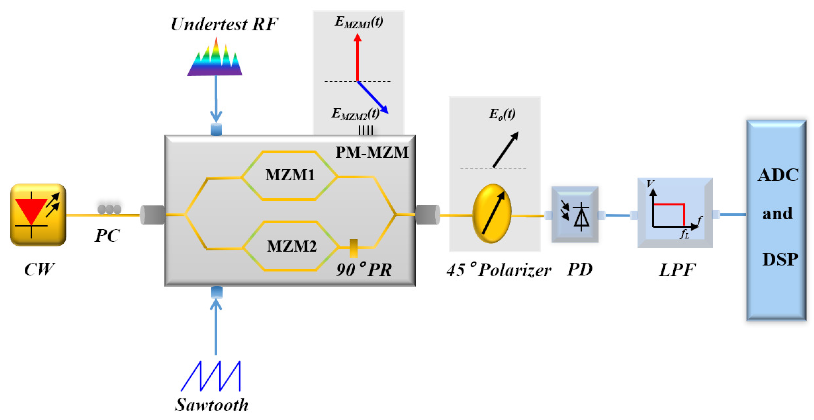
2. Theory and Principle

Figure 1 shows the schematic diagram of the proposed IFM system. The system mainly consists of one continuous wave laser (CW), one integrated PM-MZM (including two sub-MZMs, namely MZM1 and MZM2), one polarization rotator (PR), one 45-degree polarizer, one PD and one low-pass filter (LPF). The light emitted from a continuous wave laser can be expressed as $E_{in}\left(t\right)=E_{0}exp\left(j2\pi f_{c}t\right)$, where $E_0$ and $f_c$ denote the amplitude and frequency of the light signal, respectively. It is firstly input into a PM-MZM, in which the light wave is divided into two paths. In the upper path, the unknown multi-tone radio frequency (RF) signal $V_{RF}\left(t\right)=V_{n}cos\left(2\pi f_{n}t\right)(n=1,2,3,\cdots )$ is received and fed to the MZM1, biased at null peak point to achieve carrier-suppressed double-sideband modulation (CS-DSB). By applying the small modulation condition, only the $\pm 1st$ order sideband is considered and the modulated signal is given by

$$E_{MZM1}\left(t\right)=\sum _{n=1}^{+\infty }\frac{E_0}{\sqrt{2}}\left\{J_{-1}\left(m\right)exp\left[2\pi \left(f_c-f_n\right)t\right]+J_1\left(m\right)exp\left[2\pi \left(f_c+f_m\right)t\right]\right\}$$

(1)

where $m=\pi V_n/V_{\pi }$ is the modulation index of MZM1. $V_n$ and $f_n$ are the unknown microwave amplitude and frequency and $V_{\pi }$ is the half-wave voltage of MZM1. $J_i\left(\right)$ is the i-th order Bessel function of the first kind. The ±1st-order optical DSB signal is obtained as shown in Figure 2. In the lower path, there is a periodic positive-slope sawtooth wave, as depicted in Figure 3, which it is expressed as

$$v_{\mathit{sawtooth}}\left(t\right)=\frac{v_{0}t}{T},0<t<T$$

(2)

where $v_0$ and T are the amplitude and the period of the sawtooth wave signal. According to the Fourier series expansion method, the periodic signal can be expressed as the superposition of multiple RF signals with different frequencies and amplitudes. Hence, the sawtooth wave signal can be expressed as

$$v_{\mathit{sawtooth}}\left(t\right)=v_0\left[a_0+\sum _{k=1}^{\infty }\left(a_{k}cos\frac{2k\pi t}{T}+b_{k}sin\frac{2k\pi t}{T}\right)\right],0<t<T$$

(3)

where $a_0$, $a_k$ and $b_k$ are constant coefficients in the Fourier series expansion, which indicate the amplitude of the RF signals. $f_s$ = $1/T$ is the frequency of $v_{sawtooth}$. Combining Equations (2) and (3), the Fourier form of $v_{sawtooth}\left(t\right)$ can be written as

$$v_{\mathit{sawtooth}}\left(t\right)=v_0\left[\frac{1}{2}-\frac{1}{\pi }\left(sin2\pi f_{s}t+\frac{1}{2}sin4\pi f_{s}t+\frac{1}{3}sin6\pi f_{s}t+\dots \right)\right]$$

(4)

When the periodic sawtooth wave signal is sent to MZM2 (MZM2 also works at minimum transmission point to achieve DSB-SC), the optical field output from MZM2 yields

$$E_{\mathit{MZM}2}\left(t\right)=\frac{1}{2}\frac{E_{\mathit{in}}\left(t\right)}{\sqrt{2}}\left[e^{j\frac{\pi v_{\mathit{sawtooth}}\left(t\right)}{v_{\pi }}}-e^{j\frac{\pi v_{\mathit{sawtooth}}\left(t\right)}{v_{\pi }}}\right]$$

(5)

By substituting Equation (4) in Equation (5) and using the Jacobi–Anger identity, Equation (5) can be described as follows:

$$\begin{array}{cc}\hfill E_{MZM2}\left(t\right)=& \frac{1}{2}\frac{E_{\mathit{in}}\left(t\right)}{\sqrt{2}}{e}^{j\alpha }\sum _{n_k=-\infty }^{+\infty }{J}_{n_1}\left({\beta }_1\right)J_{n_2}\left({\beta }_2\right)\cdots J_{n_k}\left({\beta }_k\right)e^{j2\pi \left(n_1+n_2+\cdots +n_k\right)f_{s}t}\hfill \\ \hfill & -\frac{1}{2}\frac{E_{in}\left(t\right)}{\sqrt{2}}{e}^{-j\alpha }\sum _{n_k=-\infty }^{+\infty }{J}_{n_1}\left(-{\beta }_1\right)J_{n_2}\left(-{\beta }_2\right)\cdots J_{n_k}\left(-{\beta }_k\right)e^{j2\pi \left(n_1+n_2+\cdots +n_k\right)f_{s}t}\hfill \end{array}$$

(6)

where $\alpha =\pi v_0/2v_{\pi }$ is the amplitude change factor of the modulated optical signal, ${\beta }_n=-v_0/n{v}_{\pi }$ is the modulation index of MZM2 driven by the sawtooth wave signal and $n_k$ is the order of the Bessel function of the first kind. By defining $\gamma =n_1+n_2+\cdots$, Equation (6) can be written as

$$\begin{array}{cc}\hfill E_{MZM2}\left(t\right)=& \frac{1}{2}\frac{E_{in}\left(t\right)}{\sqrt{2}}\left[e^{j\alpha }\sum _{\gamma =-\infty }^{+\infty }{J}_{{\gamma }^{+}}{e}^{j2\pi \gamma f_{s}t}-e^{-j\alpha }\sum _{\gamma =-\infty }^{+\infty }{J}_{{\gamma }^{-}}{e}^{j2\pi \gamma f_{s}t}\right]=\sum _{\gamma =-\infty }^{+\infty }{\sigma }_{\gamma }{e}^{j2\pi \gamma f_{s}t}\hfill \end{array}$$

(7)

where $\gamma$ is the order of the optical sideband and ${\sigma }_{\gamma }$ represents the amplitude of the $gamma$-order sideband. According to Equation (7), a non-flat optical frequency comb (OFC) is generated and its comb spacing is $f_s$ as depicted in Figure 4. Subsequently, the output of the PM-MZM is calculated as

$$E_o\left(t\right)=\widehat{x}{E}_{MZM1}\left(t\right)+\widehat{y}{E}_{MZM2}\left(t\right)$$

(8)

Next, a 45-degree polarizer is applied to adjust $E_{MZM1}\left(t\right)$ and $E_{MZM2}\left(t\right)$ into the same polarization state. Figure 5 shows the spectrum of $E_o\left(t\right)$. This reveals that at this time, the modulation signal and non-flat OFC signal can be combined together via polarization interference. Considering only the upper band of the OFC, many sub-channels are formed between every two combs, and the modulated signal falls between each sub-channel. The channel spacing is $f_s$ and each sub-channel is named as $ch1$, $ch2$, and so on. Then these two signals are sent to a PD for frequency down-conversion. The output of the PD can be expressed as

$$\begin{array}{cc}\hfill I\left(t\right)& \propto \Re \left[{\left|E_{\mathit{MZM}1}\left(t\right)+E_{\mathit{MZM}2}\left(t\right)\right|}^2\right]\hfill \\ \hfill & \propto \Re \left[{\left|E_{\mathit{MZM}1}\left(t\right)\right|}^2+{\left|E_{\mathit{MZM}2}\left(t\right)\right|}^2+Mcos(2\pi \Delta ft)\right]\hfill \end{array}$$

(9)

where ℜ is the responsivity of the PD, $\Delta f$ is the beat frequency between $E_{MZM1}\left(t\right)$ and $E_{MZM2}\left(t\right)$ and M is the amplitude when $f=\Delta f$. The first two terms in Equation (9) are the self-beat frequency signals from MZM1 and MZM2, respectively. Taking the upper sideband as an example, it is assumed that the unknown microwave frequency $f_n$ is located between the i-th comb and the (i+1)-th comb, namely $ch(i+1)$, where $\Delta f$ refers to $f_{n-L}=f_n-i{f}_s$ and $f_{n-R}=(i+1)f_s-f_n$. The power ratio of the amplitude at $f_{n-L}$ and $f_{n-R}$ is

$$\rho =\frac{{\sigma }_i^2}{{\sigma }_{i+1}^2}$$

(10)

Accordingly, Equation (10) still holds when both the upper and lower sidebands are considered. Figure 6 illustrates the spectrum of the beat frequency signals after a PD and an LPF, for the case when a multi-tone signal is received, as shown in Figure 2. It can be seen that every single-tone signal is decomposed into beat signal pairs within the bandwidth of $f_s$. When $f_1$, $f_2$ and $f_3$ are sent to the system, these three beat signal pairs can be observed in the results. The beat signal pairs have a frequency sum equal to $f_s$ and their power ratio is directly proportional to the power of their adjacent OFC combs. Moreover, there are some disturbance signals present in Figure 6, such as in boundary frequencies or in the range $f_2-f_1$, which are introduced by the self-beat frequency signals. Factually, those disturbance signals do not appear in pairs, which would not affect the measurement of the tested frequencies. Finally, these data could be acquired by analog-to-digital conversion (ADC) and digital signal processing (DSP). This way, the high frequencies can be measured in the low frequency band.

3. Simulation and Verification

To investigate the feasibility of the system, it is simulated by Optisystem. The setup is built according to Figure 1. The parameter settings in the simulation are as follows: the frequency of the CW laser is 193.1 THz, the linewidth is 10KHz and the power is 20 dBm. The half-wave voltage of both MZM1 and MZM2 are set to 4 V. The work point of these two MZMs are biased at the minimum transmission point by adjusting the DC bias voltage to achieve CS-DSB. The frequency of the sawtooth wave signal is set to 1.5 GHz, and the duty ratio is $100\%$. A non-flat OFC with many lines can be generated in the output of MZM2 and the comb-line spacing is 1.5 GHz. The degree of PR is set to 90 degrees to prove an orthogonal polarization multiplexing. Then, the output of the PM-MZM is injected into a 45-degree polarizer to achieve an optical hybrid. After polarization alignment, a PD is utilized as a frequency converter and an LPF, whose bandwidth is 1.5 GHz, is used to monitor the sub-channel. To make the simulation more practical, the PD noises, including ASE noise, shot noise and thermal noise, are added. Moreover, an electrical noise source is combined with input RF signals and are sent together to MZM1. The noise power is set to −120 dBm. After that, an electrical spectrum analyzer (ESA) is adopted to obtain the frequency information. The resolution bandwidth of the ESA is set to 1 MHz. By changing the input RF signals, we can ensure different beat frequencies in the ESA.

The non-flat OFC generated by MZM2 is divided into 15 channels by the different power differences. The channel that contains the microwave signal can be measured by comparing the power difference between OFC combs. The optical power of each channel is shown in Figure 7.

As shown in Figure 7, the optical power ratios of channels 1–15 are 10.43 dB, 6.26 dB, 3.55 dB, 2.49 dB, 1.92 dB, 1.55 dB, 1.30 dB, 1.11 dB, 0.96 dB, 0.85 dB, 0.75 dB, 0.68 dB, 0.61 dB, 0.55 dB and 0.50 dB, respectively. This reveals that the power ratios of beat frequency signal pairs are consistent with the channel. According to a channel spacing of 1.5 dB, the multi-tone signal frequency measurement range is 0.1–22.5 GHz. The RF signal over $i\ast 1.5$ to $(i+1)\ast 1.5$ can be identified under ch(i+1). The system resolution is only dependent on the sample rate of the ADC and the DSP technique. Here, an electrical spectrum analyzer (ESA) is utilized to monitor the final spectrum.

Firstly, a single-tone signal of $f_0=8.3$ GHz is sent to the proposed system. Its power is −7 dBm. In principle, after achieving SSB modulation and optical coupling with the non-flat OFC, its spectrum falls between the 5-th and the 6-th line, namely ch6. Two beat frequency signals are obtained as $f_{0-L}=8.3-7.5=0.8$ GHz and $f_{0-R}=9-8.3=0.7$ GHz. Figure 8 shows the estimated frequencies when $f_0$ is intercepted and measured by our system. Obviously, there are two beat frequency signals, namely at 0.7 GHz and 0.8 GHz, whose powers are −50.35 dBm and −48.80 dBm, respectively. Due to the characteristics of the OFC, $f_{n-L}$ has the higher power, such that $f_{0-L}=0.8$ GHz. Their power ratio can be calculated as 1.55 dB, which belongs to ch6. Obviously, the measurement result aligns well with the theory analysis. After obtaining these information, the final result can be calculated as $f_0=(6-1)\ast 1.5+0.8=8.3$ GHz. The disturbance signals are caused by the self-beat frequency, which is a boundary frequency and would not affect the RF measurement.

Then, the ability of the system to measure multi-tone signals is also verified. Assume that three RF signals, with frequencies of $f_1=1.9$ GHz, $f_2=3.3$ GHz and $f_3=10.7$ GHz, are simultaneously sent into the proposed system. Their electrical powers are set to −7 dBm, −8 dBm and −9 dBm, respectively, to make the simulation more practical. Similarly, these three RF signals are decomposed into three beat frequency signal pairs and each pair’s frequency sum is 1.5 GHz. Figure 9 shows the beat signals when the multi-tone signal is sent to the system. According to the result, three sets of frequency pairs with a frequency sum of 1.5 GHz is found. Second, the channel to which it belongs can be determined due to the power ratio of the frequency pair. Finally, the frequency information to be measured can be inversely deduced by mathematical relations. For example, the powers of two signals with frequencies of 0.4 GHz and 1.1 GHz are −39.35 dBm and −45.61 dBm, respectively. The power ratio can be easily obtained as 6.26 dB, which belongs to ch2. So the final estimation is $(2-1)\ast 1.5+0.4=1.9$ GHz. The same process can be applied to the remaining two pairs of signals, which correspond to frequencies of 3.3 GHz and 10.7 GHz, respectively. It should be noted that in the Figure 9, in addition to the boundary disturbance signal, there is also an interference signal with a frequency of 1.4 GHz, corresponding to the beat frequency signal coming from $f_1=1.9$ GHz and $f_2=3.3$ GHz, which appears separately. This only happens when the frequency difference between the two RF signals is less than 1.5 GHz for a multi-tone signal measurement. Finally, there is an estimated error over 0.1–12 GHz with a step of 0.3 GHz, where the first eight channels are included. Figure 10 shows the estimated error curve with respect to different RF signals. The estimated error is within 2 MHz, demonstrating great accuracy.

In this section, the system capability of measuring single-tone and multi-tone signals is demonstrated. The system could achieve a frequency measurement with a resolution of less than 2 MHz over 0.1–12 GHz. This MMFM system is achieved only by a single link, which makes the system more compact. By increasing $f_s$, the measurement range can be extended. The resolution is only dependent on the ESA sample rate. In practice, the ADC and DSP techniques can be utilized to realize instantaneous frequency measurements.

4. Discussion

4.1. Performance Comparison

Table 1. Performance comparison.

	Measurement Error (MHz)	Measurement Range (GHz)	Single-Branch Detection	Real Time	Multi-Tone Measurement
Ref. [4]	≤200	4.4–8.5 4.4–8.7	No	Yes	No
Ref. [5]	≤0.03 * ≤0.102 * ≤0.037 *	10.5–15.7 24–35 5–39	No	Yes	No
Ref. [6]	≤270	8–18	No	Yes	No
Ref. [7]	≤88	0.6–42	Yes	No	Yes
Ref. [8]	≤273.3	1-30	Yes	No	Yes
Ref. [9]	-	0–19.5 8–10	No	Yes	Yes
Ref. [10]	-	1–23	No	Yes	Yes
Ref. [11]	≤500	0.5–13.5 13.5–26.5 26.5–39.5	No	Yes	Yes
Ref. [12]	-	0.1–50	No	Yes	Yes
Ref. [13]	≤2	1–40	No	Yes	Yes
This work	≤2	0.1–12	Yes	Yes	Yes

* Root-mean-square error.

lists the performance comparison between the proposed IFM system and the previously reported system, where the system accuracy, measurement range, detection branch number, real-time detection and the ability to measure multi-tone signals are considered. Compared with other schemes, our multi-tone IFM system could achieve a high resolution of less than 2 MHz over 0.1–12 GHz, which is compact and simple in structure.

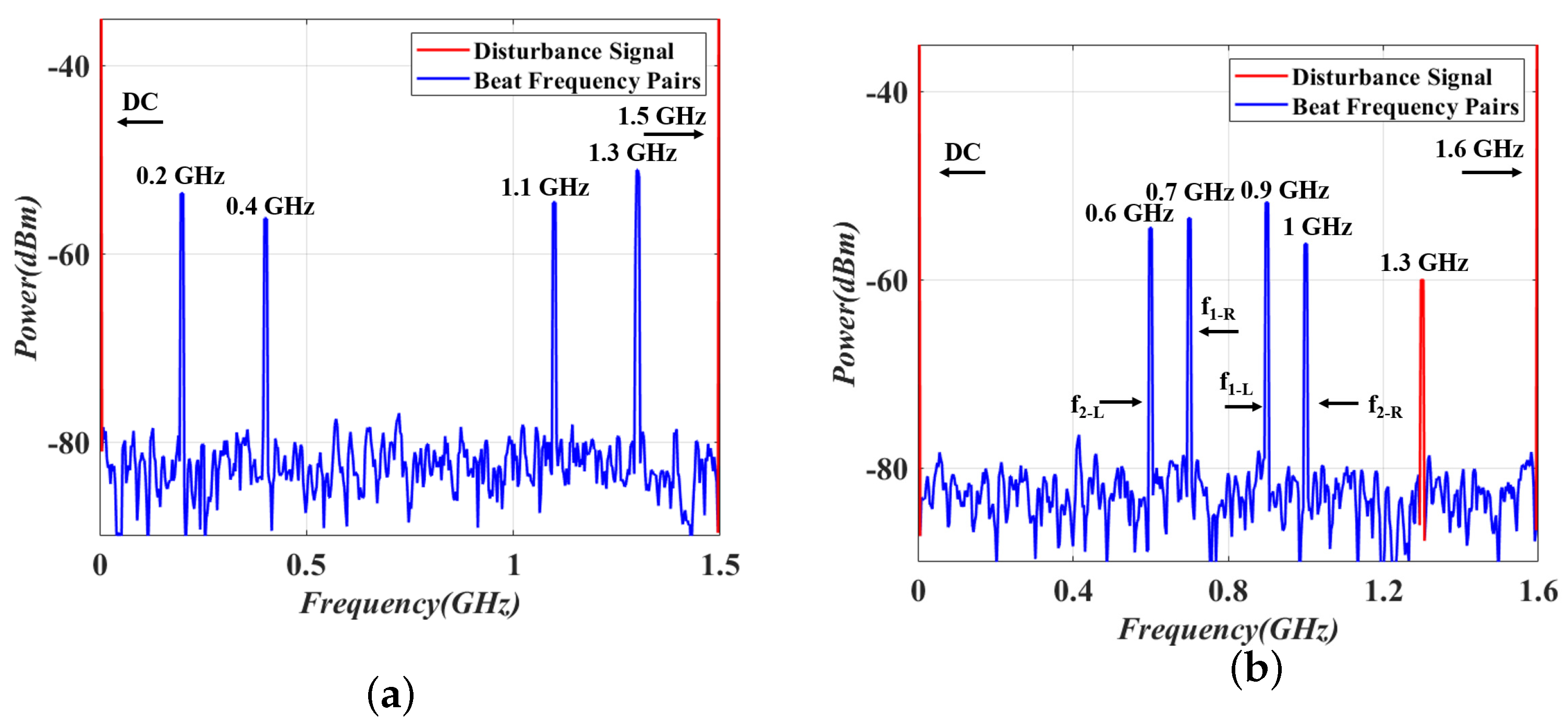
4.2. Frequency Ambiguity

In this part of the study, we discuss the frequency ambiguity of this system. As we have mentioned, the premises of acquiring accurate frequency estimations are: firstly, when extracting the spectrum information after PD, it should be limited to the interval $(0,f_s)$ due to the disturbance signal; second, it should be ensured that the incident RF signal is decomposed into two non-overlapping beat signal pairs whose sum is $f_s$. However, in some cases, the frequency measurement does not meet the above conditions, thus the frequency ambiguity problem occurs.

Table 2. The cases of frequency ambiguity in the proposed system.

Situation	Cases
Single-tone RF Measurement	$f=0$	$f=N\ast f_s$	$f=N\ast f_s/2$
Multi-tone RF Measurement	$f_1+f_2=N\ast f_s$ $f_1,f_2>0$	$\left|f_2-f_1\right|=N\ast f_s$ $f_1,f_2>0$	$\left|f_2-f_1\right|<f_s$ $\left|f_2-f_1\right|=f_{1,2-L,R}$

summarizes the frequency ambiguity that may occur in different scenarios. Specifically, in the case of a single-tone signal measurement, the unknown RF may not be identified in three situations, namely when its frequency is DC, it is the boundary frequency, or the signal is in the middle of the sub-channel. In the first two cases, the beat frequency of the RF signal is 0, and $f_s$ after decomposition, which is superimposed with the disturbance signal and makes it impossible to identify the input RF signal. In the last case, the frequency of the two signals after the beat is $f_s/2$, which makes it impossible to calculate the power ratio and thus identify the sub-channel to which the RF signal belongs.

When the multi-tone signal is measured, there are three kinds of frequency ambiguity. Suppose the incident signals are $f_1$ and $f_2$, and both $f_1$ and $f_2$ are greater than 0. The first case is when these two signals are symmetric with respect to $N\ast f_s$ or $N\ast f_s/2$, where N is a positive integer. In this case, the two generated beat signal pairs will overlap, which will affect the signal estimation. Secondly, if $f_1$ and $f_2$ are respectively located in two channels and their relative positions are the same, then $\left|f_2-f_1\right|=N\ast f_s$ is satisfied. The generated beat signal pairs will also overlap. The last one is the overlap of the disturbance and beat signals. This disturbance occurs when the interval between two unknown RF signals is less than $f_s$. Next, the beat frequency signal between $f_1$ and $f_2$ will be generated, as shown in Figure 6. Finally, if the disturbance signal overlaps with a signal of the beat frequency signal pair, the accuracy of the power ratio will be affected.

In fact, the frequency ambiguity problem can be solved by adjusting $f_s$. Changing $f_s$ means changing the channel interval, which will change the position of beat signal pair, thus breaking the symmetry or boundary problem of the original channel interval. In practice, two links with different comb spacing can be adopted due to the simple and compact structure of the system.

Figure 11 shows the results after receiving a two-tone signal, where $f_1=4.5$ GHz and $f_2=6.75$ GHz. Due to their frequency spacing being lager than the PD bandwidth, the result is similar with a single-tone signal measurement. These two signal frequencies are the boundary frequencies or in the middle of its sub-channel with a comb spacing of $1.5$ GHz. In this case, $f_1$ is decomposed into 0 and 1.5 GHz and $f_2$ is decomposed into 0.75 GHz, as shown in Figure 11a. The input signal cannot be identified effectively. By adjusting the comb spacing from 1.5 GHz to 1.6 GHz, the overlapping beat frequency pairs can be separated. Figure 11b illustrates the final result after PD when $f_s$ = 1.6 GHz. The powers of the beat frequency signals in 0.3 GHz, 0.35 GHz, 1.25 GHz and 1.3 GHz are −47.40 dBm, −50.90 dBm, −52.82 dBm and −43.85 dBm, respectively. The power ratios are calculated as 3.55 dB and 1.92 dB and the corresponding sub-channels are ch3 and ch5. In this way, the unknown RF signal is estimated as a two-tone signal, whose frequencies are 4.5 GHz and 6.75 GHz.

Figure 12 depicts the results after receiving a three-tone signal, where $f_1=2.1$ GHz, $f_2=3.9$ GHz and $f_3=5.4$ GHz. Among them, $f_1+f_2=4\ast f_s$ and $f_3-f_2=f_s$, which satisfy the first two cases under multi-tone signal measurement, as in Table 1. When the comb spacing is 1.5 GHz, the final result is shown in Figure 12a. It can be seen that $f_1$, $f_2$ and $f_3$ are all decomposed into 0.6 GHz and 0.9 GHz. This leads to a misjudgment in frequency estimation. After changing $f_s$ to 1.6 GHz, the overlapping beat frequency pairs appear in the spectrum as illustrated in Figure 12b. There are three beat frequency pairs, which meets the relationship of $f_{i-L}+f_{i_R}=f_s$, where $i=1$–3. According to their power ratios, the three-tone signal with frequencies $f_1=2.1$ GHz, $f_2=3.9$ GHz and $f_3=5.4$ GHz are identified. A disturbance signal of $f=1.5$ GHz is the beat frequency of $f_2=3.9$ GHz and $f_3=5.4$ GHz. This would not affect the result identification because it appears only by itself.

Finally, the last case under multi-tone signal measurement is investigated, where the disturbance between the multi-tone signals overlaps with the useful beat frequency pairs, which changes the value of the power ratio and further has an effect on the frequency identification. Figure 13 depicts the results after receiving a two-tone signal, where $f_1=7.3$ GHz and $f_2=8.6$ GHz. With a channel spacing of 1.5 GHz, $f_1$ is decomposed into 1.3 GHz and 0.2 GHz, and $f_2$ is decomposed into 1.1 GHz and 0.4 GHz. Moreover, the disturbance signal between $f_1$ and $f_2$ is also 1.3 GHz. Therefore, there are only four signals after PD, as shown in Figure 13a. In this case, the powers of 0.2 GHz and 1.3 GHz are −51.81 dBm and −49.00 dBm, respectively. The power ratio is 2.81 dB and its theoretical power ratio is 1.92 dB. By adjusting the comb spacing from 1.5 GHz to 1.6 GHz, the disturbance of 1.3 GHz is separated. The frequency pairs from 7.3 GHz are 0.7 GHz and 0.9 GHz. According to Figure 13b, their powers are −51.81 dBm and −49.89 dBm, respectively, and their power ratio is 1.92 dB. In this way, the frequency ambiguity problem is solved. It also should be mentioned that the frequencies of the disturbance signals in this case remain unchanged.

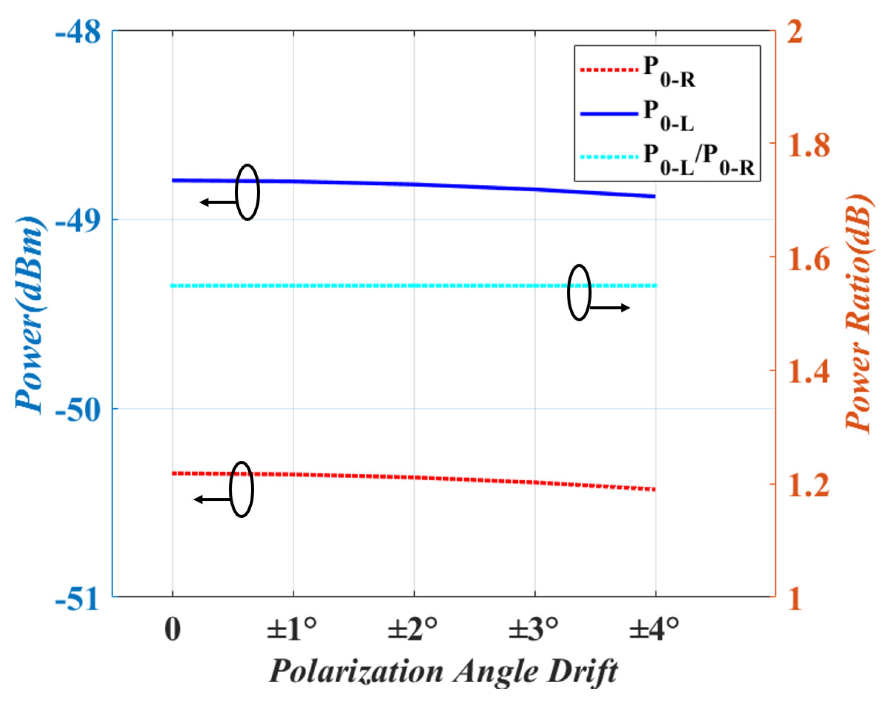
4.3. Polarization Angle Drift

In this part, we first discuss the effect of the polarizer angle drift on the system accuracy. The modulated signal and the non-flat OFC are combined via this 45-degree polarizer scheme. However, the beat signal power will be influenced by the polarization angle drift. To investigate it, a simulation based on different polarization angle drifts is carried out. Assuming the value of the angle drift is $\Delta \alpha$ = 0, 1, 2, 3 and 4 and the input signal frequency is $f_0=8.3$ GHz, the measured result is shown in Figure 14. As we can see, the powers of $f_{0-L}$ and $f_{0-R}$ decrease in a proportional way as the value of $\Delta \alpha$ increases. In this case, their power ratio remains constant, such that it can be concluded that the polarization angle drift only affect the beat signal power. Furthermore, the channel identification would be not influenced by the polarization angle drift.

Next, the MZM bias voltage of the PM-MZM will lead to the power variation of the center frequency. In the proposed scheme, the power ratio of ch1 is obviously larger than the others. This proves the system performance is not affected by the modulator bias drift and demonstrates good stability.

5. Conclusions

A photonics-based multiple microwave frequency measurement system has been presented. The system is designed to achieve a frequency down-conversion via a PM-MZM and a polarizer. It has the advantages of measuring multi-tone microwave signals with a simple and compact structure. Moreover, it has high measurement resolution and good stability, which is not affected by the polarizer or MZM bias drift. Additionally, free ambiguity operation is done to demonstrate the system performance. The trend of the simulated results is consistent with the trend of the theoretical results. Simulation results demonstrate a frequency measurement error of less than 2 MHz over 0.1–12 GHz.

The system resolution is due to the resolution of the post-processing devices and the bit rate of the sawtooth signal. According to Figure 7, there is a distinct power ratio difference in the first 8 channels. The resolution of the system among these channels is only dependent on the sampling rate of the ESA or the ADC and DSP devices, hence the high resolution can be achieved. The last 7 channels, have a power difference less than 0.2 dB. In this case, there is channel ambiguity in the background noise. The maximum estimated error is comparable to the rate of the sawtooth signal. Future works should investigate a new method to suppress the intermodulation interference in a multi-tone IFM system. It provides an important solution for a multi-tone IFM of an RF signal, which has applications in modern electronic warfare and wireless communication systems.

References

1. Spezio, A. Electronic warfare systems. IEEE Trans. Microw. Theory Tech. 2002, 50, 633–644. [Google Scholar] [CrossRef]
2. Capmany, J.; Mora, J.; Gasulla, I.; Sancho, J.; Lloret, J.; Sales, S. Microwave Photonic Signal Processing. J. Light. Technol. 2013, 31, 571–586. [Google Scholar] [CrossRef]
3. Yao, J.; Capmany, J. Microwave photonics. Sci. China-Inf. Sci. 2022, 65, 1–64. [Google Scholar] [CrossRef]
4. Li, J.; Pei, L.; Ning, T.; Zheng, J.; Li, Y.; He, R. Measurement of Instantaneous Microwave Frequency by Optical Power Monitoring Based on Polarization Interference. J. Light. Technol. 2020, 38, 2285–2291. [Google Scholar] [CrossRef]
5. Zhang, H.; Zheng, P.; Yang, H.; Hu, G.; Yun, B.; Cui, Y. A Microwave Frequency Measurement System Based on Si3N4 Ring-Assisted Mach-Zehnder Interferometer. IEEE Photonics J. 2020, 12, 7102213. [Google Scholar] [CrossRef]
6. Chen, H.; Huang, C.; Chan, E.H.W. Photonics-Based Instantaneous Microwave Frequency Measurement System with Improved Resolution and Robust Performance. IEEE Photonics J. 2022, 14, 5856008. [Google Scholar] [CrossRef]
7. Wang, S.; Wu, G.; Sun, Y.; Chen, J. Photonic compressive receiver for multiple microwave frequency measurement. Opt. Express 2019, 27, 25364–25374. [Google Scholar] [CrossRef] [PubMed]
8. Wang, X.; Zhou, F.; Gao, D.; Wei, Y.; Xiao, X.; Yu, S.; Dong, J.; Zhang, X. Wideband adaptive microwave frequency identification using an integrated silicon photonic scanning filter. Photonics Res. 2019, 7, 172–181. [Google Scholar] [CrossRef]
9. Xie, X.; Dai, Y.; Ji, Y.; Xu, K.; Li, Y.; Wu, J.; Lin, J. Broadband Photonic Radio-Frequency Channelization Based on a 39-GHz Optical Frequency Comb. IEEE Photonics Technol. Lett. 2012, 24, 661–663. [Google Scholar] [CrossRef]
10. Winnall, S.; Lindsay, A.; Austin, M.; Canning, J.; Mitchell, A. A microwave channelizer and spectroscope based on an integrated optical Bragg-grating Fabry-Perot and integrated hybrid fresnel lens system. IEEE Trans. Microw. Theory Tech. 2006, 54, 868–872. [Google Scholar] [CrossRef] [Green Version]
11. Wei, Y.; Wang, X.; Miao, Y.; Chen, J.; Wang, X.; Gong, C. Measurement and analysis of instantaneous microwave frequency based on an optical frequency comb. Appl. Opt. 2022, 61, 6834–6840. [Google Scholar] [CrossRef] [PubMed]
12. Liu, Y.; Guo, Y.; Wu, S. Frequency measurement of microwave signals in a wide frequency range based on an optical frequency comb and channelization method. Appl. Opt. 2022, 61, 3663–3670. [Google Scholar] [CrossRef] [PubMed]
13. Lu, X.; Pan, W.; Zou, X.; Bai, W.; Li, P.; Yan, L.; Teng, C. Wideband and Ambiguous-Free RF Channelizer Assisted Jointly by Spacing and Profile of Optical Frequency Comb. IEEE Photonics J. 2020, 12, 5500911. [Google Scholar] [CrossRef]
Figure 1. Schematic setup of the photonic MMFM system based on polarization interference and frequency converter. CW, continuous-wave laser; PC, polarization controller; RF, radio frequency; PM-MZM, polarization-multiplexing Mach–Zehnder modulator; PR, polarization rotator; PD, photodetector; and LPF, low-pass filter.
Electronics 12 00455 g001
Figure 2. ±1st-order optical-modulated signal spectrum after DSB.
Electronics 12 00455 g002
Figure 3. Waveform fo the periodic sawtooth wave signal.
Electronics 12 00455 g003
Figure 4. Spectrum diagram of the non-flat OFC.
Electronics 12 00455 g004
Figure 5. Spectrum diagram after a 45-degree polarizer.
Electronics 12 00455 g005
Figure 6. Spectrum diagram of the beat frequency signals after a PD and an LPF.
Electronics 12 00455 g006
Figure 7. Optical power ratio results of each channel.
Electronics 12 00455 g007
Figure 8. Measurement result using a single-tone signal, where f 0 = 8.3 GHz.
Electronics 12 00455 g008
Figure 9. Measurement result using a multi-tone signal, where f 1 = 1.9 GHz, f 2 = 3.3 GHz and f 3 = 10.7 GHz.
Electronics 12 00455 g009
Figure 10. Estimated error with different RF signals over 0.1–12 GHz.
Electronics 12 00455 g010
Figure 11. Receiving results for incoming signals at 4.5 and 6.75 GHz, where the comb spacing is (a) 1.5 GHz and (b) 1.6 GHz.
Electronics 12 00455 g011
Figure 12. Receiving results for incoming signals at 2.1, 3.9 and 5.4 GHz, where the comb spacing is (a) 1.5 GHz and (b) 1.6 GHz.
Electronics 12 00455 g012
Figure 13. Receiving results for incoming signals at 7.3 and 8.6 GHz, where the comb spacing is (a) 1.5 GHz and (b) 1.6 GHz.
Electronics 12 00455 g013
Figure 14. Powers of the beat signal pairs and their power ratios using different values for polarization angle drift in a single-tone signal, where f 0 = 8.3 GHz.
Electronics 12 00455 g014