Numerical Robustness Evaluation of Floating-Point Closed-Loop Control Based on Interval Analysis

Abstract

Power-electronics-based systems have penetrated into several critical sectors, such as the industry, power generation, energy transmission and distribution, and transportation. In this context, the system’s control, often implemented in real-time processing units, has to meet stringent requirements in terms of safety and repeatability. Given the growing complexity of the implemented algorithms, floating-point arithmetic is being increasingly adopted for high-performance systems. This paper proposes to assess the numerical stability of the control algorithms by means of an interval analysis. The case study of an electric drive is considered, given the wide adoption of such systems and the importance they hold for the safety of the applications. In particular, two different control strategies—the resonant control and the vector space decomposition—are examined, and a sensitivity analysis based on the proposed technique highlights the different characteristics of the two with respect to numerical stability. The proposed method shows how the resonant control is more robust to variations of the controller gain coefficients with respect to the numerical stability, which could make it the preferred choice for mission-critical electric drive control.

1. Introduction

The use of electric drives and static power conversion applications for mission-critical roles is rapidly expanding with the increasing push towards hybridization and electrification of the transportation sector. The main driver of this trend is the growing awareness of governments and international bodies for a large reduction in ${\mathrm{CO}}_2$ and ${\mathrm{NO}}_x$ emitted by aircraft [1]. In the aerospace field, in particular, there is great interest in the use of electrically driven fans as the main propulsion system of large commercial airliners, increasing overall system efficiency by enabling a more aerodynamically advantageous configuration, as shown in [2]. For these types of architecture to be viable, several advances are being actively researched by the scientific community. On the hardware side, the development trends towards high-power-density machines [3], the associated active rectifiers for medium-voltage DC (MVDC) power distribution [4], and scalable architectures for fault-tolerant machine and drive systems [5]. On the control system side, a lot of emphasis has been given to the development of high-performance fault-tolerant control systems that can manage highly redundant systems, both in terms of optimal postfault machine drive strategies [6], and fault-tolerant current control systems [7].

From an implementation perspective, the use of floating-point arithmetic is near ubiquitous in state-of-the-art control systems. This is due to their complexity, that makes the translation of these algorithms to fixed-point very hard, as well as to the availability of floating-point units (FPU) in most modern controllers. It is however, the use of floating-point arithmetic in mission-critical systems that poses some challenges, as this type of code can introduce numerical rounding errors, which can compound and interact in subtle and hard-to-identify ways [8]. The careful analysis of a floating-point control system implementation is consequently necessary to give strict bounds to these errors to ensure that their accumulation does not occur.

The only tools that can currently perform these types of studies are general-purpose static analysis suites, which, by evaluating an implementation at the source code level, can give guarantees on the magnitude of the errors introduced by floating-point calculations. In particular, SATIRE [9] is based on interval arithmetic and Fluctuat [10] employs weakly relational abstract domains. These analysis methods have some drawbacks that make them less than ideal for mission-critical power-electronics control applications. The first and by far biggest problem of the static approach is that the behaviour of the controlled portion of the system (also called the plant) has a very high degree of coupling with the controller, when operating in closed loop. Thus, an independent evaluation can result in very imprecise error bound estimation. While some tools can overcome this limitation, they require the external portion of the system to be modelled as a set of ordinary differential equation, which is not always practical, or even possible.

A second limitation of source-based static analysis tools is that their use restricts compilers to only use optimizations that are formally safe, in order not to invalidate the analysis results, forcing developers to make a choice between a suboptimal implementation or performing a manual optimization at the source code level, a tedious task that is very error-prone and greatly reduces overall code quality.

This paper proposes an interval-analysis-based technique that enables the evaluation of floating-point control algorithms’ implementations and overcomes the previously stated limitations. The use of a dynamic approach based on cosimulation, decouples the floating-point analysis from the plant model, allowing the use of a much wider selection of tools. Another advantage of the chosen approach is that it permits the use of potentially unsafe optimizations and even allows the strict quantification of the introduced error, enabling an informed trade-off choice between speed of execution and arithmetic precision.

Moreover, a figure of merit is introduced to globally evaluate the numerical robustness of the analysed code, allowing the use of many common engineering techniques, such as mathematical optimization or sensitivity analysis in this space. The paper is organized as follows. Section 2 presents an overview on interval arithmetic, the mathematical foundations upon which the proposed work is based. Then, in Section 3, the proposed analysis technique and robustness metrics are shown. Then, to showcase the potential of this technique in Section 4, a case study is used to demonstrate its potential impact in a real-world design scenario and conclusions are drawn in Section 5. Finally as appendicces all abbreviations and symbols are listed.

2. Interval- versus Floating-Point Arithmetic

Scientific computation is commonly implemented using floating-point numbers. These implementations have inherent inaccuracies, mainly due to round-off and truncation errors. Round-off errors arise because the continuum of real numbers is approximated by a finite set of finitely representable numbers. For instance, irrational numbers such as $\sqrt{2}$ cannot be represented exactly as finite-precision floating-point numbers. Even a rational number such as one-third cannot be represented as a binary floating-point number. Truncation error arises when an infinite mathematical process is approximated using a finite initial segment. For example, in the numerical computation of the transcendental function $exp\left(x\right)={\sum }_{n=0}^{\infty }{x}^n/n!$, the infinite series is truncated at a (sufficiently large) index M, and the value ${exp}_M\left(x\right)={\sum }_{n=0}^M{x}^n/n!$ is returned as a sufficiently close approximation of the true value of ${\mathrm{e}}^x$.

A full error analysis of floating-point computations may be carried out in some cases. Examples include basic arithmetic operations, the evaluation of polynomials, matrix inversion, QR factorization [11], and the solution of the 1D wave equation [12], to mention a few. In general, however, a full error analysis of floating-point computations is a complicated task, and the computations may be deceptively unstable, even when the operations involved are rather simple [11,13,14,15]. An effective alternative is developing algorithms which are correct by construction, that is, they do not require a separate error analysis. Numerical methods that incorporate explicit and strict error evaluations, referred to as validated numerics [16], offer a sound alternative of this kind, where results are provided with absolute guarantees of correctness. Interval arithmetic [17], in particular, is a common framework for developing validated algorithms.

2.1. Interval Arithmetic

In contrast with the classical arithmetic which is performed over individual numbers, interval arithmetic is performed over sets of numbers. As the result of each operation is also a set, it is possible to incorporate all the possible errors (such as round-off and truncations errors) into the result. Interval arithmetic provides a powerful method for obtaining guaranteed bounds on errors that arise from various sources, including floating-point errors and imprecision in physical measurements.

As an example, assume that the result of the measurement of a quantity x is $x_0$, and the measuring equipment has a precision of $\delta$. Then, it is reasonable to represent the uncertain value of x with the interval $[x_0-\delta ,x_0+\delta ]$. The central task in interval arithmetic is to bound the uncertainties as they propagate through the computation steps. For instance, if it is known that $x\in [x_1,x_2]$ and $y\in [y_1,y_2]$, then, clearly, $x+y\in [x_1+y_1,x_2+y_2]$ and $x-y\in [x_1-y_2,x_2-y_1]$. If $x_1,y_1\ge 0$, then $xy\in [x_1{y}_1,x_2{y}_2]$. However, multiplication is slightly more complicated when the intervals contain negative values. Thus, in general:

$$xy\in [min\left\{x_1{y}_1,x_1{y}_2,x_2{y}_1,x_2{y}_2\right\},max\left\{x_1{y}_1,x_1{y}_2,x_2{y}_1,x_2{y}_2\right\}].$$

Interval division is even more complicated as in the case where $0\in [y_1,y_2]$ produces unbounded intervals.

Let ${\mathbb{R}}_{\infty }:=\mathbb{R}\cup \left\{-\infty ,+\infty \right\}$ denote the set of extended real numbers, and let $\mathbb{I}{\mathbb{R}}_{\infty }$ denote the set of intervals over the extended real line, that is, $\mathbb{I}{\mathbb{R}}_{\infty }:=\{[a,b]\mid -\infty \le a\le b\le +\infty \}$. In general, for any function $f:{\mathbb{R}}_{\infty }\to {\mathbb{R}}_{\infty }$, a map $\widehat{f}:\mathbb{I}{\mathbb{R}}_{\infty }\to \mathbb{I}{\mathbb{R}}_{\infty }$ is said to be an interval approximation of f if, for any given interval $[a,b]$, the following relation holds:

$$f\left([a,b]\right):=\left\{f\left(x\right)x\in [a,b]\right\}\subseteq \widehat{f}\left([a,b]\right).$$

(1)

In simple terms, $\widehat{f}\left([a,b]\right)$ bounds the range of values that f takes over the interval $[a,b]$. Note that the relation in (1) is a subset relation and not an equality. The reason is that, in general, enforcing equality is either too costly or practically impossible, for instance, when the endpoints are floating-point numbers. Of course, tighter interval approximations are preferred because of the higher accuracy of the results that they provide. Obtaining tight interval approximations of functions such as sin, cos and exp requires a careful analysis, which is outside the scope of the current article. For more details, the reader may refer to [17,18].

The standard IEEE Std 1788-2015 [19] for interval arithmetic was approved in 2015, and many libraries exist for interval computation in various languages. Common interval libraries either use fixed-precision or arbitrary-precision floating-point endpoints for the representation of intervals. To account for all the possible errors, outward rounding must be implemented, that is, when computing interval results, the left-end point must be rounded towards $-\infty$ and the right endpoint must be rounded towards $+\infty$. In the current work, the arbitrary-precision library MPFI [20] was used. Specifically, the C++ Boost library implementation was chosen, which provides a wrapper around the original MPFI types [21].

On the theoretical side, interval arithmetic has a firm foundation in domain theory [22], and it has proven to be a useful tool in fundamental research. In fact, interval arithmetic gained further prominence when it was used to prove that the Lorenz attractor was a strange attractor, thereby solving Smale’s fourteenth problem [23]. Nevertheless, there are pitfalls in using interval arithmetic as well.

2.2. Sources of Inaccuracy in Interval Computations

Inaccuracies enter into interval computations for a variety of reasons, with the following ones being the most relevant to the current article:

Finite representations: If any of the endpoints of an interval is not representable as a floating-point number, then the interval must be rounded outwards. For instance, let $\mathrm{e}$ be the Euler number. As $\mathrm{e}$ is an irrational number, it does not have a finite binary expansion. Thus, in MPFI, when the precision is set to 10, the result of $exp\left(\right[1,1\left]\right)$ is given as $[2.718281828,2.718281829]$. Furthermore, as the precision of the endpoints of each interval must be set first, an inaccuracy is incurred even on simpler computations. For example, if the bit size is set to n, then the result of $[0,0]+[-2^{-2n},2^{-2n}]$ must be rounded outwards to $[-2^{-n},2^{-n}]$. This source of inaccuracy is inevitable and, to a large extent, harmless. The reason is that a higher accuracy may be obtained by simply increasing the bit size of the representation of the endpoints.

Dependency: By default, interval computations do not take into account any dependencies between parameters. For instance, assume that $x\in [0,1]$. Applying interval subtraction results in $(x-x)\in [-1,1]$, which is a significant overestimation as the true value is $x-x=0$. In some cases, inaccuracies arising from the dependency problem can be reduced by using a hybrid symbolic–interval method [24].

Wrapping effect: Whenever a set which is not a hyperbox is overapproximated by a bounding hyperbox, some accuracy is lost. This source of inaccuracy in interval arithmetic is referred to as the wrapping effect [25]. An example is depicted in Figure 1, in which the dashed square represents $(x,y)=\left(\right[-1,1],[-1,1\left]\right)$. Let

$$R_{\theta }:=\left[\begin{array}{cc}cos\left(\theta \right)& -sin\left(\theta \right)\\ sin\left(\theta \right)& cos\left(\theta \right)\end{array}\right]$$

be the rotation map around the origin through the angle $\theta$. The result of $R_{\pi /4}(x,y)$ is the square (drawn in blue) whose sides are not parallel to the x and y axes. Hence, it must be bounded by a larger box, which is the outermost square drawn in black.

As a result, interval computations are prone to overestimations which, at times, are too conservative, especially when long sequences of computations are performed. Nonetheless, even when the bounds are wide, interval computations can provide valuable insight into the sensitivity of computation processes with respect to designated parameters, as shall be demonstrated in what follows.

3. Verification of Closed-Loop Floating-Point Core

The aim of the analysis technique presented in this paper is the definition of a figure of merit, the robustness performance indicator (abbreviated to RPI) to allow the comparison of numerical robustness of various control techniques and their floating-point implementations. This type of evaluation system is a delicate balancing act of many different aspects that make this operation fairly hard, especially when applied to closed-loop processes where it is not possible to define a clear line of demarcation between the dynamics of the controller and the controlled system. Static-analysis-based approaches, while simple to apply and requiring minimal changes to existing code, need the inclusion of the mathematical model of the controlled plant, as it has a deep influence over the controller behaviour which is, unfortunately, very challenging, as the switching behaviour of power electronic converters can be highly nonlinear. For the aforementioned reasons, the technique proposed in this paper is based on a dynamic analysis, as the study of the system while in operation completely bypasses the issue.

The core robustness metric that can be derived from an interval analysis is the width of the confidence interval within which a specific value is guaranteed to lie, having taken into account all uncertainties. This value, however, is not guaranteed to be monotonically increasing. A factor that significantly complicates the comparison of different implementations or algorithms is that these local minimums and maximums in the confidence interval width do not occur at the same time, but rather depend on how the whole system evolves, making the result of any comparison effectively dependent on the choice of instant at which it is performed. To make the RPI immune to this issue, it is defined as follows:

$$RPI={\int }_0^{T_{SIM}}\sum _{x=1}^N{E}_{W_x\left(t\right)}dt,$$

(2)

where $E_{W_x\left(t\right)}$ is the confidence interval width for the xth quantity of interest. The use of the integral over the whole duration of a simulation (from start to $T_{SIM}$) allows the RPI to take into account the complete history of the error width for the relevant period, enabling comparisons between differing implementations, provided that the length of the examined period is kept constant.

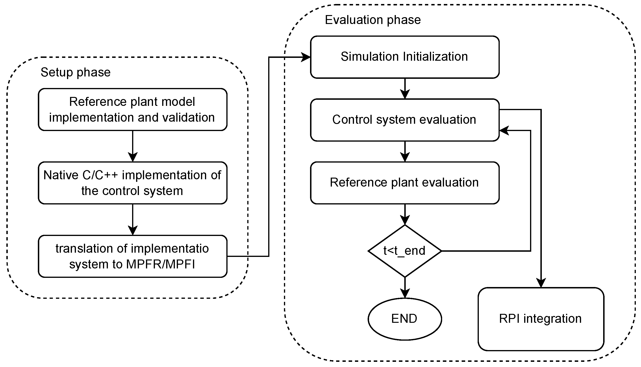
A diagram of the complete workflow for the proposed robustness analysis is shown in Figure 2. It can be broken down in two distinct phases. The first one, the study setup, is only performed once for a given control system and involves the implementation of all the base building blocks that are needed for the simulation and to calculate the RPI. The second phase, the system evaluation, consists in repeated simulations where the numerical robustness of the target system is evaluated for various parameter values and operating conditions.

3.1. Setup Phase

In this preparatory phase, the instrumented cosimulation models needed for the proposed analysis technique are developed and validated. The first step of this phase involves the creation of a reference plant model that will be used throughout the whole analysis. This needs to be sufficiently detailed to accurately capture the system behaviour, while being as computationally efficient as possible to enable the use of this technique with optimizations, sensitivity analyses and other engineering methods that involve repeated system evaluations. Upon completion, the model should be experimentally validated, to ensure that it correctly captures the behaviour of the examined system and that an acceptable degree of modelling accuracy has been achieved, meaning only acceptably small errors between predicted and measured value of the studied variables. This is crucial to ensure the applicability of the results to real-world scenarios. Once the model is ready, the second step of the process calls for the C/C++ implementation of the target control system or the adaptation of an existing implementation to work with the simulator of choice. In a first phase, the use of native floating-point types is advised to eliminate a potential source of inconsistencies, helping to achieve a well-rounded, stable, and fast simulation. Once this is ready, the final step of the setup phase involves swapping the control system implementation with one that makes use of the MPFI types for the interval analysis. This, in addition to the control system evaluation, also has to convert the controller inputs to intervals, taking into account the eventual sensor noise and precision, and converting the outputs to regular floating-point values that will be passed to the system model.

3.2. Evaluation Phase

The evaluation phase is at the core of the proposed analysis technique; it is in this phase that the instrumented simulation developed during setup is actually run to evaluate the robustness of the developed model with respect to various operating conditions, added uncertainties, etc. In this phase, the simulation is repeatedly evaluated with different combinations of parameters to investigate how the RPI evolves. From an operative standpoint, this phase consists of a regular control level simulation where, after the initialization is complete, the control system and reference plant model are evaluated repeatedly in a loop. For each time step, the confidence interval for the studied quantities (i.e., controller outputs, state variables, etc.) are calculated and then numerically integrated to update the overall RPI value. The length of the operating period to be simulated is chosen to be only as long as necessary to be relevant with respect to the studied system dynamics, to reduce the computational cost as much as possible.

4. Case Study

This section presents a real-world case study, where the analysis technique presented previously is applied to a concrete power electronics control problem. This highlights the usefulness of the proposed robustness index and how this can be used by both hardware designers and control system engineers to quickly assess the impact of their choice over the numerical robustness of the control system implementation.

4.1. System and Control Architecture

The target system, whose schematic representation is shown in Figure 3, consisted of a six-phase asymmetric permanent magnet synchronous machine (PMSM), whose stator was composed by two star-connected three-phase winding sets with a radial shift of $30{}^{\circ }$ between them. The current in each phase was managed by a separate node consisting of a half-bridge power section, with the relative support circuitry. The control system was implemented on a single centralized controller, which was linked by a digital communication protocol with each single-phase driving cell.

From a control system perspective, two different techniques were compared. The first one was based on the traditional vector space decomposition (VSD) and used standard proportional–integral (PI) regulators relying on a change from a static to rotating reference frame to avoid tracking a sinusoidal reference, as shown in Figure 4a. The second control methodology examined in this comparison was the direct current control, presented in [5] and shown in Figure 4b, where the current flowing in each phase is controlled directly in the static reference frame through the use of a proportional, integral, and resonant (PIR) controller, which is able to track a sinusoidal reference with arbitrary frequency. This technique has the advantage of completely decoupling the control for each phase, potentially allowing distributed current control, improving the modularity and fault tolerance of the entire system.

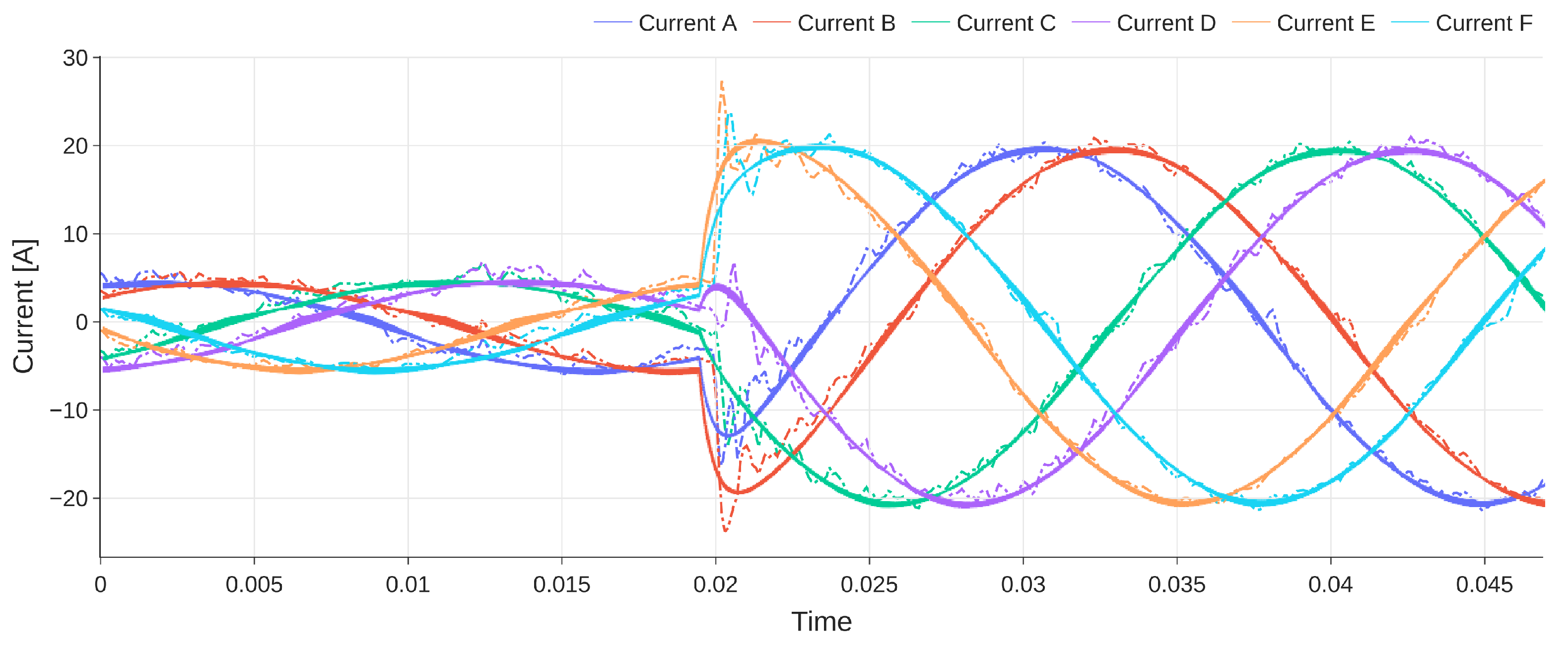
The machine and inverter models, whose main parameters are shown in

Table 1. Parameters of the studied system.

Parameter	Value
DC-link voltage	$270 \mathrm{V}$
Motor rated power	$18 \mathrm{k}\mathrm{W}$
Stator inductance	$125 \mathsf{\mu }\mathrm{H}$
Stator resistance	$8.5 \mathrm{m}\Omega$
Switching frequency	$60 \mathrm{k}\mathrm{Hz}$
Pole pairs	4

, were constructed in the PLECS environment and experimentally validated against the data collected in [5]. This is demonstrated in Figure 5, which compares the phase current waveforms captured during an experiment with their simulated analogues. The performed load-step test consisted of a sudden change in the current setpoint, that allowed the verification of a good match between the two sets of waveforms, both in the steady state and during transients. This gave confidence that the numerical model used in this work was in strong agreement with the prototype system result and could be therefore adopted for the algorithm evaluation.

The control system for both studied architectures was initially implemented in C with native single floating-point arithmetic, targeting the femtoCore processor [26], and then converted to use MPFI types. A preliminary step for the subsequent analyses was the individuation of the various design and operating parameters whose impact on numerical stability needed to be evaluated, as shown in

Table 2. Studied operating parameters.

Resonant Control	VSD Control
Proportional gain	Proportional gain for $\alpha \beta$ controllers
Resonant gain	Integral gain for $\alpha \beta$ controllers
Damping	Proportional gain for $xy$ and 0 controllers
Current sensor error	Integral gain for $xy$ and 0 controllers
Frequency sensor error	Current sensor error
Speed	Angle sensor error
	Speed

.

The developed model could, at this point, be used to evaluate, through the procedure outlined in Section 3, the system behaviour with respect to the numerical robustness of the controller output. The first step was a global sensitivity analysis, a technique that uses a representative sample of the parameters’ input space to quickly evaluate how sensitive the controller output’s numerical stability is to the variation of each single parameter, through a variance analysis. This step reduced the number of relevant parameters, enabling the use of a more powerful and computationally intensive Monte Carlo statistical analysis, to exactly determine the distribution of RPI values within the defined range of inputs.

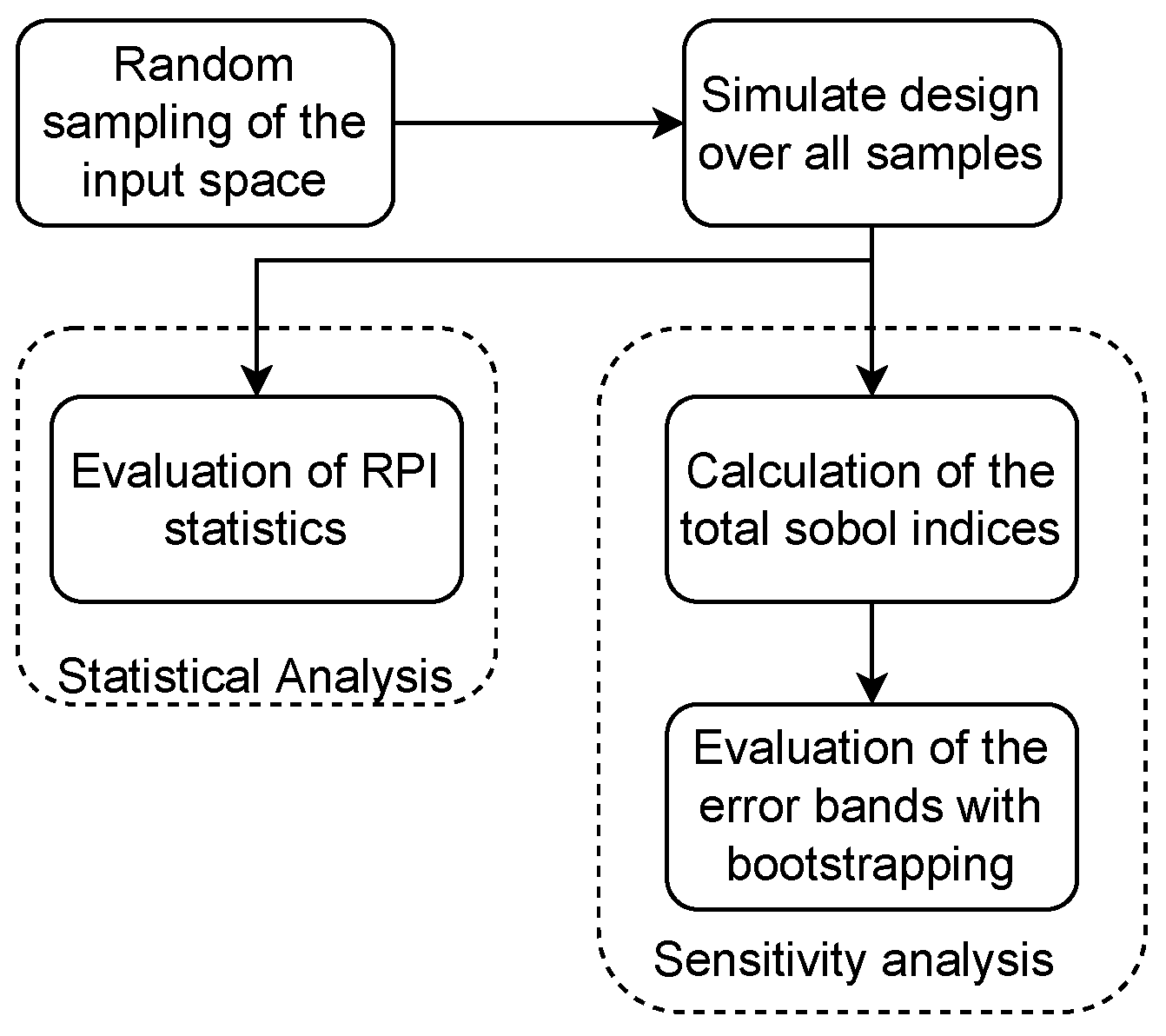
First, a sensitivity analysis was conducted to evaluate which of the parameters had the highest impact, then a more in-depth statistical analysis was performed to directly compare the two control techniques. Figure 6 shows as a flowchart the analysis process used in this case study.

4.2. Sensitivity Analysis

Given the multitude of parameters that can affect the numerical stability of a real-world control system implementation, a sensitivity analysis was a necessary step to estimate the relative impact of each of them on the RPI, reducing both computational and analytical effort needed for more in-depth analyses that could be run on the most important factors only. The simplest and most intuitive methodologies that are often used for this task belong to the class of one-at-a-time (OAT), also known as local, methods. These involve changing a single parameter for each experiment while the nominal value is used for all others. A fundamental problem of these type of methods is that they are only applicable to linear models, as their coverage of the input space decreases as the number of parameters increases, as shown in [27]. When working with complex problems, such as the numerical stability of control systems, a variance-based global sensitivity analysis method [28] should be used. These methods have the advantage of being capable of working with models that present nonlinearities and some interaction between inputs.

From an operative perspective, the initial step required the generation of two groups of completely uncorrelated points, sampled from the entire model input space. To do this, the Sobol low-discrepancy sequence [29] was used, as it greatly reduced the number of model evaluations needed by sampling the input spaces in a more uniform fashion, as opposed to a pseudorandom sampling. The simulation was then run, obtaining as an output an RPI for each point. These data were then used to estimate the total Sobol sensitivity index $S_{Ti}$, defined as:

$$S_{Ti}=\frac{E_{{\mathbf{X}}_{\sim i}}\left(V_{X_i}(Y\mid {\mathbf{X}}_{\sim i})\right)}{V\left(Y\right)}$$

(3)

where $\mathbf{Y}$ denotes the random variable associated with the model output, ${\mathbf{X}}_i$ the one connected to the examined parameter while ${\mathbf{X}}_{\sim i}$ indicates the random variable of all other uncertain parameters. Finally, following the conventional notation, $\mathbf{E}\left(\right)$ indicates the average value and $\mathbf{V}\left(\right)$ the variance. The method presented in [30] was used to estimate these the indicators as a direct calculation through simple Monte Carlo simulations was computationally prohibitively expensive. The bootstrapping technique [31] was used to obtain an estimate of the confidence interval for the sensitivity index of each parameter.

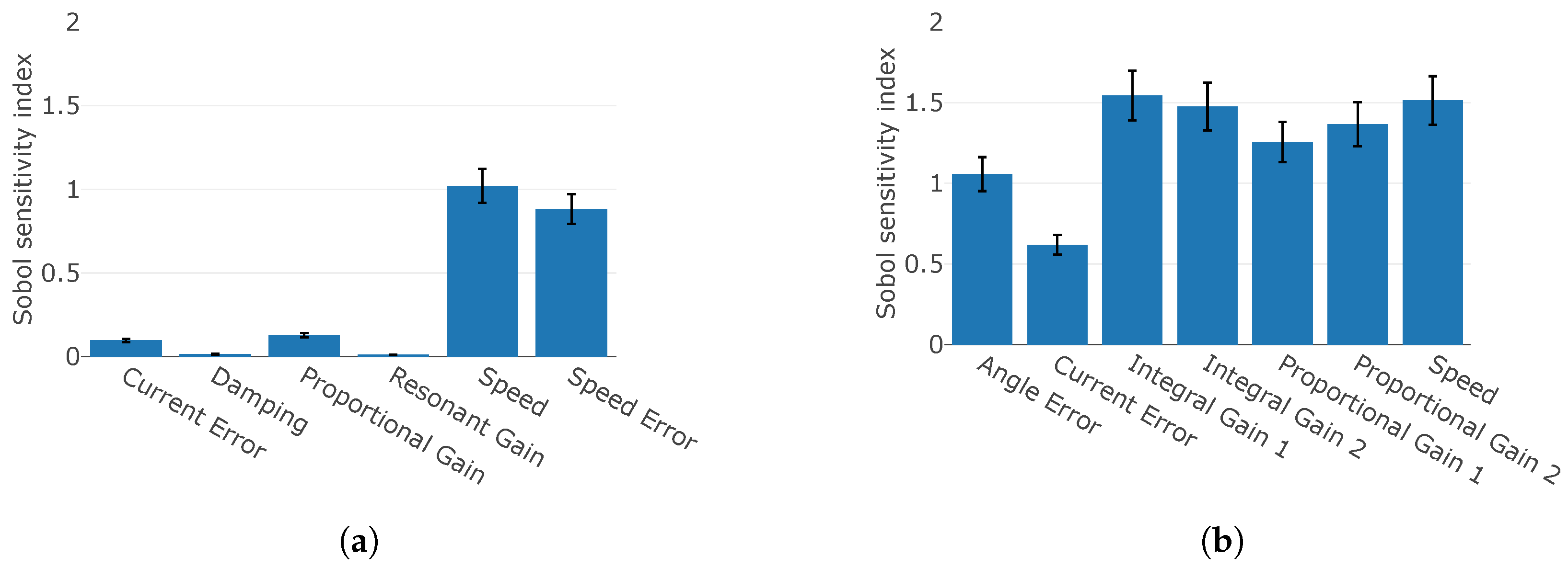
The results of the analysis for the resonant control are shown in Figure 7a. The first observation that can be drawn from these data is that the numerical robustness of the resonant controller, in its simplest implementation, was deeply affected by the operating speed, as was its performance [32]. Naturally, another factor with a large impact was the speed sensor error, as it interacted with the speed itself. A more surprising conclusion was the relatively low impact of the controller’s tuning parameters to the numerical robustness of the overall control system, especially with respect to the resonant element. This result uncovered a dependence between the speed-sensing performance and the numerical robustness of the control, thus a high-performance direct speed-sensing technique should be used, as opposed to the more indirect sensing strategy, relying on the derivative of the angle measurement.

The situation was fairly different when examining VSD control, whose results are shown in Figure 7b. The controller tuning parameters had a relatively large and even impact on the numerical robustness of the control system, along with the speed. Surprisingly, the sensors’ accuracy had a lower impact, for both current and angle measurements. This is positive for low-end applications, where cheaper sensing strategies can be used effectively; however, it is not ideal for mission-critical systems, where numerical robustness and performance consistency is more important than sensor cost.

Overall, it can be concluded that for mission-critical systems, resonant control is the better option, from a numerical robustness perspective, as it exhibits a much lower sensitivity to controller parameters, affording much more freedom during tuning. On the other hand, the current sensor choice is also much more critical for the VSD method as it had a fairly large effect on the RPI as opposed to resonant techniques.

4.3. Statistical Analysis

Given the large number of parameters and operating conditions that control system implementations are supposed to operate in, only statistical approaches can offer a meaningful numerical stability analysis, allowing direct comparisons. The starting point for this analysis was a set of input samples covering the entire design space. It was defined by current and angle/speed-sensing errors and constructed with the same low-discrepancy sequence that was also used in the sensitivity analysis. The model was then evaluated at each sample point, collecting the resulting RPI. Figure 8 shows the distribution of RPI indices across the whole input space. It should be noticed that given the large range of variability in index values, the base 10 logarithm was used to better highlight the histogram shapes. These show that both techniques achieved a comparable RPI (${10}^6$), making them largely equivalent in term of worst-case robustness performance. Globally, however, the distributions had very different shapes, with resonant control having a uniform distribution over the entire range of RPI values, whereas VSD control showed a definite peak with a negatively skewed Gaussian distribution. This is well reflected in the mean and median values shown in

Table 3. RPI analysis results.

Technique	Mean RPI	Median RPI	Variance
Resonant	$22.94\times {10}^3$	$283.84$	$5.90\times {10}^9$
VSD	$129.92\times {10}^3$	$105.83\times {10}^3$	$9.03\times {10}^9$

.

5. Conclusions

This paper introduced a novel technique for the evaluation of the numerical robustness of floating-point control systems that widened the applicability of formal verification techniques. Moreover, the cosimulation approach greatly simplified the integration of the numerical robustness quantification with respect to other more general-purpose techniques. This enabled a case study that highlighted significant differences in the numerical robustness of two widely used current control methodologies and demonstrated a significant advantage of resonant control over vector space decomposition within this area.

References

1. Directorate-General for Mobility and Transport (European Commission); Directorate-General for Research and Innovation (European Commission). Flightpath 2050: Europe’s Vision for Aviation: Maintaining Global Leadership and Serving Society’s Needs; Publications Office: Geneva, Switzerland, 2011. [Google Scholar] [CrossRef]
2. Gibson, A.; Hall, D.; Waters, M.; Masson, P.; Schiltgen, B.; Foster, T.; Keith, J. The Potential and Challenge of TurboElectric Propulsion for Subsonic Transport Aircraft. In Proceedings of the 48th AIAA Aerospace Sciences Meeting Including the New Horizons Forum and Aerospace Exposition, Orlando, FL, USA, 4–7 January 2010. [Google Scholar] [CrossRef]
3. Golovanov, D.; Gerada, D.; Sala, G.; Degano, M.; Trentin, A.; Connor, P.H.; Xu, Z.; Rocca, A.L.; Galassini, A.; Tarisciotti, L.; et al. 4-MW Class High-Power-Density Generator for Future Hybrid-Electric Aircraft. IEEE Trans. Transp. Electrif. 2021, 7, 2952–2964. [Google Scholar] [CrossRef]
4. Trentin, A.; Sala, G.; Tarisciotti, L.; Galassini, A.; Degano, M.; Connor, P.H.; Golovanov, D.; Gerada, D.; Xu, Z.; La Rocca, A.; et al. Research and Realization of High-Power Medium-Voltage Active Rectifier Concepts for Future Hybrid-Electric Aircraft Generation. IEEE Trans. Ind. Electron. 2021, 68, 11684–11695. [Google Scholar] [CrossRef]
5. Savi, F.; Barater, D.; Buticchi, G.; Gerada, C.; Wheeler, P. A Scalable System Architecture for High-Performance Fault Tolerant Machine Drives. IEEE Open J. Ind. Electron. Soc. 2021, 2, 428–440. [Google Scholar] [CrossRef]
6. Bianchi, N.; Bolognani, S.; Dai Pre, M. Strategies for the Fault-Tolerant Current Control of a Five-Phase Permanent-Magnet Motor. IEEE Trans. Ind. Appl. 2007, 43, 960–970. [Google Scholar] [CrossRef]
7. Kiselev, A.; Catuogno, G.R.; Kuznietsov, A.; Leidhold, R. Finite-Control-Set MPC for Open-Phase Fault-Tolerant Control of PM Synchronous Motor Drives. IEEE Trans. Ind. Electron. 2020, 67, 4444–4452. [Google Scholar] [CrossRef]
8. Sanchez-Stern, A.; Panchekha, P.; Lerner, S.; Tatlock, Z. Finding Root Causes of Floating Point Error. SIGPLAN Not. 2018, 53, 256–269. [Google Scholar] [CrossRef]
9. Das, A.; Briggs, I.; Gopalakrishnan, G.; Krishnamoorthy, S.; Panchekha, P. Scalable yet Rigorous Floating-Point Error Analysis. In Proceedings of the SC20: International Conference for High Performance Computing, Networking, Storage and Analysis, Atlanta, GA, USA, 9–19 November 2020; pp. 1–14. [Google Scholar] [CrossRef]
10. Delmas, D.; Goubault, E.; Putot, S.; Souyris, J.; Tekkal, K.; Védrine, F. Towards an Industrial Use of FLUCTUAT on Safety-Critical Avionics Software. In Formal Methods for Industrial Critical Systems; Springer: Berlin/Heidelberg, Germany, 2009; pp. 53–69. [Google Scholar]
11. Higham, N.J. Accuracy and Stability of Numerical Algorithms, 2nd ed.; Society for Industrial and Applied Mathematics: Philadelphia, PA, USA, 2002. [Google Scholar]
12. Boldo, S.; Melquiond, G. Computer Arithmetic and Formal Proofs: Verifying Floating-Point Algorithms with the Coq System; Elsevier: Amsterdam, The Netherlands, 2017. [Google Scholar]
13. Muller, J.M. Arithmétique des Ordinateurs; Masson: Paris, France, 1989. [Google Scholar]
14. Muller, J.M. Ordinateurs en quête d’arithmétique. La Rech. 1995, 26, 772–777. [Google Scholar]
15. Ménissier-Morain, V. Arbitrary precision real arithmetic: Design and algorithms. J. Log. Algebr. Program. 2005, 64, 13–39. [Google Scholar] [CrossRef]
16. Tucker, W. Validated Numerics: A Short Introduction to Rigorous Computations; Princeton University Press: Princeton, NJ, USA, 2011. [Google Scholar]
17. Moore, R.E.; Kearfott, R.B.; Cloud, M.J. Introduction to Interval Analysis; Society for Industrial and Applied Mathematics: Philadelphia, PA, USA, 2009. [Google Scholar]
18. Hansen, E.; Walster, G.W. Global Optimization Using Interval Analysis; Pure and Applied Mathematics Series; Marcel Dekker: New York, NY, USA, 2004. [Google Scholar]
19. IEEE Std 1788-2015; IEEE Standard for Interval Arithmetic. IEEE SA: Piscataway, NJ, USA, 2015. Available online: https://standards.ieee.org/ieee/1788/4431/ (accessed on 29 December 2022).
20. Revol, N.; Rouillier, F. Motivations for an Arbitrary Precision Interval Arithmetic and the MPFI Library. Reliab. Comput. 2005, 11, 275–290. [Google Scholar] [CrossRef] [Green Version]
21. MPFI Boost Multiprecision Library. Available online: https://www.boost.org/doc/libs/1_76_0/libs/multiprecision/doc/html/boost_multiprecision/tut/interval/mpfi.html (accessed on 19 December 2022).
22. Duracz, J.; Farjudian, A.; Konečný, M.; Taha, W. Function Interval Arithmetic. In Mathematical Software—ICMS 2014; Hong, H., Yap, C., Eds.; Lecture Notes in Computer Science; Springer: Berlin/Heidelberg, Germany, 2014; Volume 8592, pp. 677–684. [Google Scholar]
23. Tucker, W. A rigorous ODE solver and Smale’s 14th problem. Found. Comput. Math. 2002, 2, 53–117. [Google Scholar] [CrossRef] [Green Version]
24. Wang, S.; Pei, K.; Whitehouse, J.; Yang, J.; Jana, S. Formal Security Analysis of Neural Networks Using Symbolic Intervals. In Proceedings of the 27th USENIX Conference on Security Symposium (SEC’18), Baltimore, MD, USA, 15–17 August 2018; pp. 1599–1614. [Google Scholar]
25. Neumaier, A. The Wrapping Effect, Ellipsoid Arithmetic, Stability and Confidence Regions. In Validation Numerics: Theory and Applications; Albrecht, R., Alefeld, G., Stetter, H.J., Eds.; Springer: Vienna, Austria, 1993; pp. 175–190. [Google Scholar] [CrossRef] [Green Version]
26. Savi, F.; Harikumaran, J.; Barater, D.; Buticchi, G.; Gerada, C.; Wheeler, P. Femtocore: An Application Specific Processor for Vertically Integrated High Performance Real-Time Controls. IEEE Open J. Ind. Electron. Soc. 2021, 2, 479–488. [Google Scholar] [CrossRef]
27. Saltelli, A.; Aleksankina, K.; Becker, W.; Fennell, P.; Ferretti, F.; Holst, N.; Li, S.; Wu, Q. Why so many published sensitivity analyses are false: A systematic review of sensitivity analysis practices. Environ. Model. Softw. 2019, 114, 29–39. [Google Scholar] [CrossRef]
28. Sobol, I. Global sensitivity indices for nonlinear mathematical models and their Monte Carlo estimates. Math. Comput. Simul. 2001, 55, 271–280. [Google Scholar] [CrossRef]
29. Sobol, I. On the distribution of points in a cube and the approximate evaluation of integrals. USSR Comput. Math. Math. Phys. 1967, 7, 86–112. [Google Scholar] [CrossRef]
30. Hervé Monod, C.N.; Makowski, D. Uncertainty and Sensitivity Analysis for Crop Models; Elsevier: Amsterdam, The Netherlands, 2006. [Google Scholar]
31. Davison, A.C.; Hinkley, D.V. Bootstrap Methods and Their Application; Cambridge Series in Statistical and Probabilistic Mathematics; Cambridge University Press: Cambridge, UK, 1997. [Google Scholar] [CrossRef]
32. Yepes, A.G.; Freijedo, F.D.; Doval-Gandoy, J.; López, O.; Malvar, J.; Fernandez-Comesaña, P. Effects of Discretization Methods on the Performance of Resonant Controllers. IEEE Trans. Power Electron. 2010, 25, 1692–1712. [Google Scholar] [CrossRef]
Figure 1. Wrapping effect.
Electronics 12 00390 g001
Figure 2. Flow diagram of the proposed numerical robustness analysis technique.
Electronics 12 00390 g002
Figure 3. Diagram of the hardware configuration used in the case study.
Electronics 12 00390 g003
Figure 4. Overview of the examined control techniques: (a) vector space decomposition (VSD) and (b) resonant current control.
Electronics 12 00390 g004
Figure 5. Comparison between experimental data (dashed line) and simulation results (solid line).
Electronics 12 00390 g005
Figure 6. Flow diagram of the analyses used performed in this case study.
Electronics 12 00390 g006
Figure 7. Results of the case study: (a) sensitivity analysis for resonant control, (b) sensitivity analysis for VSD control.
Electronics 12 00390 g007
Figure 8. Statistical comparison in RPI distribution between the two strategies.
Electronics 12 00390 g008