Abstract
The vehicle center of gravity estimation is the key technology to the vehicle active safety system in intelligent connected vehicles. In this study, an integrated estimation approach for center of gravity (CG) combining Huber Extended Kalman Filter and Extended Kalman Filter (HEKF-EKF) is proposed. First, HEKF algorithm is used to estimate the distance between the CG and the front axle at the current time. Then, the CG height obtained by HEKF and EKF algorithms is weighted to obtain the optimal estimate value. Finally, the results show that the algorithm’s estimation convergence time is 2 s, its longitudinal position estimation error is less than 2%, and its center of gravity height estimation error is less than 3%. The longitudinal and vertical positions of the vehicle CG can be accurately estimated using this method. This method can help advance the development of active safety technology.
1. Introduction
Industrialization, informatization, urbanization, and agricultural modernization represented by intelligence, electrification, networking, and sharing have become a development trend of the frontier technology of the automotive industry in recent years as sensor technology and artificial intelligence technology are booming [1]. With that, the active safety system and the emergency warning system of intelligent connected vehicles are becoming the hotpot [2,3]. In that case, accurate vehicle state estimation technology plays an important role in various active safety systems [4,5].
It is imperative to accurately estimate the vehicle state parameters for improving the control accuracy of intelligent connected vehicles and ensuring the safety performance of the active control system. It is noted that intelligent connected vehicles with a high center of gravity (CG) may easily cause a rollover accident, and the longitudinal position of the CG of the vehicle has a significant impact on the driving and braking performances [6,7,8]. The CG position cannot be measured directly by the sensor, which is also very susceptible to remarkable changes due to the load [9,10]. Acquiring the CG position of the intelligent connected vehicle in a real time and accurate manner is a prerequisite for effective system operation [11]. Since the majority of these assistance and active control systems use a model-based design paradigm, the estimation of the CG position is necessary. Any identification or state estimation algorithm should also support online estimation, parameter adaptation and running on a typical embedded device while being computationally efficient [12]. Therefore, the safety performance of the active control system of the intelligent connected vehicle will be maximized if the CG position of the intelligent connected vehicle can be accurately estimated together with the adjustment of the corresponding control algorithm.
Much research has been performed on the estimation of the CG position of intelligent connected vehicles at home and abroad. The joint estimation method composed of multiple algorithms and the multi-level combination has also become a new development trend [9,13,14], which has higher estimation accuracy than traditional methods. Wenzel et al. proposed a vehicle state estimation method based on Dual Extended Kalman Filtering (DEKF) in combination with a four-degree-of-freedom vehicle model with the magic tire formula to estimate the vehicle mass, yaw moment of inertia, and longitudinal position of CG [15]. Rozyn et al. estimated the mass, moment of inertia, and CG position of the vehicle using recursive least squares (RLS) in combination with the lateral vehicle dynamics model [16]. However, the algorithm must perform preliminary experiments to determine the stiffness characteristics of the suspension. Cheng et al. established a DEKF-based parameter estimation algorithm consisting of two levels for semi-trailers [17]. The first level is to estimate tire cornering stiffness and yaw moments of inertia, while the second level is to obtain the height of CG with the estimated results of the previous level. Huang et al. designed an estimator based on the combination of an adaptive Kalman filter and an extended Kalman filter (AKF-EKF) taking advantage of the controllable four-wheel torque of a distributed drive vehicle [9]. More precisely, AKF is adopted to filter out the noise of state variables, while EKF is to estimate the CG position of the vehicle. The vehicle experiment results prove that the algorithm can estimate the height and the longitudinal position of the CG. Considering the effects of suspension and tire deformation, Yue et al. proposed a method for detecting the height of the vehicle’s CG under the braking condition with the vehicle’s longitudinal and vertical dynamics equations [18]. The proposed method is superior to the static lifting weighing method over simple implementation conditions and fast response speed. Lin et al. also studied the joint estimation method based on EKF for dis-tributed driving vehicles with the overall estimation error being within 4% [13]. Zheng et al. designed a CG position estimation method based on RLS making use of the characteristics of the vehicle mounted axle load sensor detecting the vertical load of the rear axle [19]. Evidently, the model also ignored the influence of slope. Fu et al. proposed a parameter error driven robust estimation method for online estimation of CG height of a tour bus vehicle [20].
Three deficiencies can be found from the above studies. First, the CG position of the heavy-duty intelligent connected vehicle mostly relies on excitation generated from yaw or rolling motion. The vehicle’s low ratio between wheelbase and the height of CG, however, may lead to rollover accidents easily. Moreover, preliminary experiments required for obtaining the stiffness coefficient and moment of inertia of the suspension are cumbersome [16,17,20,21,22]. Besides, considering the influence of slope in the vertical dynamics model, the vehicle performs emergency braking under great deceleration. These are slanted against practical applications [18,23,24]. Second, a few pieces of literature that estimated the center-of-gravity position using longitudinal motion conditions to avoid lateral instability accidents are not suitable for the wide-spread use of rear-wheel drive trucks for they are applicable only for four-wheel drive vehicles [9,13,25]. Third, apparent curve fluctuations, low accuracy of results, and slow convergence speeds can be observed in the estimation process due to the large body structure and mass of the vehicle [26].
To address the limitations of existing research on the center of gravity position estimation of heavy-duty intelligent networked vehicles, we propose a center of gravity estimation method based on a combination of the Huber extended Kalman filter and the extended Kalman filter (HEKF-EKF) for a 2-axis heavy-duty vehicle equipped with a rear axle load sensor. To the best of the authors’ knowledge, this is the first study that proposes HEKF-EKF for center of gravity estimation. The method proposed in this paper not only considers the slope, but also applies to four-wheel drive and rear wheel drive. Compared to the existing estimation algorithms, this algorithm has wider application scope, higher estimation accuracy, better anti-interference performance, and faster convergence speed.
The remainder of this paper is organized as follows. In Section 2, the overall framework of hybrid estimation algorithm and extended kalman filter based on huber is presented. In Section 3, we illustrate how to validate the algorithm using Matlab/Simulink and real vehicle and estimation algorithm of the vehicle center-of-gravity position in the intelligent network environment is discussed. Finally, the conclusion is provided in the last section.
2. Methodology
Multi-source perception information provides a new option for the estimation of important parameters of vehicle dynamics. A CG estimation system can be developed using environmental, road, and traffic information to acquire more accurate dynamic real-time parameters and improve vehicle dynamics control performance [27]. Based on the intelligent connected conditions, the estimation system can obtain the vehicle states of the intelligent connected vehicle in real-time via the V2X communications. The CG estimation system of the heavy-duty intelligent connected vehicle comprises of the path and tracking control of the upper layer, and the environmental perception and high precision positioning of the top layer. The heavy-duty intelligent connected vehicle processes and integrates data collected by the sensor system, and the decision planning module can accurately control the driving behavior of the vehicle of the next stage as per the vehicle state information obtained from the comprehensive perception and vehicle parameter estimation system data. Based on the vehicle model, parameter estimation of the heavy-duty intelligent connected vehicle has a vital effect on the safety of intelligent networked vehicles and traffic safety since the accurate estimation results can directly determine the control effect of the active safety control system of the vehicle, as shown in Figure 1.
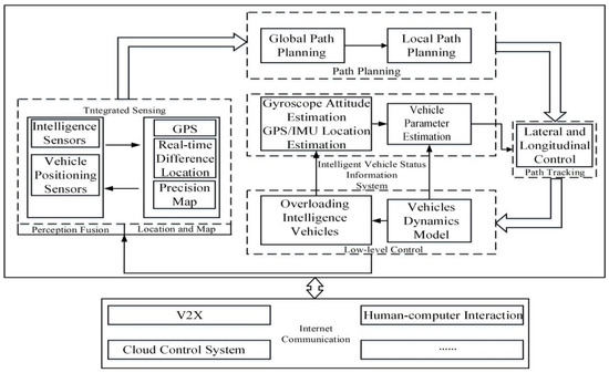
Figure 1.
Parameter estimation system of cargo intelligent vehicle.
2.1. Longitudinal Vehicle Dynamic Model
The load is shifted during longitudinal acceleration and deceleration of the vehicle. The CG position of the vehicle can be estimated by detecting the load change of the front and rear axles. As can be observed from Figure 2, a vehicle longitudinal dynamics model is established with the following assumptions made: The vehicle travels in a straight line without a lateral load while not considering lateral and roll motions. Air resistance, deformation of vehicle suspension and pitch angle change are ignored. The vehicle is symmetrical with the four wheels simplified into two front and rear axles.
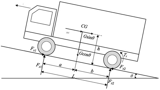
Figure 2.
Longitudinal vehicle dynamic model.
The vertical load of the front and rear axles of the vehicle can be expressed as:
where Fz1 and Fz2 are the front and rear axle vertical forces (N); L is the vehicle wheelbase (m); m is the vehicle mass (kg); a and b are the distances from CG of the vehicle to the front and rear axles (M); h is the height of CG (m); θ is the road gradient angle (rad); r is the wheel radius (m); and f is the rolling resistance coefficient. The vertical load Fz2 of the rear axle is measured by the load sensor.
2.2. State Space Model of CG Position
According to Equation (2), the vehicle speed v, the height of CG h and the distance a from CG to the front axle are regarded as the state variables. The height and the longitudinal position of CG can be considered as constants, and their derivatives with respect to time can be seen as zero. In that case, the differential equation can be expressed as:
The discretization of Equation (3) can be expressed as:
where Δt is the sampling period; vk and vk−1 represent the vehicle speed at t = k and t = k − 1, respectively; hk and hk−1 represent the heights of CG at t = k and t = k − 1, respectively; ak and ak−1 are the distance between CG at t = k and t = k − 1 from the front axle, respectively.
2.3. Overall Framework of Hybrid Estimation Algorithm
According to the vehicle dynamics model, a deep coupling effect can be observed between the longitudinal position and the vertical height of CG in the estimation process. Hence, an estimation algorithm combining HEKF and EKF was proposed by means of coefficient weighting. The flow chart of the algorithm is shown in Figure 3. The specific steps are as follows: firstly, set the initial state information and estimate the distance from the CG to the front axle at the current moment using the HEKF algorithm. Secondly, the height of CG is estimated twice, of which one was through HEKF, and the other was the estimation result of EKF together with the longitudinal position of CG. Moreover, weighting was performed on the height of CG obtained by the two algorithms to obtain the optimal estimation value of the height of CG at the current moment. Weighting is aimed at reducing the influence caused by the inaccurate estimation of the longitudinal position of CG at the previous moment. At last, the distance from CG to the front axle and the height of CG at the current moment are considered as the initial state at the next moment. The above steps are repeated. Two variables were decoupled from the nonlinear vehicle dynamics equation through repeated iteration.
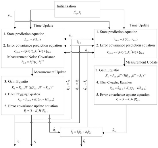
Figure 3.
Schematic of hybrid algorithm estimation.
The Kalman filter is the most widely used method for estimating the state of a vehicle. In comparison to other state estimation methods, the Kalman filter method is not only effective in correcting the error of the initial state, but it can also continuously adjust the predicted value of the system state based on the observations. Furthermore, the algorithm can filter system noise and reduce the negative impact of measurement noise, so we use Kalman filter to solve the problem of vehicle CG estimation.
2.4. Extended Kalman Filter Based on Huber
HEKF was rarely applied to vehicle parameter estimation in the study although it was proposed early in the related literature [28,29]. By Equation (4), the state equation can be obtained as:
where
The observation equation is presented below:
State and observation equations of the system constituted jointly by Equations (5) and (7) are:
where x and y stand for the state variable and the observation variable, respectively; f and H are the vector function and the measurement matrix of the process equation, respectively; W and V are the process noise and measurement noise, respectively.
The standard EKF filtering process is:
where
where Q and R are the covariance matrices of process noise and measurement noise, respectively; P is the error covariance; K is the Kalman gain.
Though EKF has been used in a great number of studies as a vehicle parameter estimation algorithm, it presents a frustrating flaw that the filtering performance will be severely degraded when the measurement noise exists an outlier observation with a high pollution rate rather than complying with the single Gaussian distribution [30]. Sensor measurement noise with a single Gaussian distribution is an ideal condition, because a large number of measurement outliers might exist due to electromagnetic interference, equipment aging, and data transmission errors in engineering applications. The Huber method is an estimation technique that combines the minimum l1 and l2 norms, which is robust to the situation of deviation from the assumed Gaussian distribution. Based on Huber’s generalized maximum likelihood method, a robust filtering technique can successfully address the issue of non-Gaussian noise distribution. EKF based on Huber’s estimation is a robust filter that can effectively improve the filter’s ability to restrain outliers, which is different from the standard EKF in terms of the filter gain:
where
where Ψz is the robustness factor.
The performances of HKF and KF are compared in a simulation environment, as shown in Figure 3. When the vehicle travels at a constant speed of approximately 15 m/s, the mixture probability density function of random measurement errors can be expressed by Equation (17) [31]:
where b is set to 5/. e is the perturbation coefficient, being 0.5. At this time, the measurement noise is a strong non-gaussian distribution. The vehicle speeds estimated using HKF and KF are shown in Figure 4a. Additionally, the errors between the two filtering algorithms and the true value are presented in Figure 4b.
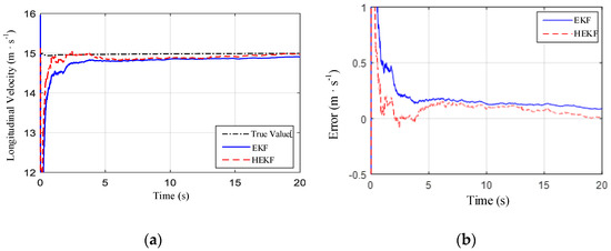
Figure 4.
Comparison of HKF and KF; (a) longitudinal speed and (b) error comparison.
As shown in Figure 4b, the red dotted line is always below than the blue solid line, indicating that the HKF method has a lower error than the KF method. It can be seen that HKF is superior to KF in terms of robustness and filtering accuracy when the measurement noise is interfered with by large outliers. The mean square error (MSE) is an important indicator to measure the error between the estimated value and the measured value. The results of the two algorithms under the working condition are shown in Table 1.

Table 1.
Comparison of HKF and KF.
2.5. Extended Kalman Filter
The EKF in this study estimated the height of CG making use of the longitudinal position of CG of the HEKF at the previous moment. Then, the heights of CG obtained by the two algorithms were weighted to obtain the optimal estimation value of the height of CG at the current moment. In that case, the vehicle speed v and the height of CG h are selected as state variables. With the longitudinal position information of CG a as an input, after discretization, it can be expressed as:
Through constructing the state and observation equations of the system, the flow of the EKF algorithm is shown in Equation (9) to Equation (13). The final result is obtained through continuous iteration.
3. Results
Joint simulations in MATLAB/Simulink and Trucksim are used to validate the effectiveness of the proposed estimation method. The vehicle dynamic is constructed in the heavy-duty vehicle simulation environment of TruckSim, and the vehicle’s CG estimation algorithm is executed in Matlab/Simulink. The vehicle is a van truck LCF Van 5.5 T/8.5 T (s_s) with air brake. The main parameters are shown in Table 2. In order to better prove the universality of the algorithm, two different driving modes of four-wheel drive (4 WD) and rear-wheel drive (RWD) are set. The road is divided into flat and variable gradient, and the simulation process is shown in Figure 5.
Table 2.
Basic parameters of the vehicle.
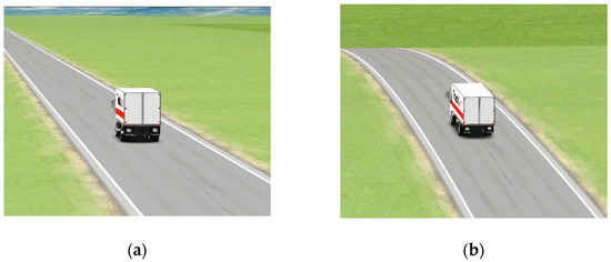
Figure 5.
Flat ground (a) and sloping ground (b) simulation.
3.1. Simulation Experiment
3.1.1. Four Wheel Drive Mode
(1) Flat ground
The initial speed of the vehicle is set to 15 km/h, the road adhesion coefficient is set to 0.85, and the sampling time interval is set to 0.02 s. The entire simulation time is 25 s. During this period, the vehicle performs longitudinal acceleration and deceleration. The state signal is shown in Figure 6a–d. The parameters and initial values of the HEKF-EKF algorithm are shown in Table 3.
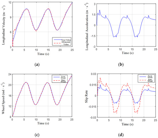
Figure 6.
Status signals of the 4 WD vehicle on the flat ground. (a) Longitudinal speed; (b) longitudinal acceleration; (c) wheel speed; (d) slip rate.
Table 3.
Parameters and initial values setting of the EKF/UKF estimator.
It can be seen from Figure 6a that the HEKF-EKF algorithm can filter out the noise signal well, the estimated value can be tracked accurately after 2 s, and the average absolute error between the estimated value and the real value in the whole process is 0.17 m/s. Figure 6b shows the change of the longitudinal acceleration of the vehicle. In order to ensure that the estimation algorithm can obtain an effective excitation signal, the maximum value is 2.1 m/s2 and the minimum value is −1.7 m/s2. In addition, as shown in Figure 5c,d, since it is a four-wheel drive vehicle, the rotational speed of the front and rear wheels is the same. Additionally, because the power output of the rear wheel of the cargo vehicle is larger than that of the front wheel, the slip rate of the rear wheel is slightly larger than that of the front wheel, but the overall remains within 3%, which meets the range requirements of the wheel slip rate in the literature [9].
The estimated result of CG of the four-wheel drive vehicle on a flat road is shown in Figure 7. The real value adopts the position of CG when the vehicle is static, that is, the distance between CG and the front axle is 1.5 m, and the height of CG is 1.03 m. It can be seen from the simulation results that the estimation of the distance between CG and the front axle of the two algorithms can reach the true value in about 2 s, but compared with the Huang model, the estimation result of the model in this paper is more stable, and the overall error is less than 2%. In addition, the Huang model estimates the height of CG at 1.2 m and tends to be stable in 10 s.
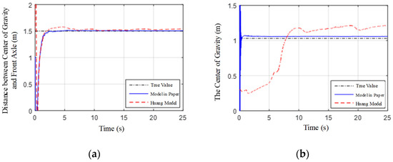
Figure 7.
Estimation results of the 4 WD vehicle on the flat ground. (a) Distance between CG and the front axle; (b) the center of gravity.
(2) Sloping ground
In order to verify the performance of the algorithm under the condition of sloped road, the slope as shown in Figure 8 is set. The maximum vertical height of the slope is 8 m, and the maximum slope angle is 6°.
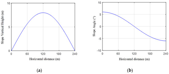
Figure 8.
Slope information. (a) Slope vertical height; (b) slope angle.
Similar to the simulation conditions of the flat road, the vehicle accelerates three times and decelerates two times during this period. Due to the increased slope and the large mass of the truck, the acceleration effect on the uphill process is not as obvious as that on the flat road. In the downhill section, the speed increases rapidly again, and its status signal is shown in Figure 9a–e.
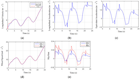
Figure 9.
Status signals of the 4 WD vehicle on the sloping ground. (a) Longitudinal speed; (b) longitudinal acceleration; (c) wheel speed; (d) equivalent acceleration; (e) slip rate.
The concept of equivalent acceleration β is defined in literature [9]. The larger the value of β, the better the estimation effect of the algorithm. The expression is as follows:
where θ is the road gradient angle (rad), ax is the vehicle longitudinal acceleration (m/s2), and Fa is the air resistance (N). Since the influence of ego vehicle acceleration, slope, and air resistance is considered, it is generally greater than the single longitudinal acceleration of the vehicle. This provides enough incentive for the realization of the estimation algorithm, and the equivalent acceleration of the whole process is shown in Figure 9c.
Figure 10 shows the estimation result of the position of CG of the four-wheel drive vehicle on a sloped road. It can be obtained that changing the road gradient increases the equivalent acceleration, and the maximum value is 2.6 m/s2. Under the action of a large excitation signal, compared with the model in this paper, the estimation result of the Huang model for the position of CG from the front axle can reach the true value faster, because the acceleration and wheel slip rate signals are 2.5 s, 8 s and 2.5 s, respectively. A mutation occurs at 16 s, so the estimation result also fluctuates at the corresponding position. Although the convergence speed of the model in this paper is 1 s slower, the estimated result curve is still stable. The results of the estimation of the height of CG are similar.
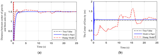
Figure 10.
Estimation results of the 4 WD vehicle on the sloping ground. (a) Distance between center of gravity and front axle; (b) the center of gravity.
3.1.2. Rear Wheel Drive Mode
(1) Flat ground
In this section, the current common rear-wheel drive mode of trucks is selected for verification. The change trend of speed and acceleration is the same as that of the previous working conditions, as shown in Figure 11a,b, and the wheel speed and slip rate are shown in Figure 6. Compared with four-wheel drive, the rotation speed of the rear wheel is significantly larger than that of the front wheel in the rear-wheel drive mode, and the rear wheel is the driving wheel, so the slip rate is positive, while the front wheel is the driven wheel, so the slip rate is negative. The maximum value is 0.06.
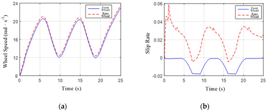
Figure 11.
Status signals of the RWD vehicle on the flat ground. (a) Wheel speed; (b) slip rate.
Figure 12 shows the estimation results of rear-wheel drive vehicles on flat roads. It can be seen that the estimated distance between CG of the Huang model and the front axle is 0.8 m, and the height of CG reaches 16 m, and the resultant divergence completely deviates from the true value. The reason is that the realization of the estimation algorithm needs to have enough longitudinal acceleration excitation (greater than 1.5 m/s2), under this condition, the rear wheel is used as the driving wheel, and the slip rate is greater than 0.03, which exceeds the limit of the slip rate that is required in literature [9]. It is worth noting that the model in this paper uses the signal of the vertical load state of the rear axle to avoid the influence of different driving modes of the car. Therefore, if the driving mode is changed, the algorithm can still quickly converge to near the true value. The results show that the average estimation errors of the longitudinal and vertical positions of CG of this model are both less than 2%.
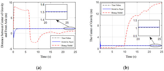
Figure 12.
Estimation results of the RWD vehicle on the flat ground. (a) Distance between the center of gravity and the front axle; (b) the center of gravity.
(2) Sloping ground
The road slope setting is the same as the previous working condition, as shown in Figure 8, and the state change of the entire simulation process is shown in Figure 13. Similar to flat road conditions, the rear wheels spin slightly faster than the front wheels and the wheel slip is positive. Since the vehicle is affected by the slope resistance, in order to achieve a similar speed effect, it needs to output stronger power, so the slip rate of the rear wheels will also be larger, the peak value will reach 0.08, and the slip rate of the front wheels will not change.
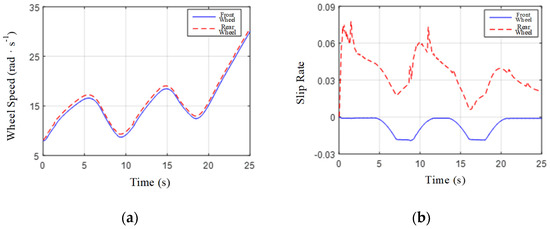
Figure 13.
Status signals of the RWD vehicle on the sloping ground. (a) Wheel speed; (b) slip rate.
Figure 14 shows the estimation results of the rear-wheel drive vehicle on a sloped road. It can be seen from the figure that the estimated distance between CG of the Huang model and the front axle is 1.2 m, and the height of CG reaches 12.6 m. The reason for the failure is that the wheel slip ratio exceeds the limit requirement.
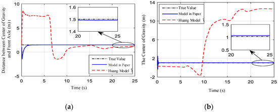
Figure 14.
Estimation results of the RWD vehicle on the sloping ground. (a) Distance between the center of gravity and the front axle; (b) the center of gravity.
3.2. Real Vehicle Experiment
This section provides real vehicle experimental validation of this estimation method, as shown in Figure 15. The truck is battery-powered, with four independent wheels. The truck used for experiments in this section was developed for Suzhou Automotive Research Institute and equipped with safety installations appropriate for automation and control experiments. All signals related to vehicle motion can be measured by the high-precision Oxford Technical Solution (OTS) RT3003 navigation system, which consists of an integrated dual-antenna differential GPS and inertial measurement unit. An active speed sensor is mounted on each wheel. A dSPACE MicroAutoBox controller was used on the vehicle, and the estimation algorithm was developed in Simulink. The vehicle state signals were obtained from the vehicle control unit (VCU) via chassis CAN. Data processing was done on a high-precision computer: Intel(R) Core (TM) i9-9900k CPU @ 3.60 GHz.
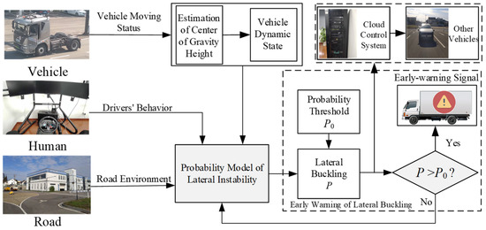
Figure 15.
Cloud control system and emergency warning of lateral buckling.
As a gesture to safety, this study adopts the remote driving mode. The driver operates Logitech G29 driving simulator to control the experimental truck. The longitudinal acceleration and deceleration of the vehicle are controlled by the gas and brake pedals, and the vehicle is kept in a straight line by the steering wheel. Then, the calculation of the probability of a lateral instability accident involving the truck is carried out based on the position of the center of gravity. This is the next step in our study and is not the research of this paper. The lateral instability probability of vehicle can be calculated on the cloud control system to reduce the calculation force and help vehicle to decide the most comfortable driving behavior on the premise of ensuring safety.
The proposed method for estimating CG position was evaluated under two road conditions. In the first test, the vehicle was driven on sloping ground. In the second test, the vehicle was kept on a flat ground. As shown in Figure 16 below.
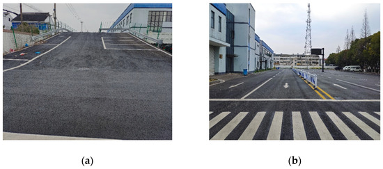
Figure 16.
Slope and flat ground information. (a) Sloping ground; (b) flat ground.
The road grade is critical for estimating the CG position. Altitude measurements available in a two-antenna GPS system for online road grade estimation were used in [32] and [33]. This paper takes a similar approach because the GPS systems are able to reach accuracy of up to 2 cm in the position measurement [9].
3.2.1. Four Wheel Drive Mode
(1) Flat ground
The estimated value of the height of CG of the vehicle is obtained by weighting the HEKF and EKF algorithms. Although there is jitter in the first 0.3 s, the overall convergence speed is faster, and the curve can be stabilized near the true value in only 1.5 s. At the same time, the estimated value is 1.06 m, with an error of 3%. When the vehicle is driving on a flat road, the algorithm’s estimation of the distance between CG and the front axle can reach the true value in about 2 s, as shown in Figure 17 below.
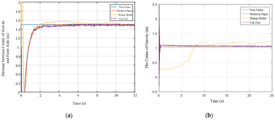
Figure 17.
Estimation results of the 4 WD vehicle on the flat ground. (a) Distance between the center of gravity and the front axle; (b) the center of gravity.
(2) Sloping ground
The results of the estimation of the height of CG are similar. Compared with the flat road, the estimated value of the Huang model has improved accuracy, but the curve fluctuates significantly, and the maximum deviation is 0.6 m. The test vehicle was driven on a sloped road, which was close to the simulated value. The estimation results of the model in this paper will not change with the sudden change of acceleration, and have stronger anti-interference ability, as shown in Figure 18 below.
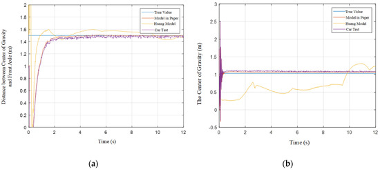
Figure 18.
Estimation results of the 4 WD vehicle on the flat ground. (a) Distance between the center of gravity and the front axle; (b) the center of gravity.
3.2.2. Rear Wheel Drive Mode
(1) Flat ground
When the vehicle is driving on a flat road, the algorithm can still quickly converge to near the true value. The results show that the average estimation errors of the longitudinal and vertical positions of CG of this model are both less than 2%, as shown in Figure 19 below.
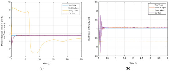
Figure 19.
Estimation results of the RWD vehicle on the flat ground. (a) Distance between the center of gravity and the front axle; (b) the center of gravity.
(2) Sloping ground
With the vehicle is driving on a sloping road, the estimated errors of the longitudinal position of CG and the vertical height of the test vehicle are both 2%, and they converge after 2 s and 1.5 s, respectively. Therefore, it is suitable for both four-wheel drive and rear-wheel drive models under different road conditions, as shown in Figure 20.
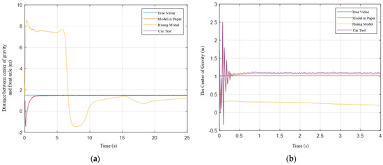
Figure 20.
Estimation results of the RWD vehicle on the sloping ground. (a) Distance between the center of gravity and the front axle; (b) the center of gravity.
3.3. Discussion
To sum up, according to the hybrid method of HEKF-EKF, the longitudinal and vertical positions of the vehicle’s center of gravity can be estimated effectively. The estimation error of the distance of CG to the front axle was less than 2%, and the estimated error of the height of CG was 3% with the convergence time of 2 s and 1.5 s, respectively. The proposed method outperforms existing estimation algorithms because it is applicable to a broader range of road conditions and driving methods with estimation, resulting in higher accuracy, stronger anti-interference performance, and a faster convergence rate, all of which contribute to road traffic safety.
In the intelligent network environment, GPS information is sent through the roadside equipment, and the vehicle GPS can obtain high precision dynamic position of the vehicle speed and heading angle information, the vehicle intelligent sensor to collect the driving state information of heavy vehicles, HEKF-EKF hybrid center of gravity position estimation method is used in the lateral instability warning problem of vehicles, lateral instability probability is calculated using the lateral instability probability model, and data is shared with other vehicles via the cloud control system.
4. Conclusions and Discussion
The method proposed in this paper outperforms the existing estimation algorithm and is applicable to a broader range of road conditions and driving modes. The algorithm has higher estimation accuracy, stronger anti-interference performance and faster convergence speed, which is conducive to road traffic safety. In the intelligent network environment, vehicle intelligent sensors collect the driving state information of heavy vehicles. Vehicle GPS can obtain vehicle speed and yaw angle information of high-precision dynamic position and send them through roadside equipment. The HEKF-EKF hybrid center of gravity position estimation method is used to solve the early warning problem of vehicle lateral instability. The lateral instability probability is calculated through the lateral instability probability model, and data is shared with other vehicles via the cloud control system.
Focusing on the 2-axle heavy duty vehicle with a rear axle load sensor, the CG position estimation algorithm was proposed through combining HEKF and EKF in the intelligent network environment on the basis of establishing the longitudinal dynamics model of the vehicle. The longitudinal position of CG and the vertical height can be accurately estimated through detecting the longitudinal speed and the vertical load signal of the rear axle.
Author Contributions
Conceptualization, F.W. and S.Z.; methodology, F.W. and C.S.; software, H.L.; investigation, F.W.; data curation, F.W. and C.S.; writing—original draft preparation, F.W.; writing—review and editing, C.S.; visualization, H.L.; funding acquisition, S.Z. All authors have read and agreed to the published version of the manuscript.
Funding
This work is supported by the National Natural Science Foundation of China (52002215); the Opening Fund of Key Laboratory of Transportation Industry of Automotive Transportation Safety Enhancement Technology (Chang’an University), PRC (300102221502); the Hubei Science and Technology Project (2021BEC005, 2021BLB225); the Suzhou Industrial Prospect and Key Technology Project (SYC2022078); the Natural Science Foundation of Jiangsu Province (BK20220243); and the Hong Kong Scholars Program (XJ2021028).
Data Availability Statement
Not applicable.
Conflicts of Interest
The authors declare no conflict of interest.
References
- Ma, Y.; Wang, Z.; Yang, H.; Yang, L. Artificial intelligence applications in the development of autonomous vehicles: A survey. IEEE/CAA J. Autom. Sin. 2020, 7, 315–329. [Google Scholar] [CrossRef]
- Shen, B.; Zhang, Z.; Liu, H.; Li, S.; Zhao, L. Research on a Conflict Early Warning System Based on the Active Safety Concept. J. Adv. Transp. 2018, 2018, 8372108. [Google Scholar] [CrossRef]
- Sun, C.; Zheng, S.; Ma, Y.; Chu, D.; Yang, J.; Zhou, Y.; Li, Y.; Xu, T. An active safety control method of collision avoidance for intelligent connected vehicle based on driving risk perception. J. Intell. Manuf. 2021, 32, 1249–1269. [Google Scholar] [CrossRef]
- Rodríguez, A.J.; Sanjurjo, E.; Pastorino, R.; Naya, M.Á. State, parameter and input observers based on multibody models and Kalman filters for vehicle dynamics. Mech. Syst. Signal Process. 2021, 155, 107544. [Google Scholar] [CrossRef]
- Xing, Y.; Lv, C. Dynamic State Estimation for the Advanced Brake System of Electric Vehicles by Using Deep Recurrent Neural Networks. IEEE Trans. Ind. Electron. 2020, 67, 9536–9547. [Google Scholar] [CrossRef]
- Jin, Z.; Zhang, L.; Zhang, J.; Khajepour, A. Stability and optimised H∞ control of tripped and untripped vehicle rollover. Veh. Syst. Dyn. 2016, 54, 1405–1427. [Google Scholar] [CrossRef]
- He, Y.; Yan, X.; Lu, X.-Y.; Chu, D.; Wu, C. Rollover risk assessment and automated control for heavy duty vehicles based on vehicle-to-infrastructure information. IET Intell. Transp. Syst. 2019, 13, 1001–1010. [Google Scholar] [CrossRef]
- Park, G.; Choi, S.B. An Integrated Observer for Real-Time Estimation of Vehicle Center of Gravity Height. IEEE Trans. Intell. Transp. Syst. 2021, 22, 5660–5671. [Google Scholar] [CrossRef]
- Huang, X.; Wang, J. Real-Time Estimation of Center of Gravity Position for Lightweight Vehicles Using Combined AKF–EKF Method. IEEE Trans. Veh. Technol. 2014, 63, 4221–4231. [Google Scholar] [CrossRef]
- Qu, S.; Wang, W.; Wan, J.; Gu, Z.; Yang, J.; Chu, D. Curve Speed Modeling and Factor Analysis Considering Vehicle-road Coupling Effect. In Proceedings of the 2019 5th International Conference on Transportation Information and Safety (ICTIS), Liverpool, UK, 14–17 July 2019; pp. 1127–1131. [Google Scholar]
- Lee, J.; Hyun, D.; Han, K.; Choi, S. Real-Time Longitudinal Location Estimation of Vehicle Center of Gravity. Int. J. Automot. Technol. 2018, 19, 651–658. [Google Scholar] [CrossRef]
- Bascetta, L.; Ferretti, G. LFT-Based Identification of Lateral Vehicle Dynamics. IEEE Trans. Veh. Technol. 2022, 71, 1349–1362. [Google Scholar] [CrossRef]
- Lin, C.; Gong, X.; Xiong, R.; Cheng, X. A novel H∞ and EKF joint estimation method for determining the center of gravity position of electric vehicles. Appl. Energy 2017, 194, 609–616. [Google Scholar] [CrossRef]
- Attia, T.; Vamvoudakis, K.G.; Kochersberger, K.; Bird, J.; Furukawa, T. Simultaneous dynamic system estimation and optimal control of vehicle active suspension. Veh. Syst. Dyn. 2019, 57, 1467–1493. [Google Scholar] [CrossRef]
- Wenzel, T.A.; Burnham, K.J.; Blundell, M.V.; Williams, R.A. Dual extended Kalman filter for vehicle state and parameter estimation. Veh. Syst. Dyn. 2006, 44, 153–171. [Google Scholar] [CrossRef]
- Rozyn, M.; Zhang, N. A method for estimation of vehicle inertial parameters. Veh. Syst. Dyn. 2010, 48, 547–565. [Google Scholar] [CrossRef]
- Cheng, C.; Cebon, D. Parameter and state estimation for articulated heavy vehicles. Veh. Syst. Dyn. 2011, 49, 399–418. [Google Scholar] [CrossRef]
- Yue, H.; Zhang, L.; Shan, H.; Liu, H.; Liu, Y. Estimation of the vehicle’s centre of gravity based on a braking model. Veh. Syst. Dyn. 2015, 53, 1520–1533. [Google Scholar] [CrossRef]
- Zheng, H.; Ma, S.; Liu, Y. Vehicle braking force distribution with electronic pneumatic braking and hierarchical structure for commercial vehicle. Proc. Inst. Mech. Eng. Part I J. Syst. Control Eng. 2018, 232, 481–493. [Google Scholar] [CrossRef]
- Fu, Z.; Hu, Q.; Li, B. Adaptive online estimation of centre of gravity height for commercial vehicles. Int. J. Heavy Veh. Syst. 2021, 28, 206–225. [Google Scholar] [CrossRef]
- Solmaz, S.; Akar, M.; Shorten, R.; Kalkkuhl, J. Real-time multiple-model estimation of centre of gravity position in automotive vehicles. Veh. Syst. Dyn. 2008, 46, 763–788. [Google Scholar] [CrossRef]
- Reineh, M.S.; Enqvist, M.; Gustafsson, F. IMU-based vehicle load estimation under normal driving conditions. In Proceedings of the 53rd IEEE Conference on Decision and Control, Los Angeles, CA, USA, 15–17 December 2014; pp. 3376–3381. [Google Scholar]
- Imine, H.; Fridman, L.; Madani, T. Identification of vehicle parameters and estimation of vertical forces. Int. J. Syst. Sci. 2015, 46, 2996–3009. [Google Scholar] [CrossRef]
- Yu, Z.; Wang, J. Simultaneous Estimation of Vehicle’s Center of Gravity and Inertial Parameters Based on Ackermann’s Steering Geometry. J. Dyn. Syst. Meas. Control 2017, 139, 031006. [Google Scholar] [CrossRef]
- Deng, Z.; Chu, D.; Tian, F.; He, Y.; Wu, C.; Hu, Z.; Pei, X. Online estimation for vehicle center of gravity height based on unscented Kalman filter. In Proceedings of the 2017 4th International Conference on Transportation Information and Safety (ICTIS), Banff, AB, Canada, 8–10 August 2017; pp. 33–36. [Google Scholar]
- Rajamani, R.; Piyabongkarn, D.; Tsourapas, V.; Lew, J.Y. Parameter and State Estimation in Vehicle Roll Dynamics. IEEE Trans. Intell. Transp. Syst. 2011, 12, 1558–1567. [Google Scholar] [CrossRef]
- González, D.; Pérez, J.; Milanés, V.; Nashashibi, F. A Review of Motion Planning Techniques for Automated Vehicles. IEEE Trans. Intell. Transp. Syst. 2016, 17, 1135–1145. [Google Scholar] [CrossRef]
- Boncelet, C.G.; Dickinson, B.W. An approach to robust Kalman filtering. In Proceedings of the 22nd IEEE Conference on Decision and Control, San Antonio, TX, USA, 14–16 December 1983; pp. 304–305. [Google Scholar]
- Karlgaard, C.D.; Schaub, H. Huber-Based Divided Difference Filtering. J. Guid. Control Dyn. 2007, 30, 885–891. [Google Scholar] [CrossRef]
- Agamennoni, G.; Nieto, J.I.; Nebot, E.M. An outlier-robust Kalman filter. In Proceedings of the 2011 IEEE International Conference on Robotics and Automation, Shanghai, China, 9–13 May 2011; pp. 1551–1558. [Google Scholar]
- Karlgaard, C.; Schaub, H. Adaptive huber-based filtering using projection statistics: Application to spacecraft attitude estimation. In Proceedings of the AIAA Guidance, Navigation and Control Conference and Exhibit, Honolulu, HI, USA, 18–21 August 2008; p. 7389. [Google Scholar]
- Bae, H.; Ryu, J.; Gerdes, J. Road Grade and Vehicle Parameter Estimation for Longitudinal Control Using GPS. In Proceedings of the IEEE Conference on Intelligent Transportation Systems, Oakland, CA, USA, 25–29 August 2001; pp. 166–171. [Google Scholar]
- Sahlholm, P.; Johansson, K.H. Road grade estimation for look-ahead vehicle control using multiple measurement runs. Control Eng. Pract. 2010, 18, 1328–1341. [Google Scholar] [CrossRef]


Disclaimer/Publisher’s Note: The statements, opinions and data contained in all publications are solely those of the individual author(s) and contributor(s) and not of MDPI and/or the editor(s). MDPI and/or the editor(s) disclaim responsibility for any injury to people or property resulting from any ideas, methods, instructions or products referred to in the content. |
© 2023 by the authors. Licensee MDPI, Basel, Switzerland. This article is an open access article distributed under the terms and conditions of the Creative Commons Attribution (CC BY) license (https://creativecommons.org/licenses/by/4.0/).