Article

A Potent Fractional-Order Controller for Interconnected Multi-Source Microgrids

by
Ioannis Moschos
*,
Ioannis Mastoras
and
Constantinos Parisses
Department of Electrical and Computer Engineering, University of Western Macedonia, ZEP Campus, 50100 Kozani, Greece
*
Author to whom correspondence should be addressed.
Electronics 2023, 12(19), 4152; https://doi.org/10.3390/electronics12194152
Submission received: 16 July 2023 / Revised: 16 September 2023 / Accepted: 4 October 2023 / Published: 6 October 2023

Abstract

:
Frequency deviations and the capability to cope with demand are two of the main problems in isolated or interconnected microgrids, especially with the increase in the penetration level of renewable energy sources. Those two problems call for new improved controllers and methods able to suppress frequency deviations while keeping a balance between supply and demand. This study focuses on the implementation of a filtered fractional-order PDF controller in series with a one plus fractional-order PI controller (FOPDF-(1+FOPI)) for the frequency regulation of three-area multi-source interconnected microgrids. The proposed controller is optimized via the coot optimization algorithm. The proposed microgrids incorporate various sustainable units, renewable energy sources and a hybrid energy storage system in each area. The microgrids consist solely of sustainable and renewable sources and aim to provide possible microgrid configurations for 100% sustainable microgrids, which could be farms or small communities. The proposed controller is compared with the PIDF, integer-order PDF-(1+PI), and FOTDF-(1+TI) controllers in various scenarios. The first scenario involved evaluating the proposed controller in an isolated microgrid, where it achieved the best ITAE value, outperforming the second best by 29.5%. The second scenario considered three-area interconnected microgrids without RES penetration. The results revealed that the FOPDF-(1+FOPI) controller reduced the settling time in area one by 79.13% and 52.26% compared to that of the PIDF and FOTDF-(1+TI) controllers. Next, RES penetration was introduced into each microgrid in the form of steps or varied changes. Subsequently, performance evaluation was conducted in the presence of a communication time delay and noise in the control channels. Finally, a robustness assessment was conducted for the proposed controller in the interconnected microgrids with respect to parameter uncertainties. The simulations showed a maximum deviation in the settling time and maximum overshoot in area 1 of 66.6% and 38.74%, respectively

1. Introduction

As global power consumption continues to rise while conventional fossil fuel resources dwindle, there is a growing need to transition to renewable energy sources (RESs) in order to meet increasing demand and reduce CO2 emissions [1]. Among the established and widely recognized RESs, solar and wind resources in the form of photovoltaic (PV) and wind turbine generation have emerged as prominent solutions [2,3], followed by sea wave energy, which is abundant in oceans and has not been fully utilized. However, the intermittent characteristics of solar, wind, and ocean energy sources prevent them from providing a consistent and reliable energy supply to meet the demand. This volatility also poses challenges in maintaining the balance between energy generation and consumption. Furthermore, they degrade the overall reliability and stability of the connected power systems [4]. A frequently utilized method to improve stability and flexibility involves incorporating energy storage systems (ESSs).
Another possible approach that can work in parallel with RESs is the use of bioenergy obtained from hazardous environmental waste generated by current living habits. This strategy entails the transformation of waste materials into bioenergy and blending it with RESs and ESSs to satisfy demand. By putting this approach into practice, waste generation is decreased while simultaneously fostering a long-term strategy for reaching net-zero emissions of greenhouse gases. Although bioenergy cannot fulfill the global demand alone, it can be used with RESs and ESSs to construct sustainable microgrids in remote farms or towns. This integration will allow remote communities and farms to meet their energy demand while at the same time alleviating hazardous waste [5].
Organic and agricultural biodegradable trash may be gathered and converted into fuel for biogas and biodiesel production units. The anaerobic digestion of biodegradable substances such as animal waste, agricultural waste, food waste, and sewage produces biogas, which consists of methane (CH4), carbon dioxide (CO2), and hydrogen sulfide (H2S) [6]. The biogas produced can be used as fuel in a biogas turbine generator (BGTG) to generate electrical power [7]. Biodiesel is a sustainable fuel made from vegetable oils and animal fats using a process known as transesterification. Biodiesel is a biodegradable fuel that does not include toxic ingredients such as sulfur or benzene [8]. The biodiesel produced can be utilized as a fuel for a biodiesel turbine generator (BDEG) to produce electricity [9,10]. In addition, wastewater and rainwater could be collected and used to power a micro-hydro turbine generator (MHTG) after it is cleaned and filtered [11]. Finally, a biomass combined heat and power unit (BCHP) could generate electricity using agricultural wastes and appropriately processed non-recycled waste materials [12].
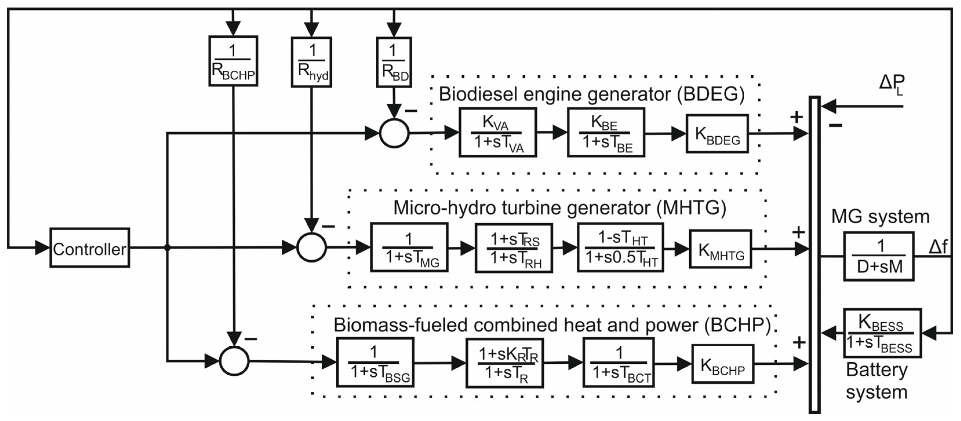
The major issues faced by interconnected or isolated microgrids that consist of bioenergy or conventional units and are relevant to current power systems center around reducing voltage and frequency deviations from the system’s nominal values. These variations occur because of the unpredictable nature of RESs and changes in consumer demand profiles brought on by contemporary living. Any deviations from the nominal values may cause equipment damage or compromise the quality of the electricity produced. Voltage deviations can arise due to changes in the load power factor. Automatic voltage regulators (AVRs) are used to avoid such behavior and keep the terminal voltage within operational limits. AVRs are used in power plants, especially on synchronous generators, with the primary goal of keeping the voltage at its nominal value [13,14]. Load frequency control (LFC) is used in the power generation industry to address and mitigate frequency aberrations while maintaining a supply and demand balance. LFC is a mechanism that regulates the power output to ensure that the frequency of the electrical system does not deviate from the acceptable limits. This is performed by monitoring the frequency and adjusting power generation accordingly. By implementing ESSs or hybrid energy storage systems (H-ESSs) and designing better controllers, it is possible to further mitigate frequency and voltage aberrations.
Over the last few decades, academics have investigated various control solutions to handle LFC in power systems of differing scales and technologies, isolated or interconnected. In [15], a two-area system with a HVDC link and a time delay was taken into consideration. The LFC of the linked system was carried out using a distributed-order proportional–integral–derivative (DOPID) controller. In [16], a model predictive controller was used for the LFC of a two-area interconnected system consisting of a PV and thermal unit. Reference [17] introduced a fuzzy PID controller with a fractional integrator and filter (PIλDF) for the LFC of a three-area system. The authors in [18] conducted a stability analysis of a LFC system, consisting of a thermal unit, demand response control and an electric vehicle aggregator. To conduct a delay-dependent stability analysis of the LFC and determine the stability zone, an improved Lyapunov–Krasovskii functional (LKF) was employed. The LKF incorporated time-varying delays by utilizing linear matrix inequalities. A two-area interconnected power system was studied in [19]. The authors utilized a PI/PD dual-mode controller for frequency regulation.
The current studies on LFC in isolated or interconnected microgrids encompass an array of methodologies and techniques. A PID controller tuned via the particle swarm optimization–gravitational search algorithm (PSO-GSA) was implemented for an islanded microgrid in [20]. The study included the following generating units: a PV unit, diesel generator, and wind turbine generator. In addition, the proposed microgrid incorporated a fuel cell, an aqua electrolyzer, a battery energy storage system, and a flywheel energy storage system. However, the proposed system did not consider any bioenergy units and the PID controller was implemented in an isolated microgrid. The authors in [9] utilized a filtered fractional-order proportional–derivative (FOPDF) controller in series with a one plus fractional-order proportional–integral (1+FOPI) controller for an isolated microgrid consisting of diverse bioenergy units, RESs, a battery energy storage system, an aqua electrolyzer, and a fuel cell. Yet, a H-ESS was not considered and the proposed controller was applied to an isolated microgrid. In [21], a combined fractional and integer-order master–slave controller was suggested for the LFC of two-area interconnected microgrids. The first microgrid consisted of a diesel engine generator, a wind turbine generator, an aqua electrolyzer, and a fuel cell. The second microgrid consisted of a PV unit and a diesel engine generator. In addition, electric vehicles have been considered in both microgrids. However, the study did not include a H-ESS or a multisource configuration for microgrids. A PID controller for an isolated renewable microgrid was proposed in reference [1]. The study included only a battery energy storage system, and the frequency deviation was studied for an isolated microgrid. Reference [22] employed a robust observer sliding mode controller for three-area interconnected microgrids. Each area comprised a non-reheat power plant, and the first and second included a wind turbine generator. However, a multi-source interconnected system with a H-ESS was not considered. In reference [23], a proportional–integral (PI) controller was implemented in an isolated microgrid. The microgrid consisted of various sources, yet it did not incorporate any bioenergy units. In reference [24], a fuzzy PID controller was applied to a microgrid with an energy storage system and a reheat thermal power plant. However, the controller was applied to an isolated microgrid without incorporating any bioenergy units.
A fractional-order proportional–integral–derivative (FOPID) controller, tuned via cohort intelligence optimization, was proposed in [25] for the frequency regulation of a single-area microgrid and two-area interconnected microgrids. The microgrids consisted of a distributed energy system and a thermal unit. The authors in [26] proposed the symbiotic organism search algorithm for the tuning of a FOPID controller in two-area interconnected microgrids. The proposed system included a hybrid energy storage unit, renewable energy sources and two conventional units. Reference [27] proposed a fuzzy FOPID controller for a single-area microgrid consisting of a H-ESS, RES, and a diesel generation unit. However, the performance of the fractional-order controllers in multi-source or multi-area microgrids was not tested in any of the three aforementioned studies. In [28], a fractional-order PI controller cascaded with a fractional-order tilt-derivative (TDμ) controller was implemented for a single-area microgrid, comprising a thermal unit, wind power plant, and photovoltaic power plant. In addition, an ESS was considered in the system, while the cascaded controller parameters were optimized using the kidney-inspired algorithm. However, the proposed system considered only one conventional unit without including any bioenergy units, multi-sourced microgrids, or a H-ESS. An adaptive fuzzy FOPD–FOPI controller was implemented in [29] for a standalone microgrid. Although the study considered RESs, a H-ESS, and a diesel engine generator, it did not incorporate any bioenergy units or diverse generation units.
From the presented studies, it is evident that the majority incorporate an integer PID or PI controller in isolated microgrids with RESs. A small number of them implement a H-ESS or bioenergy units. The studies of interconnected microgrids consist of two- or three-area systems, without considering multi-source generation. A small fraction of them incorporate bioenergy units and fractional-order controllers.
However, just as power systems evolve, similar evolution must occur in the controllers employed within these systems. This implies the need to develop new controllers and tuning methods aimed at enhancing the performance and robustness of the controlled systems. In view of the aforementioned, a new controller is proposed, tuned via the newly introduced coot optimization algorithm, for the frequency regulation of a three-area interconnected multi-sourced system containing only sustainable units, RESs and a different H-ESS in each area. The current study is an extended version of the conference paper that was presented in HAICTA 2022 [9].
The proposed study brings forth the following notable contributions:
  • A proficient scheme of three multi-source interconnected microgrids.
  • The incorporation of bioenergy units, RESs, and H-ESSs.
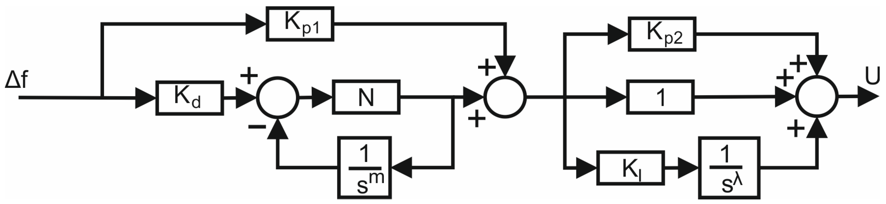
  • A comparison of the proposed FOPDF-(1+FOPI) controller with the integer-order PDF-(1+PI), FOTDF-(1+TI), and PIDF controllers.
  • The utilization of the coot optimization algorithm (COA) for tuning the controllers’ parameters.
  • An evaluation of the controllers’ performance for the simultaneous penetration of RESs in all areas.
  • The ability of the controllers to effectively attenuate noise injected into the area control error channels of the system.
The remainder of the paper is structured as follows: Section 2 outlines and analyzes the microgrids under study; Section 3 presents the controllers considered; next, the COA is described; subsequently, the results are presented and discussed, followed by the conclusion of the paper.

2. Power Systems

2.1. Microgrids under Study

Isolated microgrids, in order to cope with the demand, need to comprise various energy sources and ESSs to guarantee that the balance between demand and generations is kept. The current study considers two systems: (i) an isolated microgrid with ESS and bioenergy units as depicted in Figure 1 and (ii) a three-area interconnected microgrid consisting of H-ESSs, RESs, and bioenergy units as depicted in Figure 2. The isolated microgrid comprises three generating units: (i) a biodiesel engine generator, (ii) a micro-hydro turbine generator, and (iii) a biomass-fueled combined heat and power unit. Each of these units is associated with its respective participation factor, denoted as KBDEG, KMHTG, KBCHP, and the droop constant. Furthermore, the isolated microgrid includes a BESS. In the three-area interconnected microgrid, the first microgrid consists of five generating units: (i) a geothermal power plant, (ii) a biodiesel engine generator, (iii) a micro-hydro turbine generator, (iv) a biogas turbine generator, and (v) a biomass-fueled heat and power unit. Each of these units is associated with its respective participation factor, denoted as KGTPP, KBDEG, KMHTG, KBGTG, KBCHP, and droop constant R1, as well as the tie-lines interconnecting it with the second (ΔP12) and third (ΔP13) microgrid. Additionally, the microgrid includes an ORC solar thermal power plant, sea wave energy, and a H-ESS, which consists of a BESS and superconducting energy storage system (SMES). The second interconnected microgrid consists of five generating units: (i) a wind power plant, (ii) a biodiesel engine generator, (iii) a micro-hydro turbine generator, (iv) a biogas turbine generator, and (v) a biomass-fueled heat and power unit. Each of these units is associated with its respective participation factor, denoted as KWPP, KBDEG, KMHTG, KBGTG, KBCHP, and droop constant R2, and the tie-line interconnecting it with the third (ΔP23) microgrid. Furthermore, the microgrid includes an ORC solar thermal power plant and a H-ESS, which comprises a BESS and flywheel energy storage system (FESS). The third interconnected microgrid consists of five generating units: (i) a biomass-fueled heat and power unit, (ii) a biogas turbine generator, (iii) a geothermal power plant, (iv) a biodiesel engine generator, and (v) a wind power plant. Each of these units is associated with its respective participation factor, denoted as KBCHP, KBGTG, KGTPP, KBDEG, KWPP, and droop constant R3. Moreover, the microgrid includes a PV unit and H-ESS, which comprises a BESS and supercapacitor energy storage system (SCES).
The transfer functions of the generation units, ESSs, and RESs are presented in the following subsection. The parameters of the microgrids used in the simulations are gathered in Table 1.

2.2. Mathematical Modeling of the Proposed Microgrids

2.2.1. Generating Units and RESs

The transfer function for the BDEG includes the inlet valve and turbine (Equation (1)). The BGTG consists of the inlet -valve, governor, combustor, and turbine, with its transfer function being presented in Equation (2). The BCHP includes the speed governor, re-heater, and turbine. The transfer function for the BCHP is described via Equation (3). Equation (4) represents the transfer function of the MHTG, which encompasses the speed governor, penstock, and micro-hydro turbine. The GTPP consists of the governor and turbine, described by Equation (5), while the WPP comprises of the pitch actuator and blade characteristics as expressed in Equation (6).
G B D E G s = 1 s T V A + 1 1 s T B E + 1
G B G T G s = 1 + X c s 1 + Y c s 1 + b B s 1 + T C R s 1 + T B G s 1 1 + T B T
G B C H P s = 1 1 + T B S G s 1 + K R T R s 1 + T R s 1 1 + T B C H P
G M H T G s = 1 1 + T M G s 1 + T R S s 1 + T R H s 1 T H T s 1 + 0.5 T H T s
G G T P P s = 1 1 + T G G s 1 1 + T G T s
G W P P s = K P 2 1 + T P 2 s K P 3 K P C 1 + s T P 1 1 + s 1 + s
To optimize and test the design of the proposed power systems, and effectively utilize the RESs introduced in the proposed systems, various RESs such as PV, organic Rankine cycle solar thermal power plant (ORC-STPP) and sea wave energy (SWE) are considered. PV panels could be installed on the roofs of residential buildings, livestock barns, and storage buildings that contain organic foods, such as wheat. A linear Fresnel reflector (LFR) type combined with a thermal oil-based organic Rankine cycle (ORC) is being considered for the solar thermal power plant (STPP) because it requires a smaller land area compared to the parabolic trough collector (PTC), making it a better choice for remote communities or farms with limited available land. The transfer functions of the PV panel and ORC-STPP are expressed as follows:
G P V s = K P V 1 + T P V s
G S T P P s = K L F R 1 + T L F R s K O R C T H X 1 + T H X s 1 1 + T S T s
Finally, the proposed microgrids could harness the energy stored in the ocean. This technology utilizes the temperature difference between the ocean’s surface and depth to power a low-pressure turbine. The conversion of wave energy into electrical power is achieved through wave energy converters. The mathematical model of SWE includes the wave governor and turbine, as follows [30]:
G S W E s = 1 1 + T S W G s 1 + T S W T s

2.2.2. Energy Storage Systems

In the isolated microgrid, only a battery energy storage system (BESS) is considered. In the interconnected microgrids, three different combinations of H-ESSs are considered in each microgrid, comprising BESS/SMES, BESS/FESS, and BESS/SCES. The mathematical formulas of each storage system are expressed in Equations (10)–(13).
G B E S S s = K B E S S 1 + T B E S S s ,
G S M E S s = K S M E S 1 + T S M E S s ,
G F E S S s = K F E S S 1 + T F E S S s ,
G S C E S s = K S C E S 1 + T S C E S s

2.2.3. Load Generator Model

Equation (14) [13] uses 50% loading for a low inertia system at a nominal frequency of 50 Hz to describe the dynamics of the generator load for the jth microgrid.
Δ f j = 1 D j + 2 H j s Δ P j

3. Controller Structure

Fractional calculus is a mathematical framework that generalizes classical integration and differentiation into real numbers. In the field of control engineering, there has been growing interest in the application of fractional-order (FO) controllers. This interest stems from the superior performance exhibited by FO controllers when compared to that of integer-order (IO) controllers.
In the current research, a filtered fractional-order proportional–derivative controller in series with a one plus fractional-order proportional–integral controller is proposed for the LFC of the suggested isolated and interconnected microgrids. The parameters of the controller are tuned via the coot optimization algorithm. The transfer function of the controller is expressed in Equation (15) and the schematic in Figure 3.
G F O P D F 1 + F O P I s = K p 1 + K d N s m N + s m 1 + K p 2 + K I s λ
In addition, the newly proposed controller is compared with the filtered proportional integral derivative controller (PIDF), the filtered IO PDF-(1+PI) controller, and the filtered fractional-order tilt-derivative (FOTDF) in series with a tilt-integral controller (TI). The block diagram of the first two controllers is depicted in Figure 4 and their transfer functions are defined in Equations (16) and (17), respectively. The block diagram of the FOTDF-(1+TI) controller is shown in Figure 5 and its transfer function is defined in Equation (18). For the calculation of the fractional terms, the refined Oustaloup filter was used through the FOMCON toolbox [31]. For a comprehensive analysis of the definitions and approximations in fractional calculus, interested readers can refer to [32].
G P I D F s = K p + K I s + K d s N s + N
G P D F 1 + P I s = K p 1 + K d N s N + s 1 + K p 2 + K I s
G F O T D F 1 + T I = K t 1 s 1 n 1 + K d N s m N + s m 1 + K t 2 s 1 n 2 + K I s

4. Coot Optimization Algorithm

Based on the observation of coots swimming together, researchers Iraj Naruei and Farshid Keynia [33] developed a swarm-based metaheuristic optimization algorithm called coot optimization algorithm. The algorithm takes advantage of the collective behavior of coots and applies it to solve complex optimization problems.
Coots move in a chain formation, led by a group of leaders, to their chosen location, which is generally a food supply. The COA is modeled after this behavior and includes four separate movements that coots make on the water’s surface: (i) random movement, (ii) chain movement, (iii) position modification dependent on the leaders, and (iv) leaders directing the group to the best location. The search area is first filled with a random population by the COA. The population is then subjected to repeated evaluations of the objective function up until the maximum number of iterations is attained. The ITAE criterion is used as the objective function to be minimized, as follows:
I T A E = 0 t s i m t j n Δ f j + Δ P t i e , j d t
The initial population is generated by using the following expression:
C o o t P o s i = r a n d 1 , d . u b l b + l b
where CootPos stands for the coot position, I stands for the coot’s index number, d stands for search space dimension, and ub and lb stand for the search space’s upper and lower limits. The fitness of each coot is assessed once the initial population is produced by estimating the objective function. The COA then executes the four distinct moves. Equation (21) describes the first movement, which consists of the coot traveling toward a place that is randomly selected within the search space.
Q = r a n d 1 , d . u b l b + l b
The introduction of the random movement is essential in preventing the algorithm from becoming trapped in local optima. When the algorithm falls within a local optimum area, the random movement enables the agents (coots) to leave this region and explore other regions within the search space. This way, the probability of finding better solutions is increased. The calculation of the new position is derived from Equation (22):
C o o t P o s i = C o o t P o s i + A R 2 Q C o o t P o s i
where A = 1-iter/Max_iter and R2 is an arbitrary value between 0 and 1. The COA determines the average location of two coots using the following formula in order to carry out chain movement:
C o o t P o s i = 0.5 C o o t P o s i 1 + C o o t P o s i ,
where CootPos(i—−1) stands in for the second coot. The third COA movement involves modifying the position in accordance with the group leaders. A leader is picked in this movement using Equation (24), where i is the index number of the present coot, NL is the number of leaders, and K is the index number of the leader:
K = 1 + i m o d N L
The coot moves toward the leader’s location by applying the following expression to the leader with the index number, K:
C o o t P o s i = L e a d e r P o s K + 2 R 1 cos 2 R π L e a d e r P o s K C o o t P o s i ,
where CootPos is the current position of the coot, LeaderPos(K) is the position of the chosen leader, R1 is a random number between 0 and 1, and R is an arbitrary number between −1 and 1. Equation (25) modifies the coot’s position to be closer to the leader’s position, introducing some randomness to promote exploration within the search space. In the last movement of the algorithm, the group leaders update their position toward the optimal area by using the following formula:
L e a d e r P o s i = B R 3 cos 2 R π g B e s t L e a d e r P o s i + g B e s t ,   R 4 < 0.5 B R 3 cos 2 R π g B e s t L e a d e r P o s i g B e s t ,   R 4 0.5
where B is determined by B = 2-iter/Max_iter, gBest is the best location ever found, R3 and R4 are arbitrary numbers between 0 and 1, R is an arbitrary number between −1 and 1, and R is a random number between −1 and 1.
Formula (26) is used to investigate and look for better positions close to the leader’s present position. The introduction of the term BR3 enables the algorithm to concurrently explore and exploit the search space by allowing greater random movements to be carried out. Additionally, the term cos(2πR) is used to examine the area surrounding the best coot location with varied radiuses in an effort to find possible superior positions nearby.
To maintain the random nature of the algorithm, movements are chosen randomly. Figure 6 illustrates the COA methodology, offering a comprehensive overview of the different steps it encompasses. In this proposed approach, the controller’s parameters represent the positions of coots, and their desired destination, expressed via the objective function in Equation (19), corresponds to a food source. The algorithm commences by randomly generating a population of coots and computing the objective function’s value for each coot. Subsequently, the process outlined in Figure 6 is executed repeatedly until the maximum number of iterations is attained.

5. Results

In this section, the performance of the proposed single-area and three-area interconnected microgrids is assessed, as discussed in Section 2, as well as that of the filtered FOPDF controller in series with a 1+FOPI controller in regulating the frequency of the microgrids. The simulations utilize the COA to determine the optimal values of the controllers. Initially, the COA is compared to a state-of-the-art optimization method from the existing literature. Next, the scenarios that follow are taken into consideration in order to evaluate the performance, disturbance rejection, and robustness of the proposed controller and compare it to the other three controllers discussed in Section 3.
  • Scenario 1: Isolated microgrid with ESS and bioenergy units.
  • Scenario 2: Three-area interconnected microgrids with bioenergy, H-ESSs, and the absence of RES penetration.
  • Scenario 3: Three-area interconnected microgrids with bioenergy, H-ESSs, ORC-STTP penetration, and PV penetration.
  • Scenario 4: Three-area interconnected microgrids with bioenergy, H-ESSs, ORC-STTP penetration, PV penetration, and SWE penetration.
  • Scenario 5: Three-area interconnected microgrids with bioenergy, H-ESSs, ORC-STTP penetration, PV penetration, and SWE penetration with the inclusion of time delay and noise.
  • Scenario 6: Performance evaluation of the proposed controller for three-area interconnected microgrids under parameter uncertainties.

5.1. Performance of the Optimization Method

In this section, the effectiveness of the COA is compared to that of the zebra optimization algorithm (ZOA) [34] in terms of convergence and finding the optimal parameters for the proposed controller for the isolated microgrid. Twenty trials were conducted for each method. The convergence curve for the best optimal solution for each algorithm is presented in Figure 7. The statistical results of the twenty trials and time domain characteristics of the best solution of both algorithms are summarized in Table 2. The frequency response of the isolated microgrid is depicted in Figure 8. Table 2 and Figure 8 reveal that the COA achieves the lowest ITAE value, lowest average value, smallest standard deviation, and best time domain characteristics.

5.2. Isolated Microgrid with ESS, Bioenergy Units, and Absence of RESs

In this scenario, the isolated microgrid is considered. The controllers are tuned for a 10% step load perturbation (SLP) at time 0 s, and simulations are executed for Maxiter = 50 and N = 50 (number of coots). The optimal values of the three controllers are gathered in Table 3. The time domain characteristics of the isolated systems are gathered in Table 4 and depicted in Figure 9a. In addition, the four controllers are evaluated for various operating conditions in order to assess their performance: the unavailability of BCHP (case 2), MHTG (case 3), and BDEG (case 4) due to the maintenance or lack of fuel, as shown in Figure 9.
Upon an examination of the results, it can be concluded that the FO PDF-(1+FO PI) controller outperforms the other controllers in all four cases.

5.3. Three-Area Interconnected System with ESS, Bioenergy Units, WPP Units, and No Solar and Wave Availability

In this scenario, the three-area interconnected system is considered with no solar and wave energy availability. The controllers are tuned for a 10% step load perturbation (SLP) at time 0 sec, and simulations are executed for Maxiter = 100 and N = 80. The optimal values of the four controllers are gathered in Table 5. The dynamic response of the frequency deviation of each area is presented in Figure 10, Figure 11 and Figure 12. The maximum overshoot, maximum undershoot, and settling time of each area are gathered in Table 6. Upon careful examination, it is observed that the PIDF controller attains the worst performance in terms of overshoot/undershoot and settling in all areas. Among the four controllers, the FOPDF-(1+FOPI) controller has the best ITAE value. It reduces the settling time in area one by 79.13% and 52.26% compared with that of the PIDF and FOTDF-(1+TI) controllers. It improves the settling time in area two by 38.29% and 17.75% compared to that of the PIDF and IO PDF-(1+PI) controllers. Furthermore, it exhibits smaller overshoot in areas 2 and 3 compared with that of the PIDF, IO PDF-(1+PI), and FOTDF-(1+TI) controllers. Additionally, it improves the maximum undershoot of Δf1, Δf2, and Δf3 by 38.46%, 62.77%, and 68.97% when compared to that of the PIDF controller.
The dynamic response of ΔP12 and ΔP13 is shown in Figure 13 and Figure 14, respectively. It is observed that the fractional controllers have a better settling time than do the integer-order controllers. In addition, the FOPDF-(1+FOPI), TDF-(1+TI), and IO PDF-(1+PI) controllers have an insignificant overshoot when compared to that of the PIDF controller. On the other hand, the IO PDF-(1+PI) controller has a better undershoot than do the other three controllers. Overall, the FOPDF-(1+FOPI) controller displays the best performance.

5.4. Three-Area Interconnected Microgrids with H-ESSs, Bioenergy Units, WPP Units and PV and ORC Penetration

In this scenario, the controllers are evaluated by incorporating an ORC-STPP in areas 1 and 2, and a PV unit in area 3, as shown in Figure 2. The controllers’ parameters are kept the same as in case 2. At time t = 1.5 s, a constant deviation of ΔΦ1 = 0.08 p. u. is introduced into the first microgrid, at time t = 12 s a constant deviation of ΔΦ2 = 0.01 p. u. is applied to the second interconnected microgrid, and at time t = 5 s a constant deviation of ΔΦ3 = 0.01 p. u. is introduced into the third microgrid. The ITAE value of each controller is presented in Table 7. The dynamic response of Δf1, Δf2, Δf3, and ΔP13 is shown in Figure 15, Figure 16, Figure 17 and Figure 18. From Table 7, it can be observed that the FOPDF-(1+FOPI) controller has the lowest ITAE value. For example, it attains an ITAE value which is smaller by 44.37%, 43.1% and 57.58% compared to that of the PIDF, IO PDF-(1+PI), and FOTDF-(1+TI) controllers. In addition, from figures, it can be observed that the FOPDF-(1+FOPI) controller damps the deviations faster due to the solar energy penetration introduced in the interconnected system.

5.5. Three-Area Interconnected Microgrids with H-ESSs, Bioenergy Units, WPP Units, and PV, ORC and Sea Wave Penetration

In this case, SWE is included in the first microgrid in addition to the PV and ORC-STPP units as discussed in Section 5.4. The power fluctuation of SWE is presented in Figure 19. The ITAE value for each controller is shown in Table 8. From the ITAE values presented in Table 8, the FOPDF-(1+FOPI) controller has the best value, which is 44.94%, 26.74%, and 37.04% better than that of the PIDF, IO PDF-(1+PI), and TDF-(1+TI) controllers, respectively. By examining the dynamic responses of the interconnected microgrids depicted in Figure 20, Figure 21, Figure 22, Figure 23 and Figure 24, it is discerned that the PIDF controller is not able to effectively surpass the disturbance injected in the form of SWE. Among the IO PDF-(1+TI), FOPDF-(1+FOPI), and FOTDF-(1+TI) controllers, the FOPDF-(1+FOPI) controller is more effective in surpassing and damping the disturbance injected in the form of SWE. Overall, the FOPDF-(1+FOPI) controller is more robust against high RES penetration.

5.6. Three-Area Interconnected Microgrids with H-ESSs, Bioenergy Units, WPP Units, RES Penetration, Time Delay, and Noise

Automation governs the modern systems of the generation, transmission, and distribution of power. Furthermore, the increasing penetration of RESs, implementation of demand-side, and various ancillary services are reshaping the power system. All the sensors, communication devices, controllers, and computing resources are applied to physical components, meaning that the modern power system is a cyber–physical system, which can be subjected to cyber-attacks.
To simulate a cyber-attack in interconnected microgrids, a communication time delay is considered in each area. The communication delay is modeled in the same manner as in [15] and is set to 10 ms. Furthermore, Gaussian noise is simultaneously injected into the area control error of the first and second microgrid between t = 4 s and t = 24 s. For the simulations, the power system in Section 5.5 is considered, with the addition of a communication delay and Gaussian noise. The ITAE value of the four controllers is presented in Table 9. The FOPDF-(1+FOPI) controller has the best value, which is 45.403%, 14.522%, and 22.97% better than that of the PIDF, IO PDF-(1+PI), and FOTDF-(1+TI) controllers, respectively. Finally, the dynamic response of the frequency deviations of Δf1, Δf2, and Δf3 are shown in Figure 25, Figure 26, and Figure 27, respectively. From the figures, it is observed that the IO PDF-(1+PI), FOPDF-(1+FOPI), and FOTDF-(1+TI) controllers are able to suppress the noise injected into the area control error in areas 1 and 2.

5.7. Robustness Analysis

The previous sections demonstrated that the proposed method excels in transient characteristics in various scenarios, such as high RES penetration, simultaneous SLPs, communication delay, and noise in the control channels. However, the controller must be capable of preserving a robust transient response under varying parameters. To assess the system’s robustness in the face of parameter uncertainties, the following simulations were conducted in scenario 2. The time constants TGG, TRS, TVA, TSCES, TBSG, and TCR were changed separately by ±25% from their nominal value, while the FOPDF-(1+PI) parameters remained unchanged.
The results for the frequency regulation in area 1 (Δf1) are gathered in Table 10. From Table 10, it can be observed that the proposed controller is robust against the system’s parameter variations. To be more precise, the maximum deviation in the nominal ITAE value is when TRS is reduced by 25% with an increase equal to 4.82%. The maximum deviation from the nominal maximum overshoot and settling time is observed when TGG is increased by +25%. In this case, the maximum overshoot is increased by 38.74% and the settling time is increased by 66.6%.

6. Conclusions

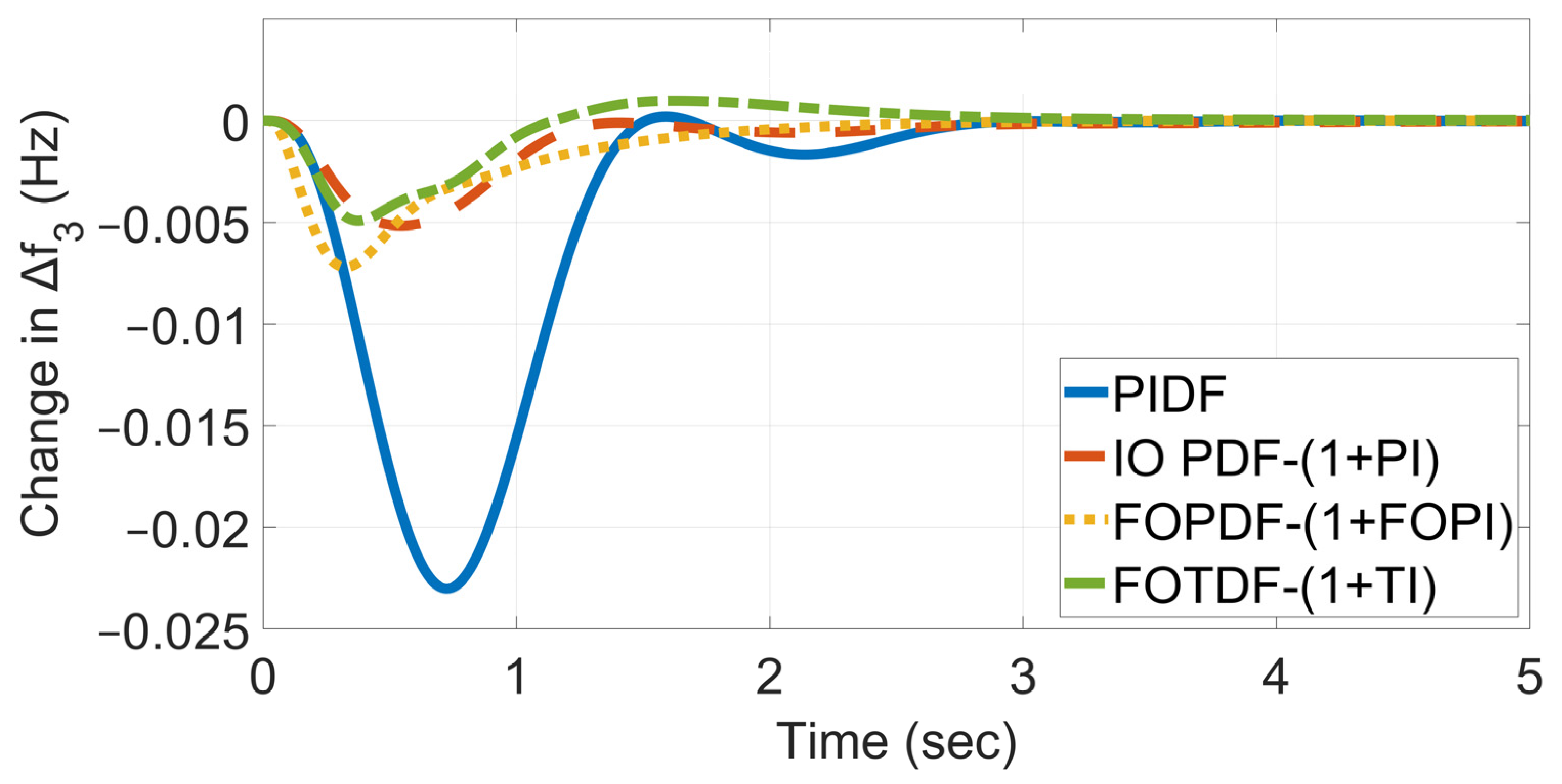
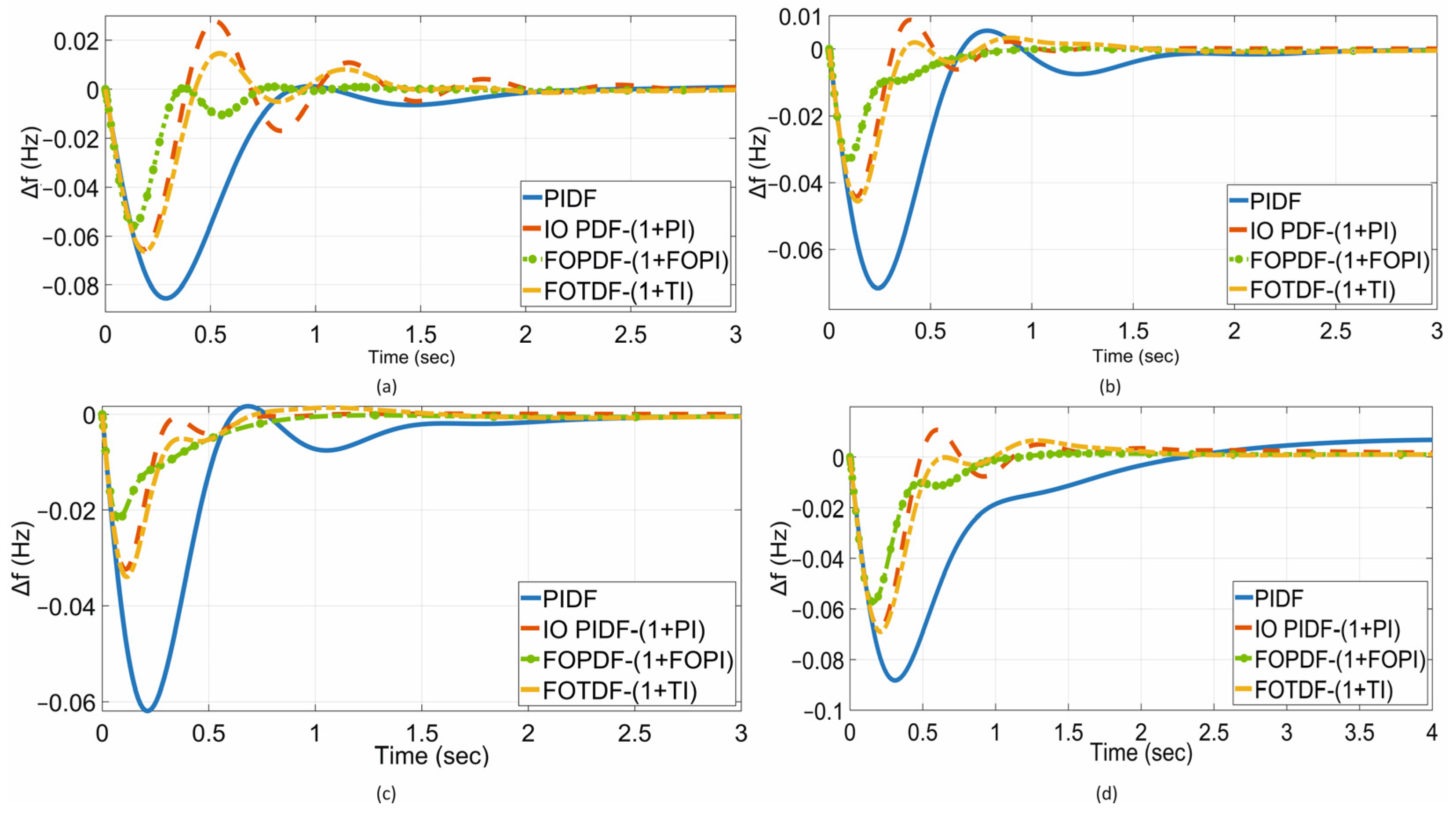
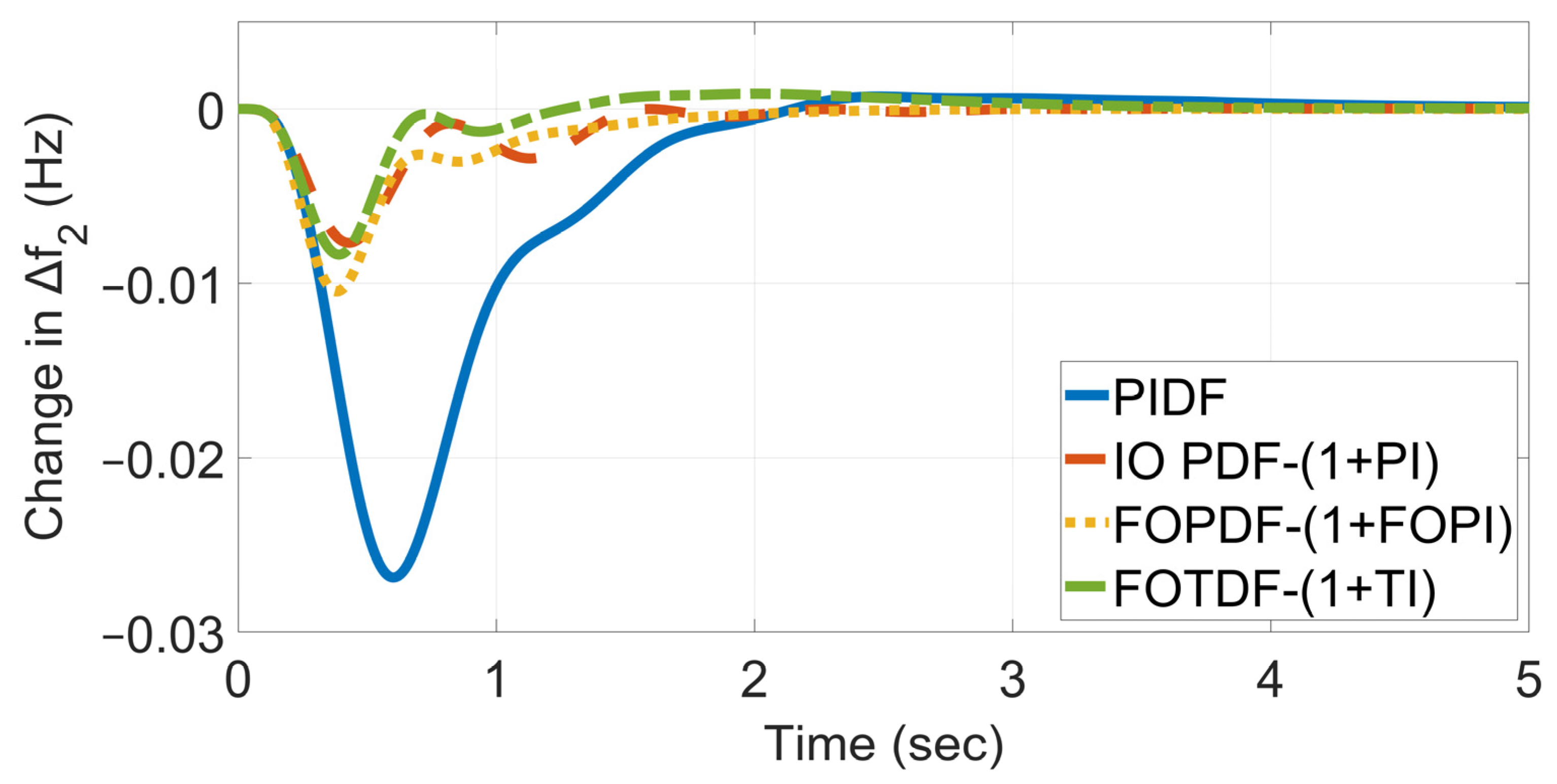
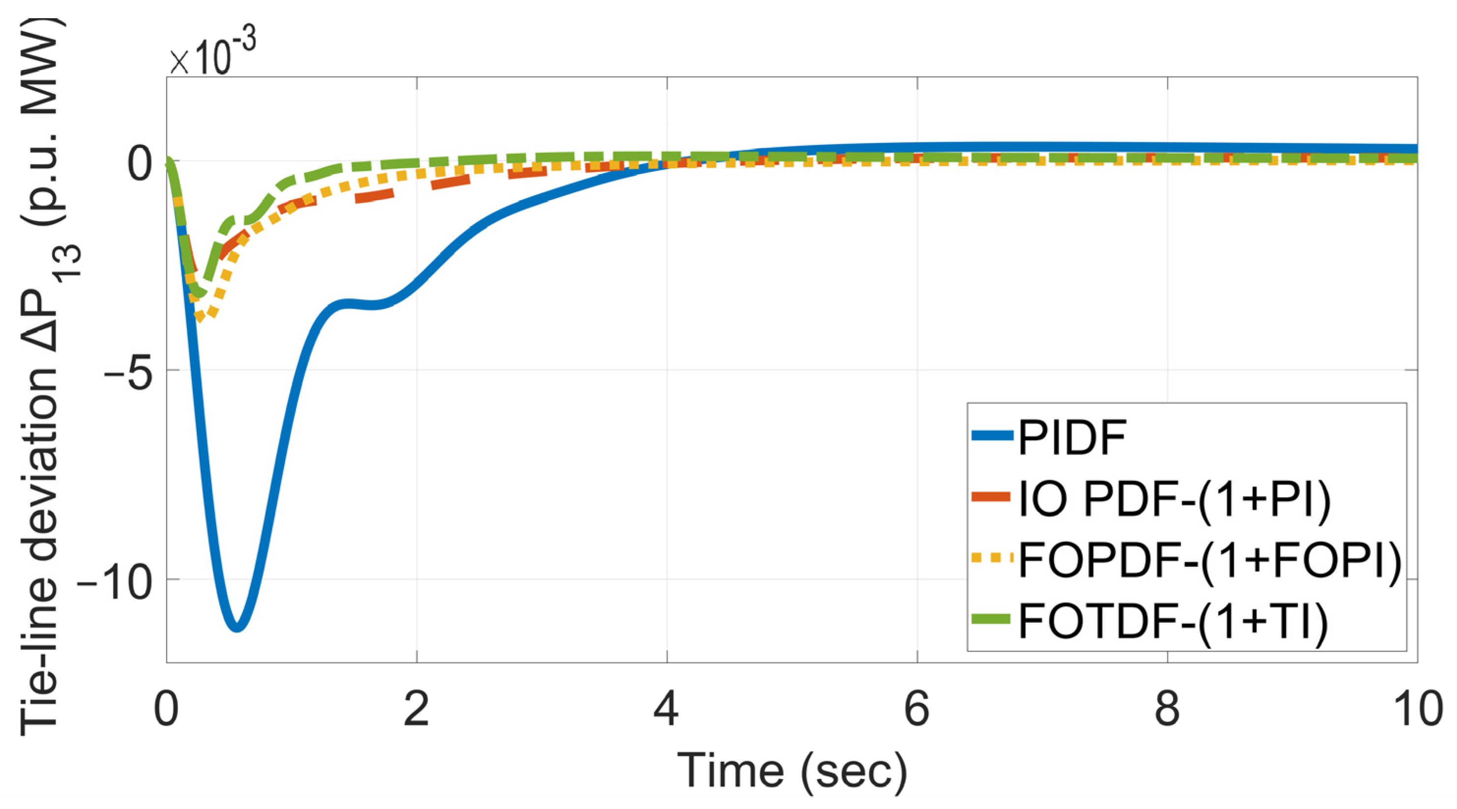
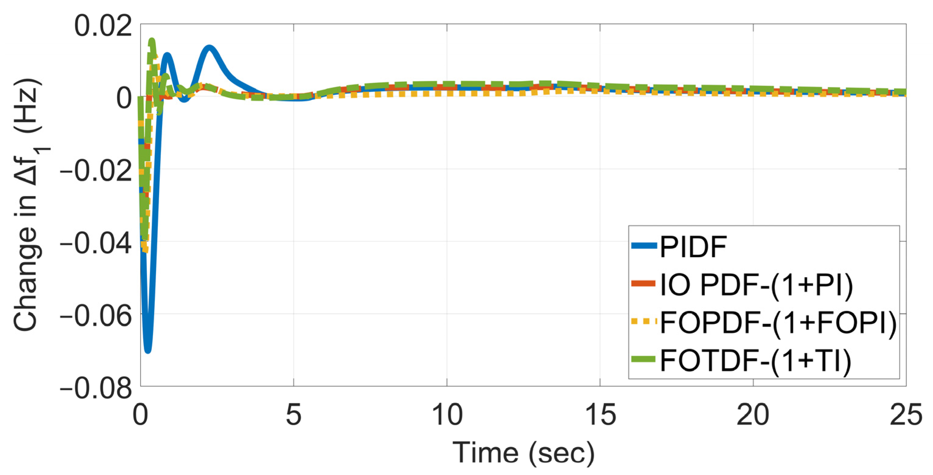
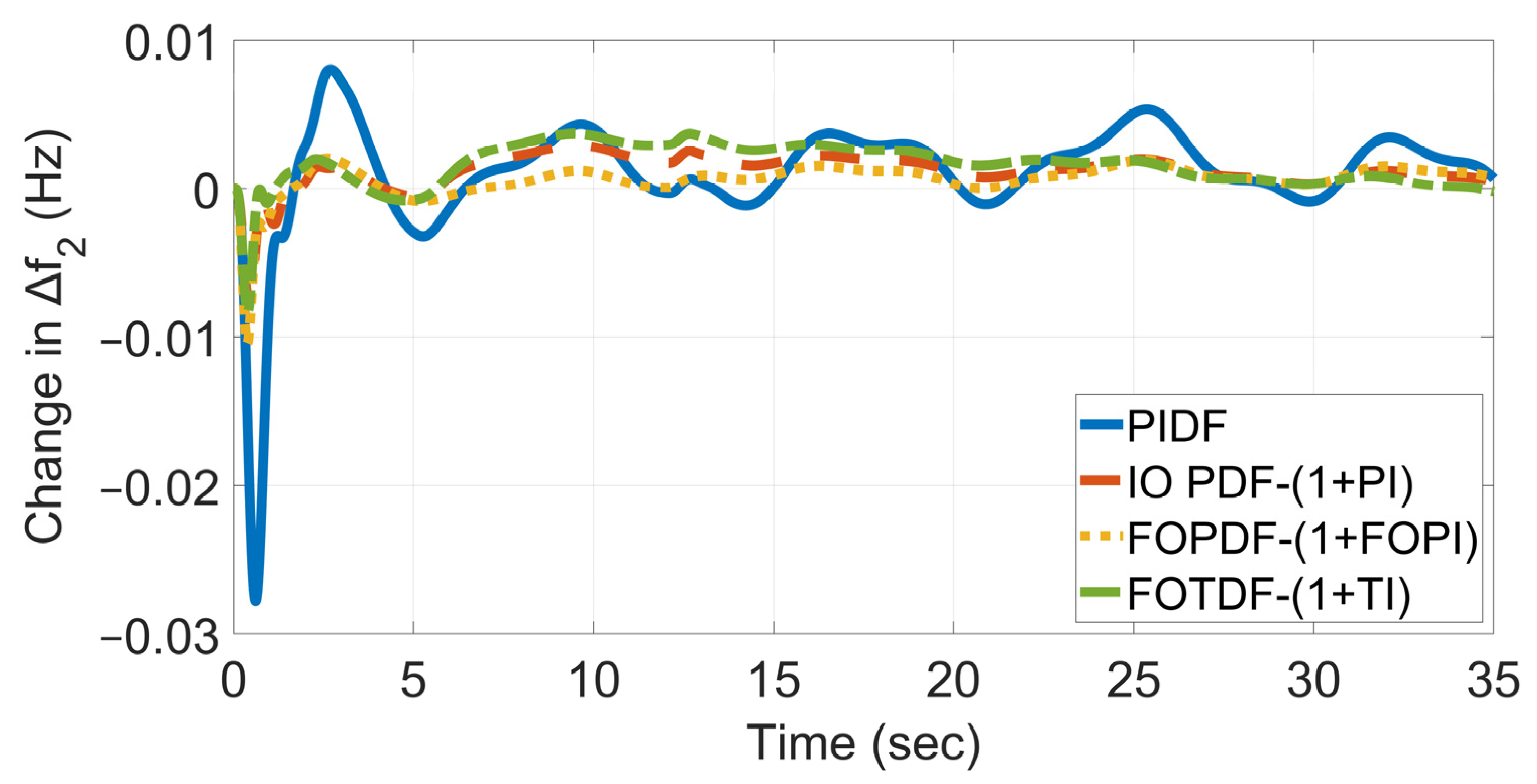
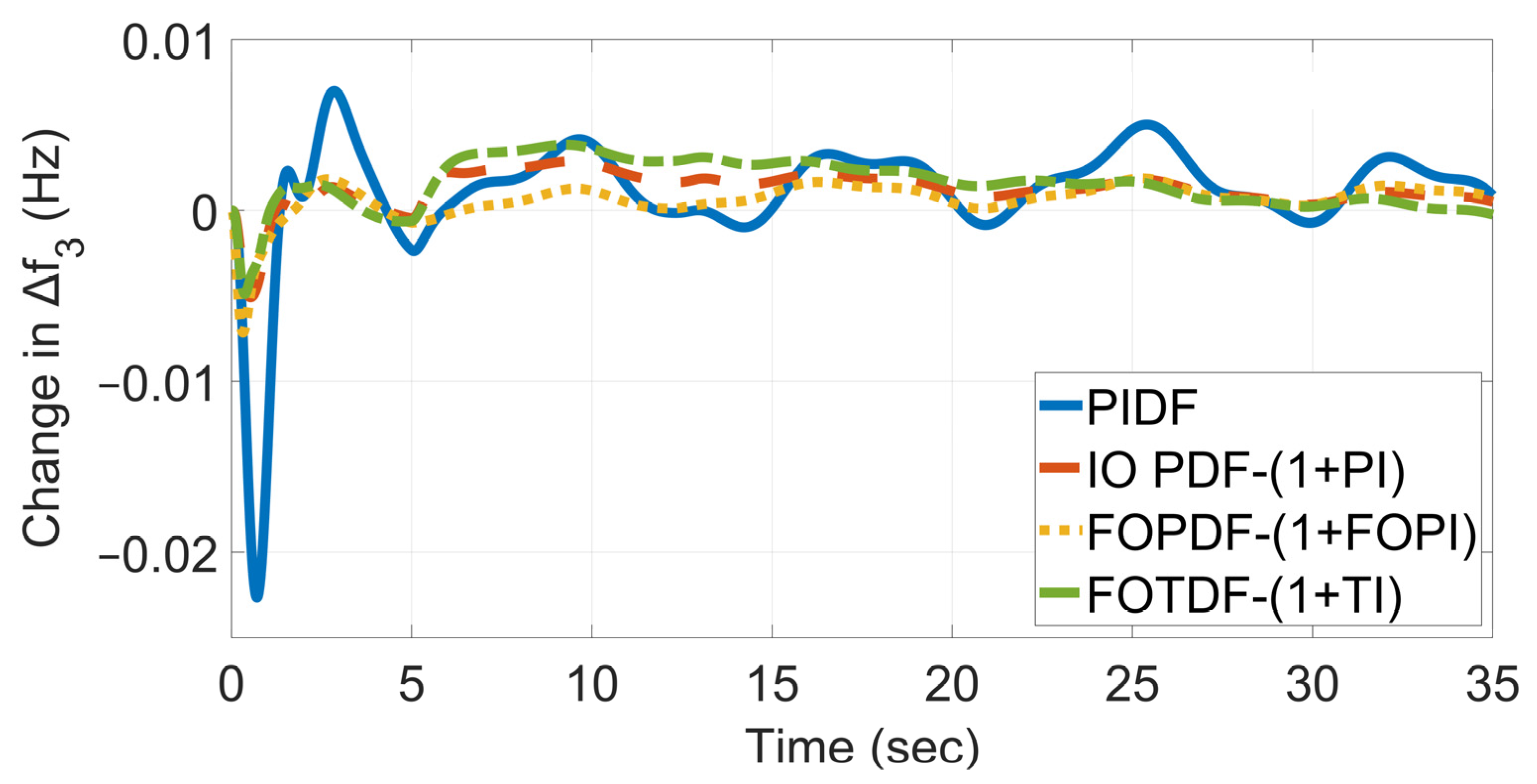
This study implemented a FOPDF (1+FOPI) controller in a single-area microgrid and three-area multi-source interconnected microgrids that incorporates bioenergy generation, RESs, and H-ESSs for frequency regulation. Firstly, the controller was tested in a single-area microgrid without RES penetration. The simulations revealed that the proposed controller improved the maximum overshoot by 41.18%, 96.42%, and 93.15% when compared to that of the PIDF, IO PDF-(1+PI), and FOTDF-(TI) controllers. Next, the proposed controller was evaluated in the three-area interconnected microgrids. The results showed that, compared to that of the PIDF and IO PDF-(1+PI) controllers, the proposed controller improved the settling time in area two by 38.29% and 17.75%. Following the introduction of a step and varied change in ORC-STTP, PV and sea wave generation in the form of disturbance, the proposed controller and the IO PDF-(1+PI) controller were able to effectively damp the disturbances in contrast to the PIDF and FOTDF-(1+TI) controllers. Subsequently, communication time delay was introduced in each area, and Gaussian noise was added to the control error in the first and second microgrids. The FOPDF-(1+FOPI) controller was more effective in suppressing the injected noise compared to the other three controllers. This improvement can be quantified in terms of the ITAE value, where the proposed controller had an ITAE value that was 45.4%, 14.52%, and 22.97% smaller than that of the other controllers. Finally, the performance of the proposed controller was tested for parameter uncertainties. The simulations revealed that the proposed controller is robust against unforeseen parameter changes.
Despite the higher complexity of the FOPDF-(1+FOPI) controller relative to the PIDF and IO PDF-(1+PI) controllers, the proposed controller offers enhanced time response characteristics and robustness. There are no inherent limitations in adopting the proposed controller aside from its computational demands.
Future work will assess the performance of the proposed controller’s via the incorporation of coupling between the LFC and AVR channels. Additionally, it will implement demand response mechanisms to contribute to frequency control.

Author Contributions

Conceptualization, I.M. (Ioannis Moschos) and C.P.; methodology, I.M. (Ioannis Moschos); software, I.M. (Ioannis Moschos); validation, I.M. (Ioannis Moschos), I.M. (Ioannis Mastoras) and C.P.; writing—original draft preparation, I.M. (Ioannis Moschos); writing—review and editing, I.M. (Ioannis Moschos), I.M. (Ioannis Mastoras) and C.P.; supervision, C.P. All authors have read and agreed to the published version of the manuscript.

Funding

This research received no external funding.

Data Availability Statement

Not applicable.

Conflicts of Interest

The authors declare no conflict of interest.

References

  1. Barik, A.K.; Das, D.C. Expeditious Frequency Control of Solar Photovoltaic/Biogas/Biodiesel Generator Based Isolated Renewable Microgrid Using Grasshopper Optimisation Algorithm. IET Renew. Power Gener. 2018, 12, 1659–1667. [Google Scholar] [CrossRef]
  2. Marques Lameirinhas, R.A.; Torres, J.P.N.; de Melo Cunha, J.P. A Photovoltaic Technology Review: History, Fundamentals and Applications. Energies 2022, 15, 1823. [Google Scholar] [CrossRef]
  3. Darwish, A.S.; Al-Dabbagh, R. Wind Energy State of the Art: Present and Future Technology Advancements. Renew. Energy Environ. Sustain. 2020, 5, 7. [Google Scholar] [CrossRef]
  4. ENTSO-E. Executive summary. In Inertia and Rate of Change of Frequency (RoCoF); ENTSO-E: Brussels, Belgium, 2020; Volume 17. [Google Scholar]
  5. Moschos, I.; Parisses, C. A 2DOF-TIDμcontroller for Combined Frequency and Voltage Regulation of Two Area Biorenewable Microgrids with RES and ESS. In Proceedings of the SyNERGY MED 2022–2nd International Conference on Energy Transition in the Mediterranean Area, Thessaloniki, Greece, 17–19 October 2022. [Google Scholar]
  6. Rasul, M.G.; Ault, C.; Sajjad, M. Bio-Gas Mixed Fuel Micro Gas Turbine Co-Generation for Meeting Power Demand in Australian Remote Areas. Energy Procedia 2015, 75, 1065–1071. [Google Scholar] [CrossRef]
  7. Muthu, D.; Venkatasubramanian, C.; Ramakrishnan, K.; Sasidhar, J. Production of Biogas from Wastes Blended with CowDung for Electricity Generation-A Case Study. In Proceedings of the IOP Conference Series: Earth and Environmental Science, Thanjavur, India, 17–18 March 2017; Volume 80. [Google Scholar]
  8. Nabi, M.N.; Akhter, M.S.; Shahadat, M.M.Z. Improvement of Engine Emissions with Conventional Diesel Fuel and Diesel-Biodiesel Blends. Bioresour. Technol. 2006, 97, 372–378. [Google Scholar] [CrossRef]
  9. Moschos, I.; Parisses, C.; Mastoras, I. A Suitable Controller for Frequency Control of Solar-Thermal/Biodiesel/Biomass/Micro-Hydro Generation of a Remote Community or Farm with Energy Storage. In Proceedings of the CEUR Workshop, Athens, Greece, 22–25 September 2022; Volume 3293. [Google Scholar]
  10. Agarwal, A.K. Biofuels (Alcohols and Biodiesel) Applications as Fuels for Internal Combustion Engines. Prog. Energy Combust. Sci. 2007, 33, 233–271. [Google Scholar] [CrossRef]
  11. Barik, A.K.; Das, D.C. Active Power Management of Isolated Renewable Microgrid Generating Power from Rooftop Solar Arrays, Sewage Waters and Solid Urban Wastes of a Smart City Using Salp Swarm Algorithm. In Proceedings of the International Conference on Technologies for Smart City Energy Security and Power: Smart Solutions for Smart Cities, ICSESP 2018, Bhubaneswar, India, 28–30 March 2018; Volume 2018. [Google Scholar]
  12. Arbon, I.M. Worldwide Use of Biomass in Power Generation and Combined Heat and Power Schemes. Proc. Inst. Mech. Eng. Part A J. Power Energy 2002, 216, 41–57. [Google Scholar] [CrossRef]
  13. Kundur, P. Power System Stability and Control by Prabha Kundur.Pdf; McGraw Hill: New York, NY, USA, 1994; ISBN 978-0-07-035958-1/978-0-07-063515-9. [Google Scholar]
  14. Elgerd, O.I.; Happ, H.H. Electric Energy Systems Theory: An Introduction. IEEE Trans. Syst. Man Cybern. 1972, 2, 296–297. [Google Scholar] [CrossRef]
  15. Moschos, I.; Parisses, C. A Distributed Order PID Controller for Load Frequency Control in a Two-Area Diverse-Unit Power System. In Proceedings of the 2021 4th International Conference on Electronics and Electrical Engineering Technology, Nanjing China, 3–5 December 2021; ACM: New York, NY, USA, 2021; pp. 128–133. [Google Scholar]
  16. Gulzar, M.M.; Rizvi, S.T.H.; Javed, M.Y.; Sibtain, D.; Salah ud Din, R. Mitigating the Load Frequency Fluctuations of Interconnected Power Systems Using Model Predictive Controller. Electronics 2019, 8, 156. [Google Scholar] [CrossRef]
  17. Gheisarnejad, M.; Khooban, M.H. Design an Optimal Fuzzy Fractional Proportional Integral Derivative Controller with Derivative Filter for Load Frequency Control in Power Systems. Trans. Inst. Meas. Control. 2019, 41, 2563–2581. [Google Scholar] [CrossRef]
  18. Babaei, F.; Safari, A.; Farrokhifar, M.; Younis, M.A.; Quteishat, A. Participation of Electric Vehicles in a Delay-Dependent Stability Analysis of LFC Considering Demand Response Control. Electronics 2022, 11, 3682. [Google Scholar] [CrossRef]
  19. Tripathy, S.; Debnath, M.K.; Kar, S.K. Optimal Design of PI/PD Dual Mode Controller Based on Quasi Opposition Based Learning for Power System Frequency Control. e-Prime-Adv. Electr. Eng. Electron. Energy 2023, 4, 100135. [Google Scholar] [CrossRef]
  20. Zishan, F.; Akbari, E.; Montoya, O.D.; Giral-Ramírez, D.A.; Molina-Cabrera, A. Efficient PID Control Design for Frequency Regulation in an Independent Microgrid Based on the Hybrid PSO-GSA Algorithm. Electronics 2022, 11, 3886. [Google Scholar] [CrossRef]
  21. Shayeghi, H.; Rahnama, A.; Mohajery, R.; Bizon, N.; Mazare, A.G.; Ionescu, L.M. Multi-Area Microgrid Load-Frequency Control Using Combined Fractional and Integer Order Master–Slave Controller Considering Electric Vehicle Aggregator Effects. Electronics 2022, 11, 3440. [Google Scholar] [CrossRef]
  22. Huynh, V.V.; Minh, B.L.N.; Amaefule, E.N.; Tran, A.T.; Tran, P.T. Highly Robust Observer Sliding Mode Based Frequency Control for Multi Area Power Systems with Renewable Power Plants. Electronics 2021, 10, 274. [Google Scholar] [CrossRef]
  23. Rabeh, R.; Ferfra, M.; Ezbakhe, A. Secondary Control of Islanded Microgrids Using Pievolutionary Algorithms under Uncertainties. Int. J. Renew. Energy Res. 2019, 9, 1827–1837. [Google Scholar]
  24. Lal, D.K.; Barisal, A.K. Load Frequency Control of AC Microgrid Interconnected Thermal Power System. IOP Conf. Ser. Mater. Sci. Eng. 2017, 225, 012090. [Google Scholar] [CrossRef]
  25. Murugesan, D.; Jagatheesan, K.; Shah, P.; Sekhar, R. Fractional Order PIλDμ Controller for Microgrid Power System Using Cohort Intelligence Optimization. Results Control. Optim. 2023, 11, 100218. [Google Scholar] [CrossRef]
  26. Jena, N.K.; Sahoo, S.; Naik, A.K.; Sahu, B.K.; Mohanty, K.B. Frequency Control of an AC Microgrid with Fractional Controller. In Proceedings of the Lecture Notes in Networks and Systems, Amsterdam, The Netherlands, 2–3 September 2021; Volume 151. [Google Scholar]
  27. Zaheeruddin; Singh, K. Intelligent Frequency Control in Microgrid: Fractional Order Fuzzy PID Controller. J. Intell. Fuzzy Syst. 2020, 39, 195–212. [Google Scholar] [CrossRef]
  28. Oshnoei, S.; Fathollahi, A.; Oshnoei, A.; Khooban, M.H. Microgrid Frequency Regulation Based on a Fractional Order Cascade Controller. Fractal Fract. 2023, 7, 343. [Google Scholar] [CrossRef]
  29. Annamraju, A.; Bhukya, L.; Nandiraju, S. Robust Frequency Control in a Standalone Microgrid: An Adaptive Fuzzy Based Fractional Order Cascade PD-PI Approach. Adv. Control. Appl. 2021, 3, e72. [Google Scholar] [CrossRef]
  30. Khooban, M.H.; Dragicevic, T.; Blaabjerg, F.; Delimar, M. Shipboard Microgrids: A Novel Approach to Load Frequency Control. IEEE Trans. Sustain. Energy 2018, 9, 843–852. [Google Scholar] [CrossRef]
  31. Tepljakov, A.; Petlenkov, E.; Belikov, J. FOMCON: Fractional-Order Modeling and Control Toolbox for MATLAB. In Proceedings of the 18th International Conference–Mixed Design of Integrated Circuits and Systems, MIXDES 2011, Gliwice, Poland, 16–18 June 2011. [Google Scholar]
  32. Colín-Cervantes, J.D.; Sánchez-López, C.; Ochoa-Montiel, R.; Torres-Muñoz, D.; Hernández-Mejía, C.M.; Sánchez-Gaspariano, L.A.; González-Hernández, H.G. Rational Approximations of Arbitrary Order: A Survey. Fractal Fract. 2021, 5, 267. [Google Scholar] [CrossRef]
  33. Naruei, I.; Keynia, F. A New Optimization Method Based on COOT Bird Natural Life Model. Expert Syst. Appl. 2021, 183, 115352. [Google Scholar] [CrossRef]
  34. Trojovska, E.; Dehghani, M.; Trojovsky, P. Zebra Optimization Algorithm: A New Bio-Inspired Optimization Algorithm for Solving Optimization Algorithm. IEEE Access 2022, 10, 49445–49473. [Google Scholar] [CrossRef]
Figure 1. Scheme of the isolated microgrid for LFC.
Electronics 12 04152 g001
Figure 2. Scheme of three-area interconnected microgrids for LFC.
Electronics 12 04152 g002
Figure 3. Block diagram of the FOPDF-(1+FOPI) controller.
Electronics 12 04152 g003
Figure 4. Block diagram of (a) PIDF and (b) IO PDF-(1+IOPI) controller.
Electronics 12 04152 g004
Figure 5. Block diagram of FOTDF-(1+TI) controller.
Electronics 12 04152 g005
Figure 6. Flowchart of coot optimization algorithm.
Electronics 12 04152 g006
Figure 7. Convergence curve of COA and ZOA.
Electronics 12 04152 g007
Figure 8. Dynamic response of the isolated microgrid for the ZOA and COA.
Electronics 12 04152 g008
Figure 9. Dynamic response of isolated microgrid: (a) Case 1, (b) Case 2, (c) Case 3, and (d) Case 4.
Electronics 12 04152 g009
Figure 10. Frequency deviation in area 1.
Electronics 12 04152 g010
Figure 11. Frequency deviation in area 2.
Electronics 12 04152 g011
Figure 12. Frequency deviation in area 3.
Electronics 12 04152 g012
Figure 13. Tie-line deviation between area 1 and 2.
Electronics 12 04152 g013
Figure 14. Tie-line deviation between areas 1 and 3.
Electronics 12 04152 g014
Figure 15. Frequency deviation in area 1 with solar energy penetration.
Electronics 12 04152 g015
Figure 16. Frequency deviation in area 2 with solar energy penetration.
Electronics 12 04152 g016
Figure 17. Frequency deviation in area 3 with solar energy penetration.
Electronics 12 04152 g017
Figure 18. Tie-line deviation between areas 1 and 3 with solar energy penetration.
Electronics 12 04152 g018
Figure 19. Power fluctuation of SWE.
Electronics 12 04152 g019
Figure 20. Frequency deviation in area 1 with solar and wave energy penetration.
Electronics 12 04152 g020
Figure 21. Frequency deviation in area 2 with solar and wave energy penetration.
Electronics 12 04152 g021
Figure 22. Frequency deviation in area 3 with solar and wave energy penetration.
Electronics 12 04152 g022
Figure 23. Tie-line deviation between areas 1 and 2 with solar and wave energy penetration.
Electronics 12 04152 g023
Figure 24. Tie-line deviation between areas 1 and 3 with solar and wave energy penetration.
Electronics 12 04152 g024
Figure 25. Frequency deviation in area 1 with RESs, delay, and noise injected in areas 1 and 2.
Electronics 12 04152 g025
Figure 26. Frequency deviation in area 2 with RESs, delay, and noise injected in areas 1 and 2.
Electronics 12 04152 g026
Figure 27. Frequency deviation in area 3 with RESs, delay and noise injected in areas 1 and 2.
Electronics 12 04152 g027
Table 1. Values and nomenclature used in modeling the microgrids.
ParameterValueDescription
fi-Frequency deviation in area i
Pij-Tie-line deviation between i and j microgrids
Di0.01Load damping constant of the i microgrid
Mi0.2Inertia constant of the i microgrid
Ri2Droop constant of the i microgrid
Bi0.51Frequency bias of the i microgrid
Tij0.080Synchronizing torque coefficient
KBESS, KFESS, KSMES, KSCES0.003, 0.01, 0.12, 0.7Gain of BESS, FESS, SMES, SCES
TBESS, TFESS, TSMES, TSCES0.1, 0.1, 0.03, 0.9Time constant of BESS, FESS, SMES, SCES
aij−1Power transfer ratio
KLFR, TLFR5, 0.42Gain and time constant of LFR
KORC0.95Gain of ORC
THX, TST0.1, 0.3Time constants of heat exchanger, turbine of STPP
TSWG, TSWT0.5, 4Time constants of SWE
Tp2, Tp10.041, 0.6Time constants of WPP
Kp2, KPC, Kp31.25, 1.4, 0.8Gains of WPP
TGG, TGT0.05, 0.1Time constants of geothermal governor and turbine
KPV, TPV1, 1.8Gain and time constant of PV
KVA, KVE1, 1Gains of BDEG
TVA, TVE0.055, 0.5Valve actuator, engine time constants of BDEG
TMG, TRS, TRH, THT0.2, 5, 28.75, 1Time constants of MHTG
bB, XC, YC0.05, 0.6, 1Valve actuator, lead and lag time of BGTG
TCR, TBG, TBT0.01, 0.23, 0.2Combustion reaction delay, biogas delay, discharge time constants of BGTG
TBSG, TBCT0.08, 0.3Speed governor and turbine time constant of BCHP
KR, TR0.3, 10Gain and reheat time constant of BCHP
Table 2. Statistical results and time domain characteristics of the COA and ZOA.
COAZOA
Minimum0.01290.0132
Average0.01790.0312
Standard deviation0.00910.0193
Settling time0.69930.9561
Maximum overshoot0.00100.0026
Maximum undershoot−0.0558−0.0552
Table 3. Optimal controller gains for the isolated microgrid with no solar, wind, and wave availability.
PIDF
KpKiKdN
2.84440.2372485.9112
IO PDF-(1+PI)
Kp1KdNKp2Ki
41.26525000.244
FOPDF-(1+FOPI)
Kp1KdNKp2Kiml
3.9990.8263480.1940.48503.99841.30570.8158
FOTDF-(1+TI)
Kt1KdNKt2Kin1n2m
3.89470.71835003.71030.00223.106821.0928
Table 4. Transient response characteristics for the isolated microgrid.
ControllerCase 1: KMHTG = 0.35, KBDEG = 0.35, KBCHP = 0.3
OvershootUndershootSettling TimeITAE
PIDF0.0017−0.08541.92790.2025
IO PDF-(1+PI)0.0279−0.06551.93250.0585
FOPDF-(1+FOPI)0.0010−0.05580.69930.0129
FOTDF-(1+TI)0.0146−0.06631.34850.0183
Case 2: KMHTG = 0.25, KBDEG = 0.75, KBCHP = 0
OvershootUndershootSettling timeITAE
PIDF0.0055−0.07161.62250.0746
IO PDF-(1+PI)0.0089−0.04430.92050.0178
FOPDF-(1+FOPI)5.5736 × 10⁻⁶−0.03320.69350.0426
FOTDF-(1+TI)0.0033−0.04561.0550.0469
Case 3: KMHTG = 0, KBDEG = 0.9, KBCHP = 0.1
OvershootUndershootSettling timeITAE
PIDF0.0017−0.06191.49860.0271
IO PDF-(1+PI)1.3167 × 10⁻⁴−0.03250.62310.0051
FOPDF-(1+FOPI)0−0.02190.71830.0519
FOTDF-(1+TI)0.0014−0.03390.62200.0555
Case 4: KMHTG = 0.2, KBDEG = 0, KBCHP = 0.8
OvershootUndershootSettling timeITAE
PIDF0.0069−0.08838.91120.2821
IO PDF-(1+PI)0.0109−0.06783.52100.0655
FOPDF-(1+FOPI)0.0014−0.05730.92220.0520
FOTDF-(1+TI)0.0066−0.0692.05240.0552
Table 5. Controller parameters of the interconnected microgrids with no solar and wave availability.
Optimal Values of Controllers Parameters
Area 1Area 2Area 3
PIDF
Kp = 4Kp = 3.845Kp = 0.648
Ki = 4Ki = 3.534Ki = 0.131
Kd = 0.926Kd = 3.157Kd = 0.613
N = 50N = 458.79N = 136.92
IO PDF-(1+PI)
Kp1 = 4Kp1 = 2.014Kp1 = 0.381
Kd = 0.609Kd = 2.321Kd = 0.312
N = 264.28N = 341.01N = 128.12
Kp2 = 4Kp2 = 0.448Kp2 = 0.3
Ki = 4Ki = 0.957Ki = 0.339
FOPDF-(1+FOPI)
Kp1 = 4Kp1 = 0.467Kp1 = 1.983
Kd = 1.516Kd = 1.506Kd = 3.947
N = 367.01N = 387.09N = 496.89
Kp2 = 0.956Kp2 = 1.764Kp2 = 0.188
Ki = 4Ki = 1.788Ki = 2.009
λ = 0.9λ = 1.203λ = 1.105
m = 0.906m = 1.236m = 0.039
FOTDF-(1+TI)
Kt1 = 4Kt1 = 1.6197Kt1 = 0.0728
n1 = 4n1 = 3.2395n1 = 2.0544
Kd = 1.926Kd = 1.8508Kd = 0.5527
N = 500N = 254.4703N = 356.0112
m = 0.9428m = 1.298m = 1.2489
Kt2 = 4Kt2 = 0.0384Kt2 = 0.0937
n2 = 2n2 = 2.7779n2 = 3.9867
Ki = 3.997Ki = 4Ki = 0.2971
Table 6. Time domain characteristics of the interconnected microgrids with no solar and wave availability.
PIDFIO PDF-(1+PI)FOPDF-(1+FOPI)FOTDF-(1+TI)
ΙΤAΕ0.2190.04910.02280.0501
Settling time
Δf13.07940.43610.64271.3464
Δf21.70211.27721.05040.6002
Δf31.33650.99271.08220.8666
Maximum overshoot
Δf10.01130.00480.01110.0154
Δf26.582 × 10−42.307 × 10−57.9103 × 10−68.7100 × 10⁻⁴
Δf31.348 × 10−48.117 × 10−61.3608 × 10−69.8343 × 10⁻⁴
Maximum undershoot
Δf1−0.0702−0.0356−0.0432−0.0397
Δf2−0.0282−0.0077−0.0105−0.0084
Δf3−0.0232−0.0052−0.0072−0.0049
Table 7. ITAE value for interconnected microgrids with solar penetration.
Controller
PIDFIO PDF-(1+PI)FOPDF-(1+FOPI)FOTDF-(1+TI)
ITAE2.50212.44601.39203.2821
Table 8. ITAE value for interconnected microgrids with solar and sea wave penetration.
Controller
PIDFIO PDF-(1+PI)FOPDF-(1+FOPI)FOTDF-(1+TI)
ΙΤAΕ4.15943.12582.293.6372
Table 9. ITAE value for interconnected microgrids with RESs, time delay, and noise.
Controller
PIDFIO PDF-(1+PI)FOPDF-(1+FOPI)FOTDF-(1+TI)
ΙΤAΕ5.69123.63513.10724.0335
Table 10. Evaluation of robustness against parameter uncertainties for Δf1.
Parameter VariationMax. OvershootMin. OvershootSettling TimeITAE
Nominal-0.0111−0.04320.64270.0228
TGG+25%0.0154−0.04541.07070.0235
−25%0.0080−0.04070.73220.0228
TRS+25%0.0136−0.04470.64780.0230
−25%0.0089−0.04170.63600.0239
TVA+25%0.0122−0.04370.64710.0229
−25%0.0098−0.04240.64750.0228
TSCES+25%0.0111−0.04320.64250.0229
−25%0.0111−0.04320.64280.0229
TBSG+25%0.0116−0.04340.65080.0229
−25%0.0104−0.04280.64540.0228
TCR+25%0.0110−0.04310.64400.0228
−25%0.0112−0.04320.64510.0228
Disclaimer/Publisher’s Note: The statements, opinions and data contained in all publications are solely those of the individual author(s) and contributor(s) and not of MDPI and/or the editor(s). MDPI and/or the editor(s) disclaim responsibility for any injury to people or property resulting from any ideas, methods, instructions or products referred to in the content.

