
A Distributed Conflict-Free Task Allocation Method for Multi-AGV Systems

Abstract
:1. Background Introduction
2. Control Law for Maintaining Connectivity
2.1. Graph Theory Knowledge
2.2. Controller Design
3. Task Allocation
3.1. Task Bundles Construction
- ①
- .
- ②
- Calculate the reward . If task is already in the task bundle, . When , .
- ③
- Calculate and use to record the task label corresponding to the maximum value.
- ④
- where is the reward for completing the task in the task bundle.
- ⑤
- Repeat ①, ②, ③, ④ until no more tasks can be added.
3.2. Conflicts Resolution
- ①
- Send the column vectors and to its neighbor AGVs, and receive the and , .
- ②
- Update : , and deposit the corresponding AGV label into .
- ③
- For , if , set , and if changes from 1 to 0, task and its subsequent tasks are cleared from the task bundle and update , and at the same time; otherwise, if and , set and .
- ④
- Repeat ①, ②, ③ until and no longer change.
4. Examples
4.1. Task Allocation
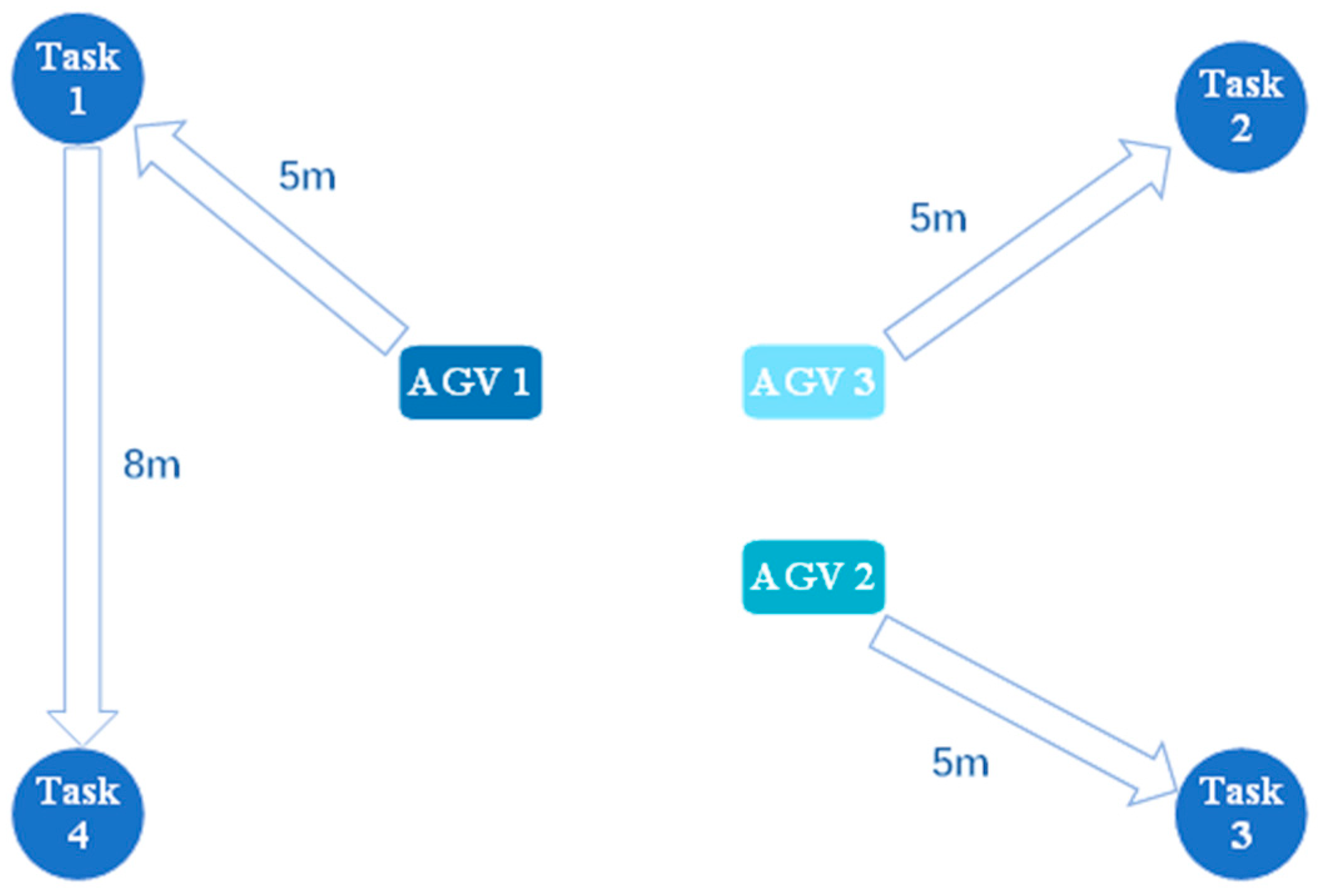
4.1.1. Three AGVs
- ①
- .
- ②
- ①
- .
- ②
- ①
- .
- ②
- ①
- .
- ②
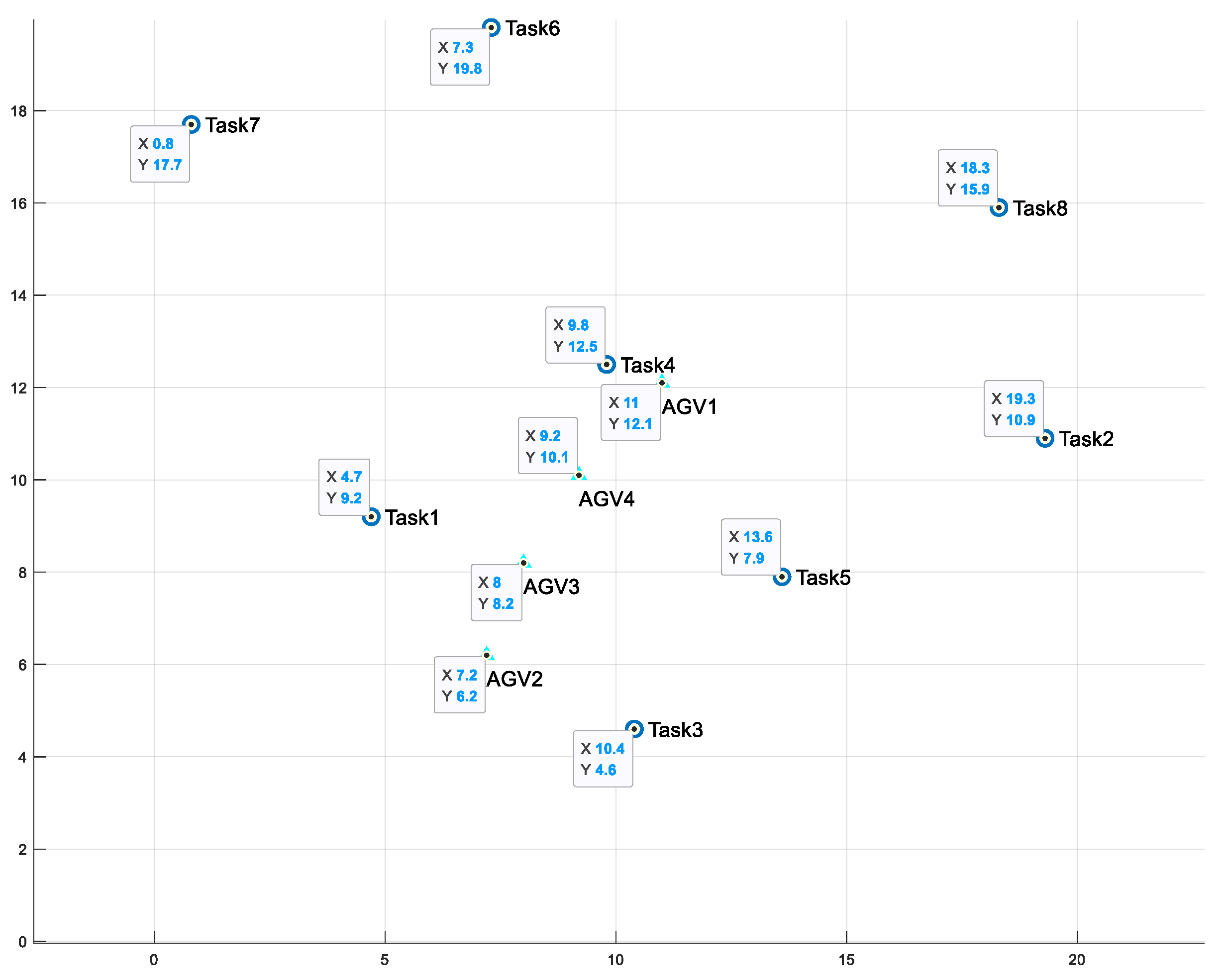
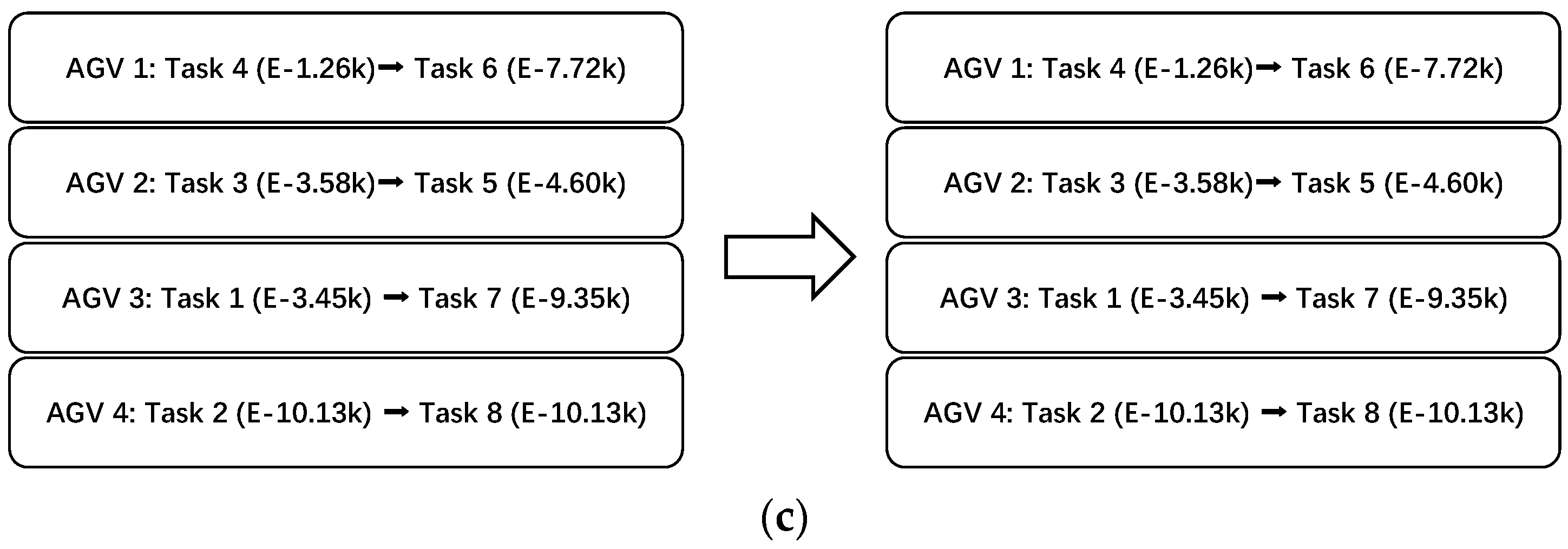
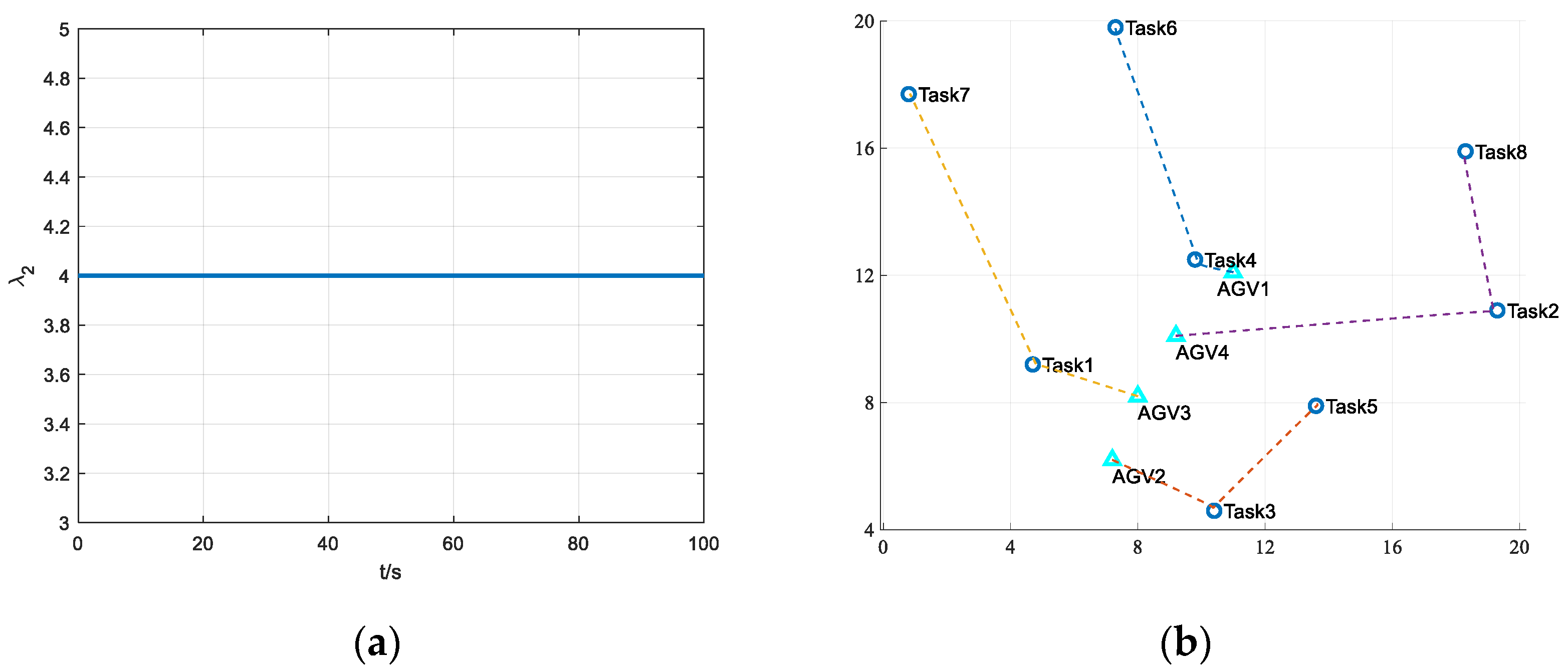
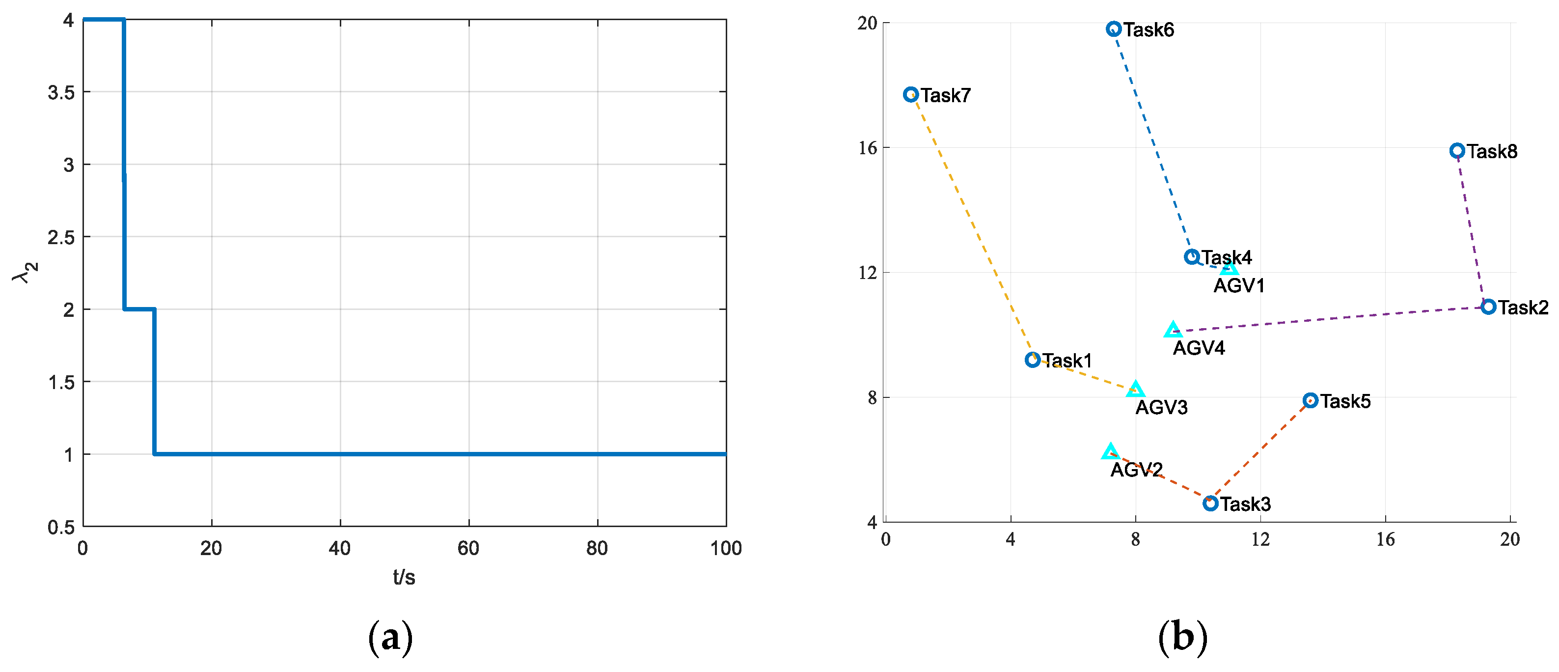
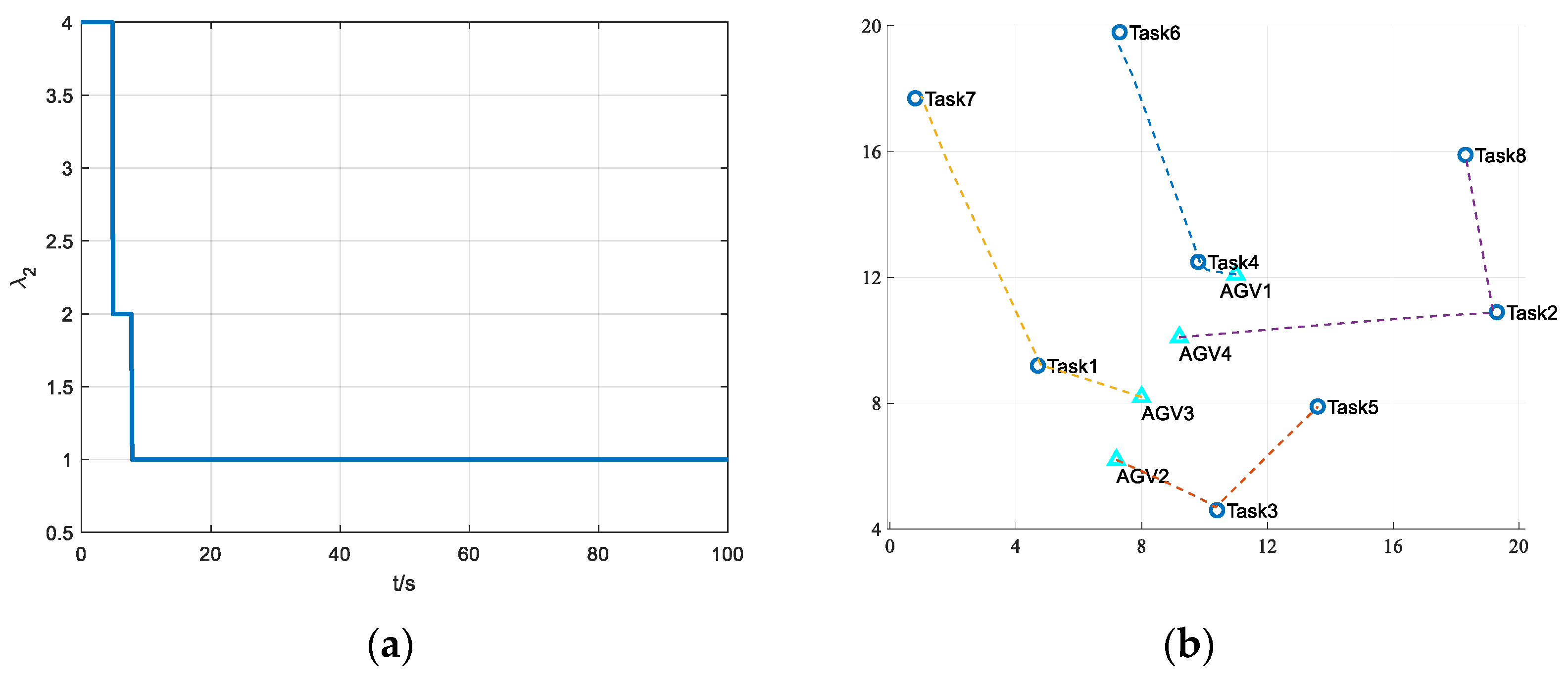
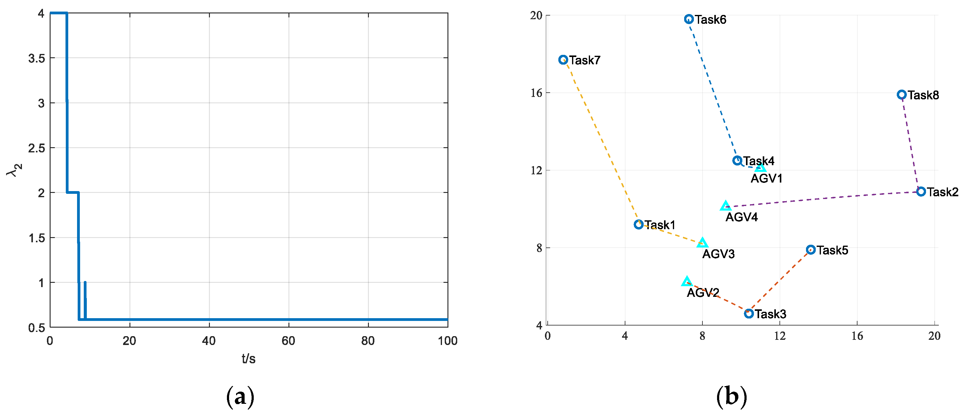
4.1.2. Multiple AGVs
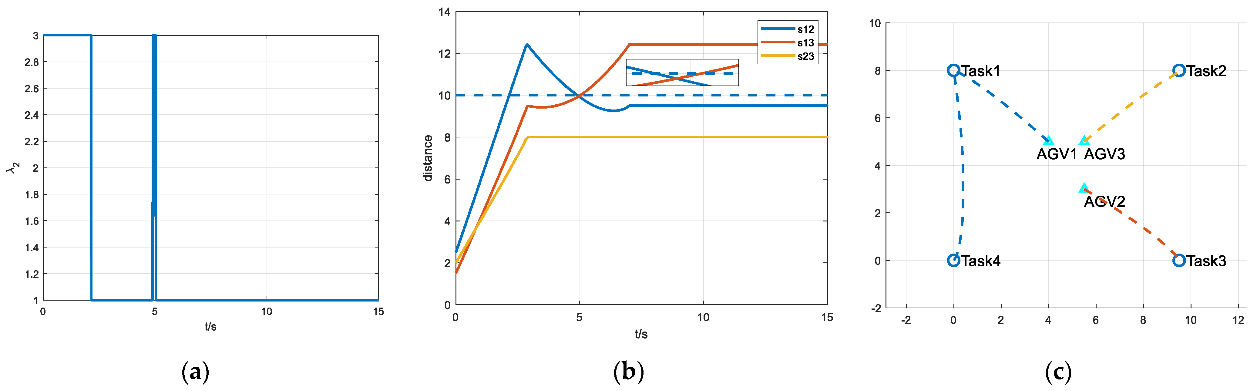
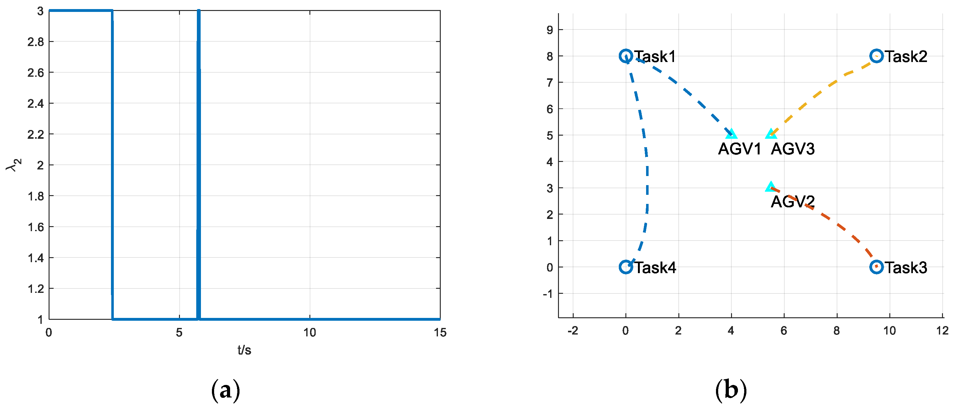
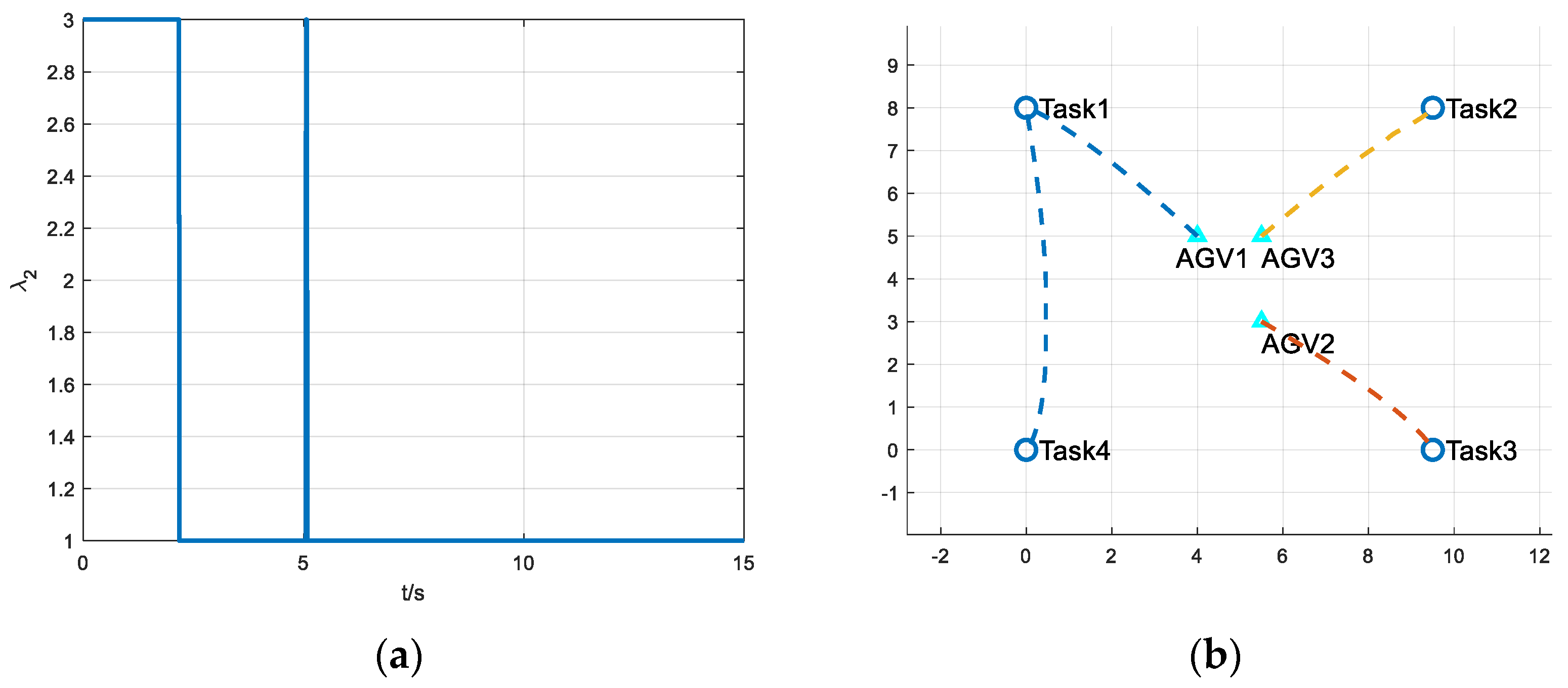
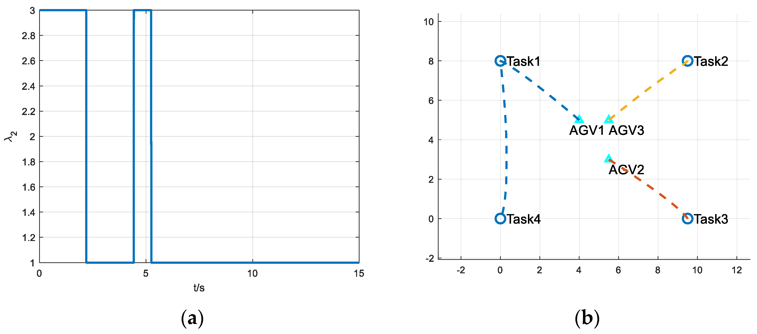
4.2. Task Execution
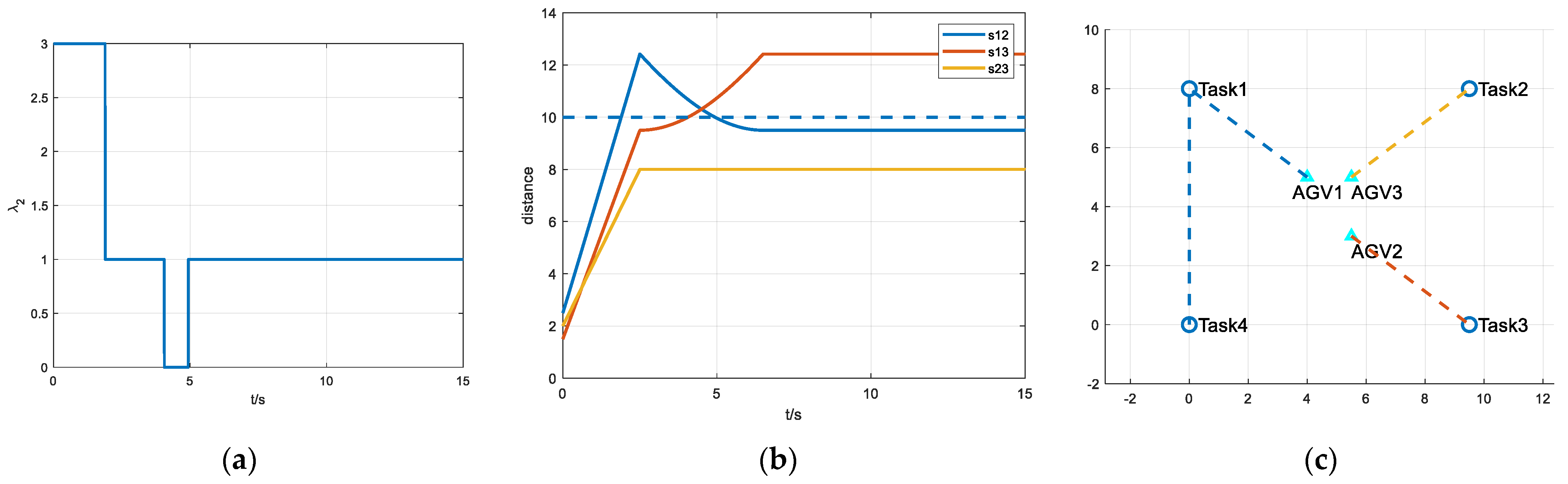
4.2.1. Three AGVs
4.2.2. Multiple AGVs
5. Conclusions
Author Contributions
Funding
Data Availability Statement
Conflicts of Interest
References
- Kumar, M.V.S.; Janardhana, R.; Rao, C.S.P. Simultaneous scheduling of machines and vehicles in an FMS environment with alternative routing. Int. J. Adv. Manuf. Technol. 2011, 53, 339–351. [Google Scholar] [CrossRef]
- Rashidi, H.; Tsang, E.P.K. A complete and an incomplete algorithm for automated guided vehicle scheduling in container terminals. Comput. Math. Appl. 2011, 61, 630–641. [Google Scholar] [CrossRef]
- Jerald, J.; Asokan, P.; Prabaharan, G.; Saravanan, R. Allocation optimisation of flexible manufacturing systems using particle swarm optimisation algorithm. Int. J. Adv. Manuf. Technol. 2005, 25, 964–971. [Google Scholar] [CrossRef]
- Udhayakumar, P.; Kumanan, S. Task scheduling of AGV in FMS using non-traditional optimization techniques. Int. J. Simul. Model. 2010, 9, 28–39. [Google Scholar] [CrossRef]
- Liu, Y.; Ji, S.; Su, Z.; Guo, D. Multi-objective AGV scheduling in an automatic sorting system of an unmanned (intelligent) warehouse by using two adaptive genetic algorithms and a multi-adaptive genetic algorithm. PLoS ONE 2019, 14, e0226161. [Google Scholar] [CrossRef] [PubMed]
- Michael, N.; Zavlanos, M.M.; Kumar, V.; Pappas, G.J. Distributed multi-robot task assignment and formation control. In Proceedings of the 2008 IEEE International Conference on Robotics and Automation, Pasadena, CA, USA, 19–23 May 2008; pp. 128–133. [Google Scholar]
- Maoudj, A.; Bouzouia, B.; Hentout, A.; Kouider, A.; Toumi, R. Distributed multi-agent approach based on priority rules and genetic algorithm for tasks scheduling in multi-robot cells. In Proceedings of the IECON 2016—42nd Annual Conference of the IEEE Industrial Electronics Society, Florence, Italy, 23–26 October 2016; pp. 692–697. [Google Scholar]
- Housseyni, W.; Mosbahi, O.; Khalgui, M.; Li, Z.; Yin, L.; Chetto, M. Multiagent architecture for distributed adaptive scheduling of reconfigurable real-time tasks with energy harvesting constraints. IEEE Access 2018, 6, 2068–2084. [Google Scholar] [CrossRef]
- Sabattini, L.; Chopra, N.; Secchi, C. Decentralized connectivity maintenance for cooperative control of mobile robotic systems. Int. J. Robot. Res. 2013, 32, 1411–1423. [Google Scholar] [CrossRef]
- Yang, P.; Freeman, R.A.; Gordon, G.J.; Lynch, K.M.; Srinivasa, S.S.; Sukthankar, R. Decentralized estimation and control of graph connectivity for mobile sensor networks. Automatic 2010, 46, 390–396. [Google Scholar] [CrossRef]
- Khateri, K.; Pourgholi, M.; Montazeri, M.; Sabattini, L. A Comparison between decentralized local and global methods for connectivity maintenance of multi-robot networks. IEEE Rob. Autom. Lett. 2019, 4, 633–640. [Google Scholar] [CrossRef]
- Liu, C.; Zhang, Z. Towards a robust FANET: Distributed node importance estimation-based connectivity maintenance for UAV swarms. Ad. Hoc. Netw. 2022, 125, 102734. [Google Scholar] [CrossRef]
- Gasparri, A.; Sabattini, L.; Ulivi, G. Bounded control law for global connectivity maintenance in cooperative multirobot systems. IEEE Trans. Robot. 2017, 33, 700–717. [Google Scholar] [CrossRef]
- Karkoub, M.; Atinc, G.; Stipanovic, D.; Voulgaris, P.; Hwang, A. Trajectory tracking control of unicycle robots with collision avoidance and connectivity maintenance. J. Intell. Robot. Syst. 2019, 96, 331–343. [Google Scholar] [CrossRef]
- Fang, H.; Wei, Y.; Chen, J.; Xin, B. Flocking of second-order multiagent systems with connectivity preservation based on algebraic connectivity estimation. IEEE Trans. Cybern. 2017, 47, 1067–1077. [Google Scholar] [CrossRef] [PubMed]
- Zavlanos, M.M.; Pappas, G.J. Controlling connectivity of dynamic graphs. In Proceedings of the 44th IEEE Conference on Decision and Control, Seville, Spain, 15 December 2005; pp. 6388–6393. [Google Scholar]
- Choi, H.-L.; Brunet, L.; How, J.P. Consensus-based decentralized auctions for robust task allocation. IEEE Trans. Robot. 2009, 25, 912–926. [Google Scholar] [CrossRef]
- Johnson, L.B.; Choi, H.L.; Ponda, S.S.; How, J.P. Decentralized task allocation using local information consistency assumptions. J. Aerosp. Comput. Inf. Commun. 2017, 14, 103–122. [Google Scholar] [CrossRef]
- Kawakami, H.; Namerikawa, T. Cooperative target-capturing strategy for multi-vehicle systems with dynamic network topology. In Proceedings of the American Control Conference, St. Louis, MI, USA, 10–12 June 2009; pp. 635–640. [Google Scholar]
- Rafiee, M.; Bayen, A. Optimal network topology design in multi-agent systems for efficient average consensus. In Proceedings of the IEEE Conference on Decision and Control, Atlanta, GE, USA, 15–17 December 2010; pp. 3877–3883. [Google Scholar]
- Zavlanos, M.M.; Egerstedt, M.B.; Pappas, G.J. Graph-theoretic connectivity control of mobile robot networks. Proc. IEEE 2011, 99, 1525–1540. [Google Scholar] [CrossRef]


| Task 1 | Task 2 | Task 3 | Task 4 | |
|---|---|---|---|---|
| AGV 1 | 5 | 6.265 | 7.433 | 6.403 |
| AGV 2 | 7.433 | 6.403 | 5 | 6.265 |
| AGV 3 | 6.265 | 5 | 6.403 | 7.433 |
| (a) The results after stage one ends. | ||||
| AGV 1 | ||||
| AGV 2 | ||||
| AGV 3 | ||||
| (b) The results after stage two ends. | ||||
| AGV 1 | ||||
| AGV 2 | ||||
| AGV 3 | ||||
| AGV 1 | ||||
| AGV 2 | ||||
| AGV 3 |
| (a) The distances between AGVs and task points. | ||||||||
| AGV/TASK | 1 | 2 | 3 | 4 | 5 | 6 | 7 | 8 |
| 1 | 6.94 | 8.39 | 7.52 | 1.26 | 4.94 | 8.54 | 11.64 | 8.23 |
| 2 | 3.91 | 12.98 | 3.58 | 6.82 | 6.62 | 13.60 | 13.16 | 14.74 |
| 3 | 3.45 | 11.62 | 4.33 | 4.66 | 5.61 | 11.62 | 11.92 | 12.86 |
| 4 | 4.59 | 10.13 | 5.63 | 2.47 | 4.92 | 9.88 | 11.33 | 10.79 |
| (b) The distances between AGVs. | ||||||||
| TASK/TASK | 1 | 2 | 3 | 4 | 5 | 6 | 7 | 8 |
| 1 | \ | 14.70 | 7.32 | 6.07 | 8.99 | 10.91 | 9.35 | 15.16 |
| 2 | 14.70 | \ | 10.90 | 9.63 | 6.44 | 14.94 | 19.71 | 5.10 |
| 3 | 7.32 | 10.90 | \ | 7.92 | 4.60 | 15.51 | 16.24 | 13.79 |
| 4 | 6.07 | 9.63 | 7.92 | \ | 5.97 | 7.72 | 10.39 | 9.15 |
| 5 | 8.99 | 6.44 | 4.60 | 5.97 | \ | 13.46 | 16.12 | 9.28 |
| 6 | 10.91 | 14.94 | 15.51 | 7.72 | 13.46 | \ | 6.83 | 11.67 |
| 7 | 9.35 | 19.71 | 16.24 | 10.39 | 16.12 | 6.83 | \ | 17.59 |
| 8 | 15.16 | 5.10 | 13.79 | 9.15 | 9.28 | 11.67 | 17.59 | \ |
Disclaimer/Publisher’s Note: The statements, opinions and data contained in all publications are solely those of the individual author(s) and contributor(s) and not of MDPI and/or the editor(s). MDPI and/or the editor(s) disclaim responsibility for any injury to people or property resulting from any ideas, methods, instructions or products referred to in the content. |
© 2023 by the authors. Licensee MDPI, Basel, Switzerland. This article is an open access article distributed under the terms and conditions of the Creative Commons Attribution (CC BY) license (https://creativecommons.org/licenses/by/4.0/).
Share and Cite
Guo, Q.; Yao, H.; Liu, Y.; Tang, Z.; Zhang, X.; Li, N. A Distributed Conflict-Free Task Allocation Method for Multi-AGV Systems. Electronics 2023, 12, 3877. https://doi.org/10.3390/electronics12183877
Guo Q, Yao H, Liu Y, Tang Z, Zhang X, Li N. A Distributed Conflict-Free Task Allocation Method for Multi-AGV Systems. Electronics. 2023; 12(18):3877. https://doi.org/10.3390/electronics12183877
Chicago/Turabian StyleGuo, Qiang, Haiyan Yao, Yi Liu, Zhipeng Tang, Xufeng Zhang, and Ning Li. 2023. "A Distributed Conflict-Free Task Allocation Method for Multi-AGV Systems" Electronics 12, no. 18: 3877. https://doi.org/10.3390/electronics12183877
APA StyleGuo, Q., Yao, H., Liu, Y., Tang, Z., Zhang, X., & Li, N. (2023). A Distributed Conflict-Free Task Allocation Method for Multi-AGV Systems. Electronics, 12(18), 3877. https://doi.org/10.3390/electronics12183877