Article

GR(1)-Guided Deep Reinforcement Learning for Multi-Task Motion Planning under a Stochastic Environment

1
School of Computer Science and Artificial Intelligence, Changzhou University, Changzhou 213100, China
2
Department of Electronics and Computer Science, University of Southampton, Southampton SO17 1BJ, UK
*
Author to whom correspondence should be addressed.
Electronics 2022, 11(22), 3716; https://doi.org/10.3390/electronics11223716
Submission received: 27 October 2022 / Revised: 8 November 2022 / Accepted: 10 November 2022 / Published: 13 November 2022
(This article belongs to the Special Issue Recent Advances in Multi-Agent System)

Abstract

:
Motion planning has been used in robotics research to make movement decisions under certain movement constraints. Deep Reinforcement Learning (DRL) approaches have been applied to the cases of motion planning with continuous state representations. However, current DRL approaches suffer from reward sparsity and overestimation issues. It is also challenging to train the agents to deal with complex task specifications under deep neural network approximations. This paper considers one of the fragments of Linear Temporal Logic (LTL), Generalized Reactivity of rank 1 (GR(1)), as a high-level reactive temporal logic to guide robots in learning efficient movement strategies under a stochastic environment. We first use the synthesized strategy of GR(1) to construct a potential-based reward machine, to which we save the experiences per state. We integrate GR(1) with DQN, double DQN and dueling double DQN. We also observe that the synthesized strategies of GR(1) could be in the form of directed cyclic graphs. We develop a topological-sort-based reward-shaping approach to calculate the potential values of the reward machine, based on which we use the dueling architecture on the double deep Q-network with the experiences to train the agents. Experiments on multi-task learning show that the proposed approach outperforms the state-of-art algorithms in learning rate and optimal rewards. In addition, compared with the value-iteration-based reward-shaping approaches, our topological-sort-based reward-shaping approach has a higher accumulated reward compared with the cases where the synthesized strategies are in the form of directed cyclic graphs.

1. Introduction

Motion planning has been used in robotics research to make movement decisions under certain movement constraints. Reinforcement learning has served as one approach to solve this sequential decision-making problem. As most motion planning scenarios involve continuous state representations, Deep Reinforcement Learning (DRL) approaches have dealt with these continuous cases. However, the typical DRL approaches suffer from reward sparsity and overestimation. It is also challenging to train the agents to deal with complex task specifications under deep neural network approximations and sparse feedback from the environment. Hierarchical DRL was proposed to integrate hierarchical value functions at different temporal scales, which decompose a complicated task into sub-tasks and guide the agents to solve the sub-tasks with policies over atomic actions [1]. However, the goal of these sub-tasks could be myopic, and the strategies trained with hierarchical DRL approaches could be locally optimal [2].
Linear temporal logic (LTL) is a compelling logic to express temporal properties, which can be used as valuable abstractions to guide robotics to interact with the physical world and take proper actions. LTL also provides specifications such as safety requirements, liveness requirements, and reactive requirements. The synthesized strategies of LTL could be used to program the reward functions of DRL and train the artificial agents efficiently [3]. However, it is of double exponential complexity to synthesize the control strategy of LTL. So, integrating DRL with LTL synthesis is not scalable. This paper considers one of the fragments of LTL, Generalized Reactivity of rank 1 (GR(1)), as a high-level reactive temporal logic to guide robots in learning efficient movement strategies under a stochastic environment. GR(1) is comprised of constraints for environmental assumptions and system guarantees with safety propositions and fairness assumptions, whose strategy can be synthesized with polynomial time complexity [4]. Many motion planning cases use GR(1) as high-level specifications, such as collision avoidance [5] and multi-agent motion planning [6]. However, less research has focused on integrating GR(1) with DRL.
There are three main contributions to this paper. We first use the synthesized GR(1) strategy to construct a potential-based reward machine where high-level experiences would be saved per state. These experiences can then be used to update the value functions of DRL. In this work, we integrate GR(1) with DQN, double DQN and dueling double DQN. We also observe that the synthesized strategies could be in the form of Directed Cyclic Graphs (DCG), and potential values should be calculated based on the topological order to aid in the learning of DRL. Thus, we develop a topological-sort-based reward-shaping approach to calculate the potential value of the reward machine. Finally, we integrate the reward machine synthesized from GR(1) specifications with a Dueling Double Deep Q-Network (3DQN) to reduce overestimation. Experiments on multi-task learning show that the proposed approach outperforms the state-of-art algorithms in learning rate and optimal rewards. Compared with the value-iteration-based reward-shaping approaches, our topological-sort-based reward-shaping approach has a higher accumulated reward compared with the cases where the synthesized strategies are in the form of DCGs. In addition, an ablation study shows that the 3DQN architecture performs better than the Double Deep Q-Network (2DQN) and the Deep Q-Network(DQN).
The rest of the paper is structured as follows. Section 2 describes the related work that integrates LTL with DRL to train the agents to satisfy multi-task specifications. Section 3 reviews the preliminaries of GR(1) synthesis and DRL and reward shaping. In Section 4, we define the MDP with a potential-based reward machine from the strategy synthesized from GR(1) formulas, then integrate the potential-based reward machine with DRL. In addition, we provide a topological-sort-based reward-shaping algorithm to deal with the cases where the synthesized strategies are in the form of DCGs. Section 5 uses a stochastic environment as a case study to demonstrate the approach. We first show that the proposed approach outperforms the state-of-art algorithms under three different GR(1) specifications. Then, we use the same GR(1) specification under different maps to show that the topological-sort-based reward-shaping approach could help to improve the training efficiency when the synthesized strategies are in the form of DCGs. Section 6 concludes our work and describes future work.

2. Related Work

Motion planning in real-world applications usually involves complex tasks. These high-level tasks could be described with some formal languages such as LTL [7]. Formal specifications are needed to integrate the expert knowledge and task specification to generate more detailed task descriptions to guide the motion specification [8]. Recently, research has been working on integrating motion planning with temporal logic. Fu et al. proposed an extension of RL to the temporal-logic-constrained control of unknown stochastic systems [9]. Jothimurugan. et al. developed a compositional learning approach incorporating reinforcement learning to learn neural network policies for high-level plans with a Dijkstra-style planning algorithm [10]. Li et al. proposed using temporal logic to specify complex rules that robots should follow and integrate domain knowledge into learning. The strategy obtained by this method in terms of robustness is better than that using heuristic reward learning [11]. Bozkurt et al. proposed a reinforcement learning framework for synthesizing control strategies in positional environments from LTL specifications in unknown stochastic environments [12]. The strategy learned through this framework can maximize the probability of satisfying the LTL formula without learning the transition. Kantaros et al. proposed the STyLuS*, a highly scalable asymptotic optimal control synthesis algorithm, to guide motion planning in large-scale, multi-agent systems [13].
Although LTL can be used as high-level specifications to describe the temporal requirements, it is computationally intractable to translate the LTL specifications when the formula is complicated [14,15]. Several previous works have investigated the approaches to constructing the product of LTL and MDP to obtain an optimal control policy while capturing temporal properties. The main category of automata studied so far includes Limit-Deterministic Büchi Automata (LDBA) and Deterministic Finite Automata (DFA). An LDBA could decrease the size of the MDP product because of its simplicity [16]. Hasanbeig et al. converted the given property into an LDBA and shaped the reward function so that an RL algorithm can satisfy the corresponding LTL [17].
There is also research on using DFA to construct the reward machine, which supports the specification of reward functions while exposing the reward function structure [3]. Icarte et al. proposed a QRM approach, which uses mealy machines to construct reward machines and decompose the whole task into sub-tasks. Then, traditional Q-learning is used to learn the sub-tasks [18]. Based on this approach, Camacho et al. added reward shaping with value iteration to calculate the potential functions for different states in the reward machine [19]. The Counterfactual Experiences for Reward Machine (CRM) approach is proposed by Icarte et al. to add the counterfactual experiences as the experience replay to be applied to offline reinforcement learning algorithms such as Q-learning, DQN and DDPG [3]. The results show that CRM performs better in different simulation scenarios than QRM despite its larger neural network structure.

3. Preliminaries

In this section, we mainly introduce some preliminaries of temporal logic specifications and the background of deep reinforcement learning. Temporal logic is a formalism introduced by Pnueli to express the temporal properties of state-based systems. As one of the most commonly used temporal logics, LTL contains standard logical operators and temporal operators [20]. An LTL formula φ could be interpreted over infinite traces as follows:
φ : : = p ¬ φ φ 1 φ 2 φ 1 φ 2 φ 1 φ 2 φ 1 φ 2 φ 1 U φ 2 φ 2 φ φ
Here, p is the atomic proposition. Given the trace π and a position i, we use the following inductive rules on the structure of φ to show that ( π , i ) φ , which means the trace π satisfies the LTL formula φ at position i:
  • ( π , i ) p iff p π i ;
  • ( π , i ) ¬ φ iff ( π , i ) φ ;
  • ( π , i ) φ 1 φ 2 iff ( π , i ) φ 1 and ( π , i ) φ 2 ;
  • ( π , i ) φ 1 φ 2 iff ( π , i ) φ 1 or ( π , i ) φ 2 ;
  • ( π , i ) φ 1 φ 2 iff ( π , i ) ¬ φ 1 or ( π , i ) φ 2 ;
  • ( π , i ) φ 1 U φ 2 iff k · k i , ( π , k ) φ 2 j · i j < k , ( π , j ) φ 1 ;
  • ( π , i ) φ iff k · k i , ( π , k ) φ ;
  • ( π , i ) φ iff k · k i , ( π , k ) i φ .
Based on the above rules, the trace π satisfies φ if ( π , 0 ) φ . The temporal operator □ expresses the requirement that the property φ is always true on the trace. The ♢ operator denotes that the property φ holds at some point on the trace. The U operator takes two arguments, φ 1 and φ 1 , such that there exists a position k such that ( π , k ) satisfies φ 2 and ( π , j ) satisfies φ 1 for all i < k . The synthesis of LTL aims to generate a strategy that satisfies the LTL specification interpreted over infinite traces. However, the LTL synthesizing problem is known to be 2EXPTIME-complete [4]. GR(1) is a fragment of LTL, whose control strategies can be synthesized in polynomial time [21]. In this paper, we mainly examine the synthesized strategies of GR(1) specifications to guide the agents in learning under stochastic environments.

3.1. GR(1) Synthesis

The GR(1) specifications can be formalized in Formula (1), which consists of:
  • φ I : a temporal formula characterizing the initial state;
  • i ψ i : the conjunction of LTL formulas that denote the system invariants, where ψ i is a temporal formula;
  • i φ i : the conjunction of LTL formulas that denote the liveness goals, where φ i is a temporal formula.
ϕ = ( φ I e i ψ i e i φ i e ) ( φ I s i ψ i s i φ i s )
In Equation (1), φ I e , ψ i e , φ i e denote the assumptions on the environment, and φ I s , ψ i s , φ i s characterize the behavior specifications of the system. Equation (1) requires that if the environment satisfies the assumptions presented as temporal formulas, the system is supposed to satisfy the behavior specifications. The GR(1) specification could be synthesized to a transducer in polynomial time by constructing a GR(1) game structure and solving the game with μ -calculus [21]. The transducer is in the form of E , e 0 , F , δ e , δ a , where E is a finite set of states; e 0 E is the initial state; F E is the set of the accepting state; δ e E × 2 P E is the transition function between states; and δ a E 2 P is the state output function which outputs the atomic propositions.

3.2. Deep Reinforcement Learning with Reward Shaping

3.2.1. Deep Q-Network

Reinforcement Learning (RL) is one of the artificial intelligence techniques used to train an agent to learn the optimal strategies to maximize the reward while exploring the environment [22]. In RL, the environment is modeled as an MDP in the form M = S , s 0 , A , P , R , γ , where S stands for a finite set of states, s 0 S denotes the initial states, A denotes a finite set of actions, P S × A D i s t ( S ) denotes the transition probability distribution, R S × A × S R denotes the rewards assigned to the transitions between states and γ denotes the discount factor. The policy of the agent λ S D i s t ( A ) is the probability distribution of the action a A given the current state s S . At each step, the agent selects the action a λ ( s ) based on the current s and receives the reward R ( s , a , s ) , where s P ( s , a ) . The goal of the agent is to find the optimal policy λ * that maximizes the expected discounted reward.
Q-learning is a model-free reinforcement learning approach to find the optimal policy λ * using the Bellman equation and value iteration [23]. However, the real environment often has a continuous state space, which makes it impractical to use Q-learning to train the agents. The DRL approach uses two neural networks as function approximators to estimate the Q function, namely, the Q-network Q ( s , a ; θ ) and the target network Q ^ ( s , a ; θ )  [24]. Here, θ and θ 1 denote the network parameters. The Q-network and target network are initialized so that Q ^ = Q . At each step t, the agent under state s t S selects the action a t A , enters the state s t + 1 and obtains the reward R ( s t , a t , s t + 1 ) . The transition < s t , a t , s t + 1 , R t > is then saved to the buffer area D . Then, some random mini-batch of the transition < s i , a i , s i + 1 , R i > is sampled from D , which is used to train the target value in Equation (2). The Q-network with parameter θ can then be trained by minimizing the loss function shown in Equation (3) [24]. After τ steps, the parameters of the Q-network are copied to the target network:
y i = R i + γ max a i + 1 Q ^ ( s i + 1 , a i + 1 ; θ i 1 )
L i θ i = E R i + γ max a i + 1 Q ^ ( s i + 1 , a i + 1 ; θ i 1 ) Q s , a ; θ i 2

3.2.2. Double Deep Q-Network

Thrun and Schwartz found that the random errors in actions would cause overestimation in Q-learning [25], which is then proved to introduce upward bias in DQN. Van et al. proposed Double DQN (2DQN) to reduce overestimation by splitting the max operator into action selection and action evaluation [26]. The target network is used for the evaluation of the policy of the Q-network. Instead of using the target network to obtain the action a that maximizes the Q value, 2DQN uses the Q-network to obtain the action a that maximizes the Q value, and the loss function in Equation (3) is changed to Equation (4):
L i θ i = E R i + γ Q ^ ( s i + 1 , a r g m a x Q ( s i + 1 , a ; θ i ) ; θ i 1 ) Q s , a ; θ i 2

3.2.3. Dueling Double Deep Q-Network

With the development of DRL, much research has focused on convolutional networks to deal with continuous state spaces. Wang et al. proposed a dueling network architecture on top of DRL to represent two separate estimators, namely, the state value function V and the state-dependent action advantage function A  [27]. The Q-network can then be presented as Equation (5):
Q ( s , a ; θ , α , β ) = V ( s ; θ , β ) + A ( s , a ; θ , α ) max a A A ( s , a ; θ , α )
Here, θ denotes the network parameters of the convolutional layers, α , and β represents the network parameters of fully connected layers. The advantage function A is forced to have zero advantage at the chosen action.

3.2.4. Reward Shaping

Recent research has shown that it is difficult to specify the rewards when designing the MDP. Usually, a reward is assigned only if the agent has accomplished the tasks, but this approach does not suit scenarios involving multiple sub-tasks and specifications. Reward shaping has been proven effective in incorporating domain knowledge into RL [28]. Potential functions ϕ S R could be assigned to each state s, and the reward function could be designed as Equation (6) to avoid the transition from the state with high potential values to those with low potential values:
R ( s t , a t , s t + 1 ) R ( s t , a t , s t + 1 ) + γ ϕ ( s t + 1 ) ϕ ( s t )

4. Multi-Task Deep Reinforcement Learning with Generalized Reactivity Specifications

It is challenging to design reward functions of DRL for multi-task motion planning for several reasons. Firstly, the continuous state space should be extended to keep track of the sub-tasks that have been accomplished, which vastly decreases the learning efficiency while increasing the computation complexity. In addition, the sub-tasks might have different constraints, making it challenging to design the intermediate rewards for the agents to reach sub-goals. Take the scenario in Figure 1a as an example. There are two kinds of robotics on the map. The circles represent swarm robotics, which collects samples from the map. Each agent within the swarm moves in one direction at a constant speed and collects one category of sample on the map. The other kind is the processing robot, which collects samples from the swarm robotics with some temporal order. The processing robot can move in four directions with different speeds.
Example 1.
Take the GR(1) specification in Figure 2 as an example. The agents within the swarm are marked as a,b,c and d. The agents within the processing robot group, marked as a g e n t 1 and a g e n t 2 , should cooperate to complete the specification of tasks. Initially, a g e n t 1 has not reached a, and a g e n t 2 has not reached b , c , d . The system constraints of the two agents can be expressed as:
  • a g e n t 1 should reach a if it has not reached a;
  • a g e n t 2 should reach b only when a g e n t 1 has reached a and perform the collecting task;
  • a g e n t 2 should not reach c and d if a g e n t 1 has not reached a;
  • a g e n t 2 should not reach b , c , d simultaneously.
Under these system constraints, the goal of the two agents can be expressed as:
  • a g e n t 1 should reach a infinitely often;
  • a g e n t 2 should reach b , c , d infinitely often if a g e n t 1 has reached location a infinitely often.
The synthesized strategy of the example is shown in Figure 1b.
Figure 2. The GR(1) specification used in the example.
Electronics 11 03716 g002

4.1. Framework

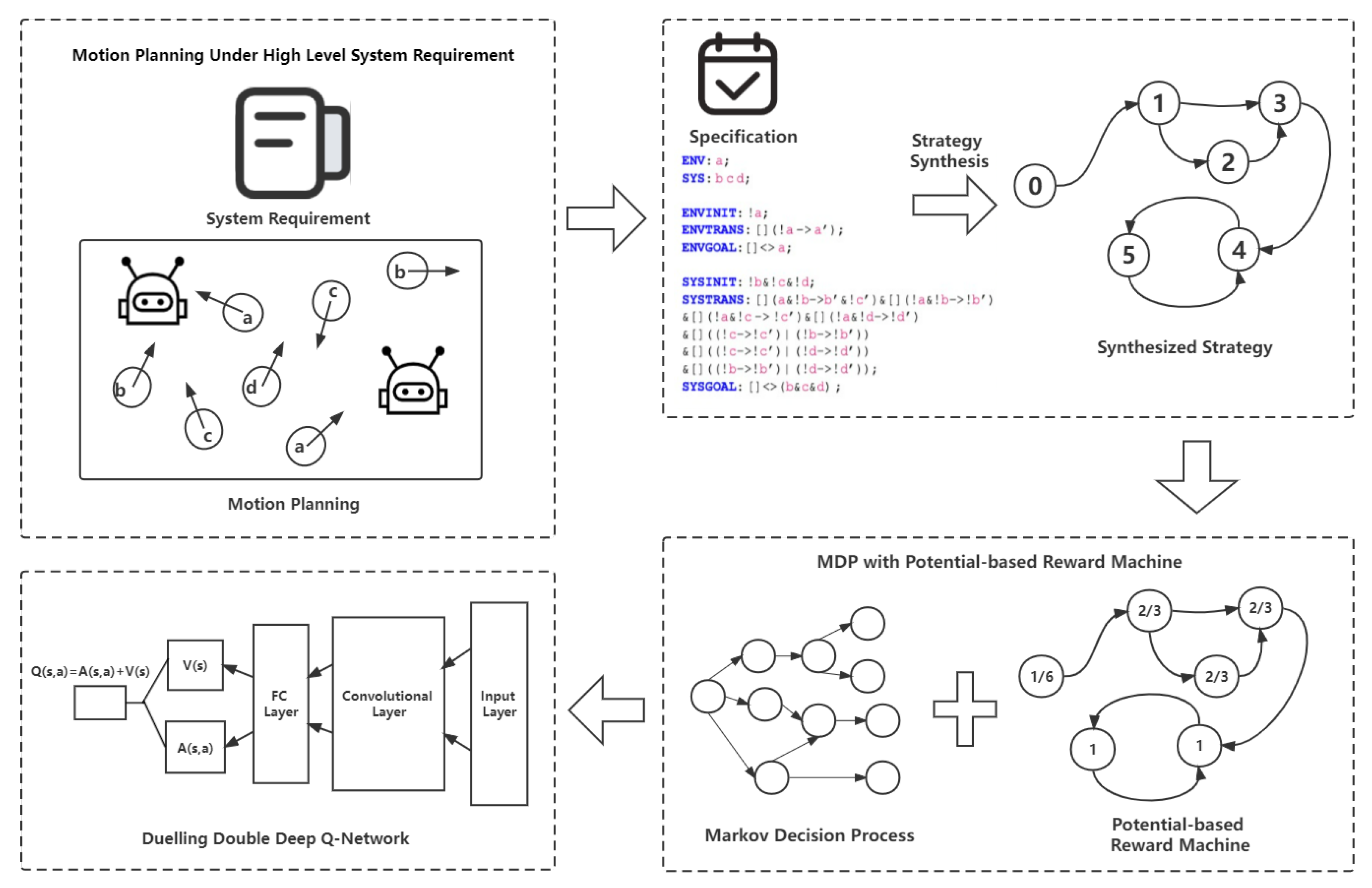
The overall framework is shown in Figure 3. We first construct GR(1) specifications from the high-level system requirements, which are used to synthesize the strategy and construct the Potential-Based Reward Machine (PBRM). The GR(1) synthesis tool gr1c [29] is used to construct the synthesized strategy in Figure 2. The synthesized strategy abstracts the environment states and guides the transitions between abstract states. This helps the agent keep track of the abstract states and follow the synthesized strategy to finish the tasks under the required specifications. We then integrate the PBRM with MDP to construct a new MDP, which is trained with a Dueling Double Deep Q-Network.

4.2. Integrating Deep Reinforcement Learning with the GR(1) Strategy

We first extend the synthesized strategy S to the potential-based reward machine N in Definition 1, which introduces the reward function δ r and potential function ϕ into S . Given the current state e, as well as the atomic proposition δ a [ e ] , δ r [ e ] [ δ a [ e ] ] and ϕ [ e ] are calculated based on the status of e. In the cases that the next state in the reward machine is one of the accepting states, formally presented as δ e [ e ] [ δ a [ e ] ] F , then δ r [ e ] [ δ a [ e ] ] is assigned with a constant reward R , and ϕ [ e ] is also assigned the same constant reward R . Here, the reward of the state transition and the potential function is under the same scalar. The accepting states could be used to indicate that the task specifications have been satisfied. In the cases that the next state does not belong to the accepting states, then δ r [ e ] [ δ a [ e ] ] is assigned with 0 and ϕ [ e ] is assigned with the value within the range ( 0 , R ) , which is shown in Equation (7).
Definition 1
(Potential-based Reward Machine). Given the synthesized strategy
S = E , e 0 , F , δ e , δ a ,
the potential-based reward machine is defined as
N = E , e 0 , F , δ e , δ r , ϕ ,
where E is a finite set of states; e 0 E is the initial state; F E is the set of accepting states; δ e E × 2 P E is the transition function between states; δ r E × 2 P R is the rewards function of the state with the transition function; and ϕ E R is the potential function of the states. S and N satisfy:
E = E , e 0 = e 0 , F = F , δ e = δ e δ r [ e ] [ δ a [ e ] ] = 0 δ e [ e ] [ δ a [ e ] ] F R δ e [ e ] [ δ a [ e ] ] F ϕ [ e ] ( 0 , R ) δ e [ e ] [ δ a [ e ] ] F ϕ [ e ] = R δ e [ e ] [ δ a [ e ] ] F
Then, we extend the MDP with N to reward the agents in Definition 2. M and N share the same set of atomic propositions 2 P . Given that the agent is in the state s , e and performs action a to move from state s to s in the MDP with the labeling function L S × A × S 2 P , if e , L ( s , a , s ) ( δ e ) , then N would move from e to δ e ( e , L ( s , a , s ) ) ; otherwise, the reward machine will stay in the state e. The transition probability distribution of M N is the same as M . In M , R = R when the task specifications are satisfied, and R = 0 otherwise. As shown in Equation (8), the reward function is updated with the potential functions as δ r ( e , L ( s , a , s ) ) + γ ϕ ( e ) ϕ ( e ) if the next state is the accepting state; otherwise, the reward is δ r ( e , L ( s , a , s ) ) . Here, δ r and ϕ are in the same scalar based on Definition 1 to balance the impact of M and N .
Definition 2
(MDP with Potential-based Reward Machine). Given a potential-based reward machine N = E , e 0 , F , δ e , δ a , ϕ and the MDP M = S , s 0 , A , P , R , γ , where M and N share the labeling function L . The MDPPBRM is defined as M N = S ^ , s 0 ^ , A , P ^ , R ^ , γ , where:
S ^ = S × E s 0 ^ = s 0 × e 0 P ^ ( s , e s , e , a ) = P ( s s , a ) R ^ ( s , e , a , s , e ) = δ r ( e , L ( s , a , s ) ) e = e δ r ( e , L ( s , a , s ) ) + γ ϕ ( e ) ϕ ( e ) e e δ r and ϕ are in the same scalar
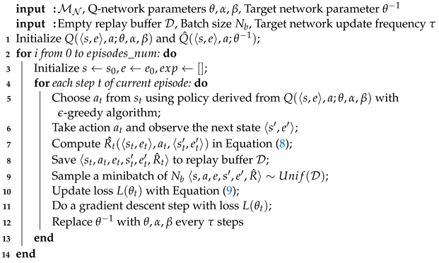
Based on M N , we develop a Dueling Double Deep Q-Network in Algorithm 1 to aid the agents in learning motion planning strategies under GR(1) specifications. Algorithm 1 takes in the extended MDP M N ; the Q-network parameters θ , α , β ; the target network parameter θ 1 ; the empty replay buffer D ; batch size N b ; and target network update frequency τ . For each step t of each episode, Algorithm 1 follows the standard routine of DQN that uses the policy derived from Q ( s , e , a ; θ , α , β ) with the ϵ -greedy approach to select actions a t . The agent then takes action a t and observes the next state s , e . The reward is calculated based on Equation (8). If the next state is the accepting state, then δ r ( e , L ( s , a , s ) ) + γ ϕ ( e ) ϕ ( e ) ; otherwise, the the reward is δ r ( e , L ( s , a , s ) ) . Then, the transition and the reward pair s t , a t , e t , s t , e t , R ^ t are saved to the replay buffer D for sampling. During the training step, a mini-batch of N b is sampled. The loss function L ( θ t ) is calculated based on the mini-batch data in Equation (9). In the case that e is in the accepting state, then the target value is R t ; otherwise, the target value is R t + γ Q ^ ( s t + 1 , a r g m a x Q ( s t + 1 , a ; θ t ) ; θ t 1 ) . Then, the gradient descent optimization is used to set the weight values of θ , α , β . Q-network parameters Q are copied to the target network Q ^ every τ step:
L ( θ t ) = E R t Q s , a ; θ t , α t , β t 2 e T e r m i n a l E R t + γ Q ^ ( s t + 1 , a r g m a x Q ( s t + 1 , a ; θ t ) ; θ t 1 ) Q s , a ; θ t , α t , β t 2 e T e r m i n a l
Algorithm 1: Dueling Double Deep Q-Network on M N synthesized from GR(1) formula.
Electronics 11 03716 i001

4.3. Topological-Sort-Based Reward Shaping

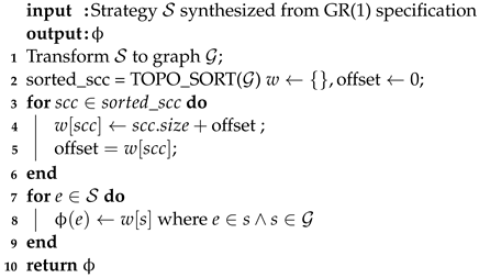
In typical DRL algorithms, the reward would only be assigned when the agent has accomplished the whole task, leading to sparse reward issues. It becomes challenging for the agents to learn the correct actions during intermediate steps. Reward shaping can provide intermediate rewards to the agent so that the agent knows which action to take under the current state. Potential-based Reward Shaping (PBRS) uses the difference in the potential values of different states to guarantee policy invariance [30]. Based on PBRS, work in [3] proposed using value iteration to approximate the cumulative discounted reward in the reward machine. However, the potential values calculated with this approach highly depend on the discount factor γ r . Given that the shortest distance between state s to the terminal state is d, then ϕ ( s ) = γ r d . Given that the initial state s 0 is close to the terminal state, then ϕ ( s 0 ) would be close to the potential value of the terminal state, making the training process less effective. In addition, we observe that the value iteration approach is less practical in the cases of reward machines with Strongly Connected Components (SCC). Based on the reward machine constructed from the synthesized strategy from GR(1) specifications, we develop a topological-sort-based reward-shaping approach in Algorithm 2 to calculate the potential values of reward machines with DCG.
Algorithm 2 takes the synthesized strategy from GR(1) specifications as the input and outputs the potential values of the reward machine states, which can be integrated with the strategy to construct the potential-based reward machine N . We first transform the strategy S to a DCG G . In the transformed graph, the vertices represent the states of S , and the edges represent the transitions of S . We then apply topology sort on the graph G and obtain all the SCCs within the graph. Here, we use s o r t e d _ s c c to denote the set of SCCs. Let t p s o r t e d _ s c c [ 1 , n ] be the topological order of SCC, which is a bijection function from s o r t e d _ s c c to the order of SCC. Here, n denotes the number of SCCs in the graph. Let w s o r t e d _ s c c R be the potential value of SCC and s i z e s o r t e d _ s c c [ 1 , m ] be the number of elements of the specific SCC, where m denotes the number of vertices in the graph. Then, w is calculated based on Clause (10) (line 4–5). All the elements e within the same SCC shares the same potential value w [ s ] (line 8). In summary, Algorithm 2 calculates the SCC in S and assigns the weight of each SCC based on its topological order and the number of elements:
w [ s ] = ( i = 1 i < t p [ s ] s i z e [ t p 1 [ i ] ] ) + s i z e [ s ] , s s o r t e d _ s c c
Algorithm 2: Topological-sort-Based Reward-Shaping Algorithm.
Electronics 11 03716 i002

5. Experimental Section

This section presents empirical evaluations of the proposed algorithms in two experimental settings. We used three GR(1) specifications to specify the reactive multi-task specifications in different stochastic environments, whose synthesized strategies are shown in Figure 4. In this setting, we assumed that two agents were trying to reach the swarm robotics and finish their collecting tasks, one of which was the initiative agent and the other being the passive agent. The initiative agent was specified with the environment assumptions, and the passive agent was specified under the system guarantees in the GR(1) specification. The specifications of the passive agents are required to be satisfied only if the specifications of the initiative agents are satisfied. The algorithms are tests on the initiative agent and passive agent. We assume that each agent has ten sensors pointing in different directions, and each direction observes five variables: the range (x,y direction), the category of the sensed robot and the velocity of the sensed swarm robot (x,y direction). In addition, there are two additional sensors for their value in both the x and y directions. All these values are real numbers. So, the state is a 52-dimensional continuous state space. Moreover, action is a four-dimensional discrete space, which moves in four different directions.

5.1. Experiment Setup

In this section, we compare the GR(1)-guided Dueling Double DQN with Topological-Sort-based Reward Shaping (GR(1)-3DQN-TSRS), GR(1)-guided Double DQN with Topological-Sort-based Reward Shaping (GR(1)-2DQN-TSRS) and GR(1)-guided DQN with Topological-Sort-based Reward Shaping (GR(1)-DQN-TSRS) against three state-of-art baselines algorithms: GR(1)-guided DQN (GR(1)-DQN), GR(1)-guided DQN with Value-Iteration-based Reward Shaping (GR(1)-DQN-VIRS) and Hierarchical RL for Reward Machines (HRL) [3]. The HRL approach decomposes the multiple tasks into options, all of which would be learned simultaneously through off-policy learning. We first implemented Algorithms 1 and 2 under the OpenAI Gym environment [31] with the stochastic environment settings shown in Figure 1a. We compared the learning rate and the optimal reward of these algorithms with two different settings:
  • Different GR(1) specifications under the same environment;
  • Different environments under the same GR(1) specification.
The hyper-parameter settings of the experiment are shown in Table 1. For each experiment, we calculated the learning curve for the average reward per step. In addition, we use the mean value, standard deviation and maximum value to show the performance of different algorithms.

5.2. Performance Evaluation under Different GR(1) Specifications

In the first experiment, we compare the four algorithms, namely, HRM, GR(1)-DQN, GR(1)-DQN-VIRS and GR(1)-DQN-TSRS under three GR(1) specifications, whose synthesized strategies are in different formats. This experiment aims to show that topological-sort-based reward shaping works better in situations where the synthesized strategies are in the form of DCGs. The synthesized strategies of φ 1 , φ 2 and φ 3 are presented in Figure 4. In the experiment settings, the synthesized strategies of φ 1 are in the form of Directed Acyclic Graphs (DAG), and those of φ 2 and φ 3 are in the form of DCGs.
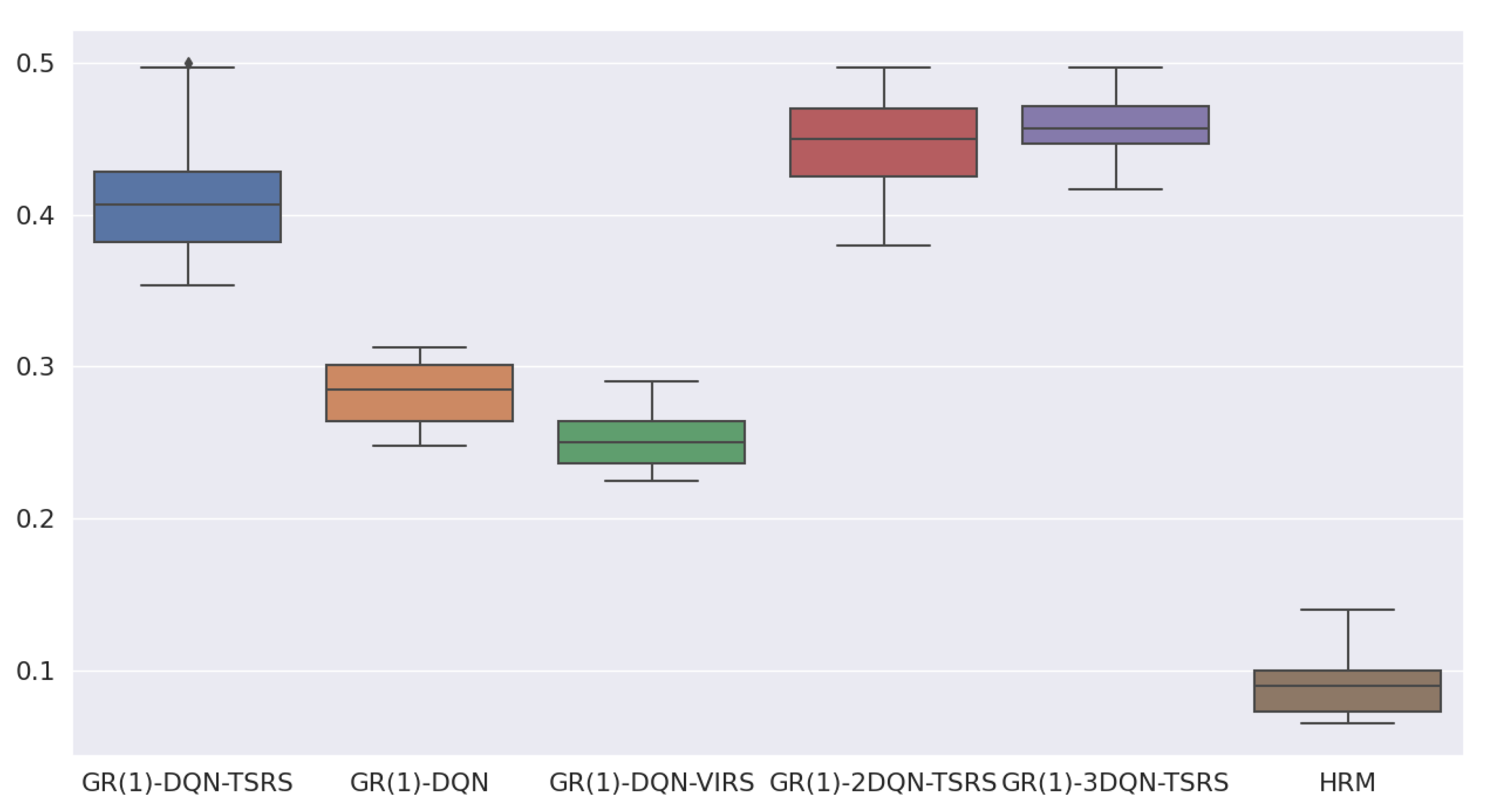
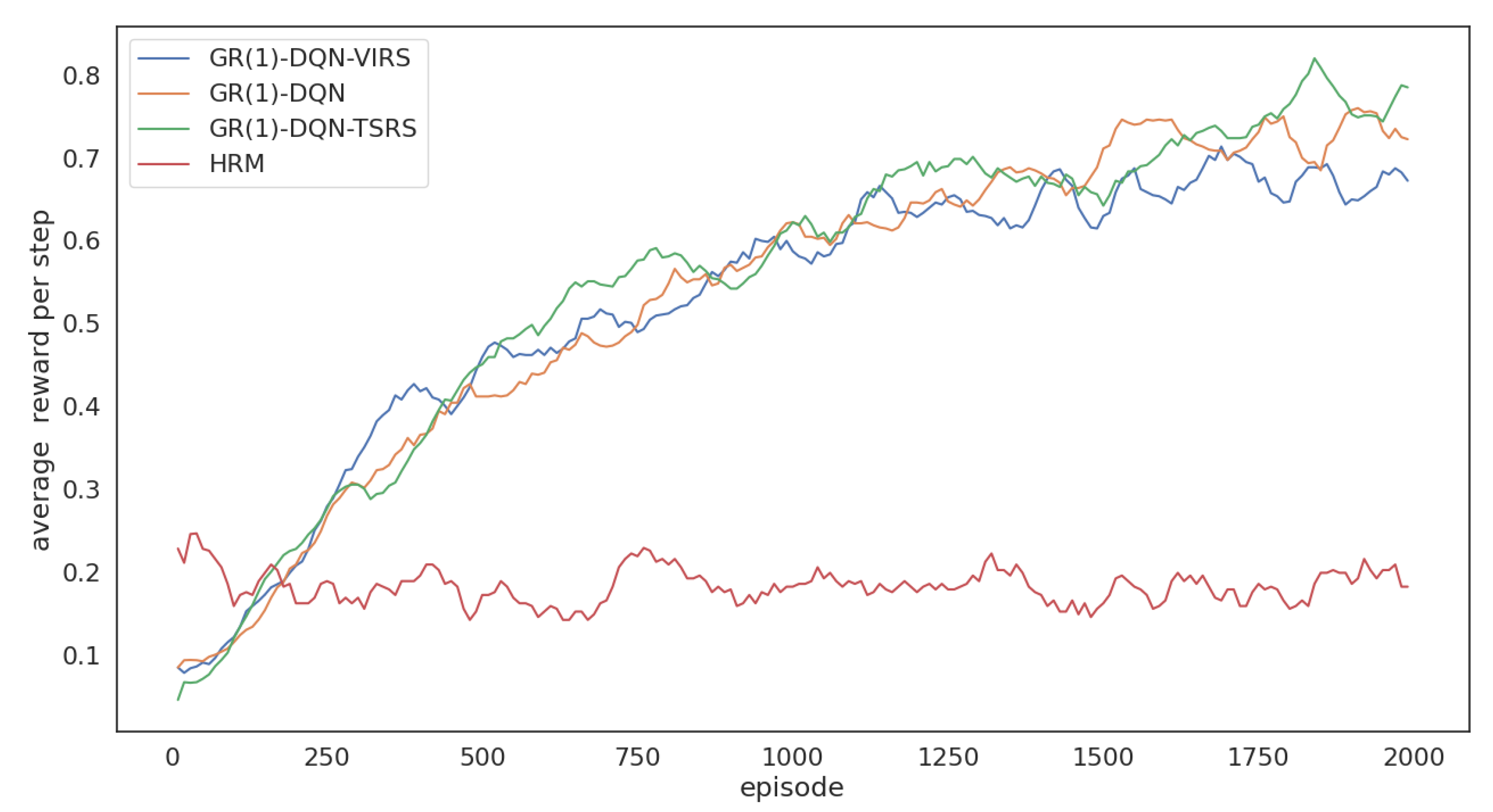
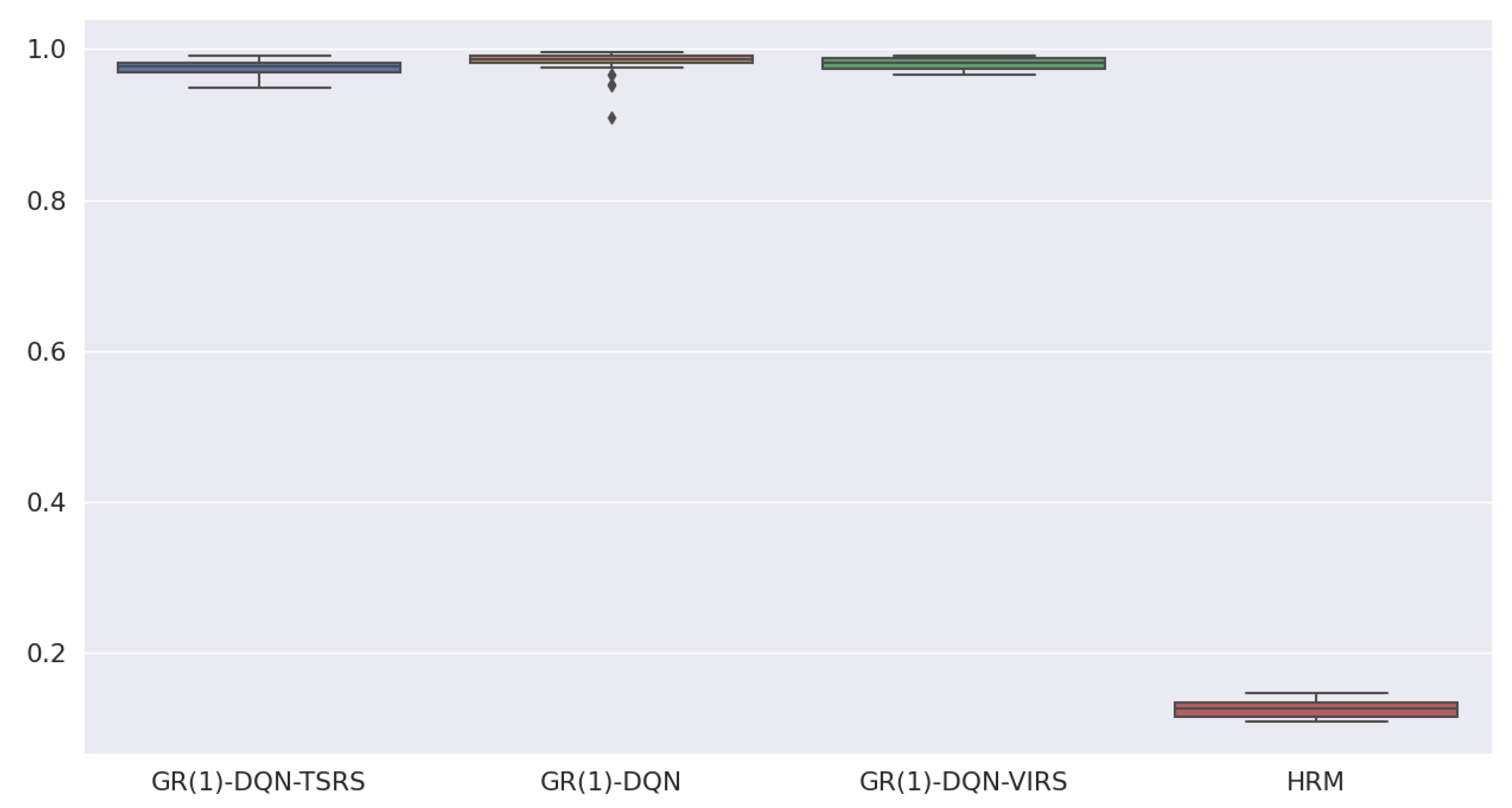
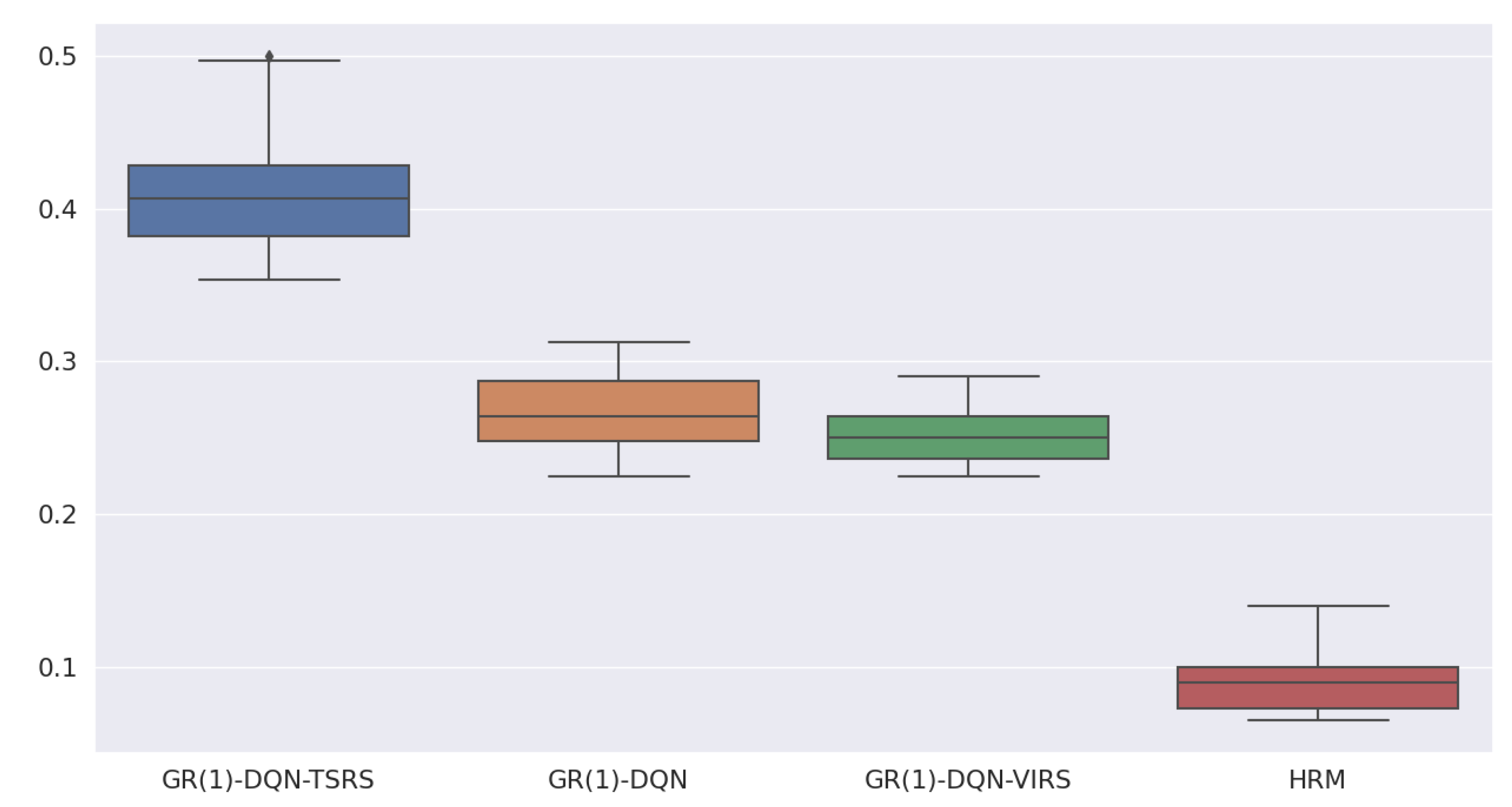
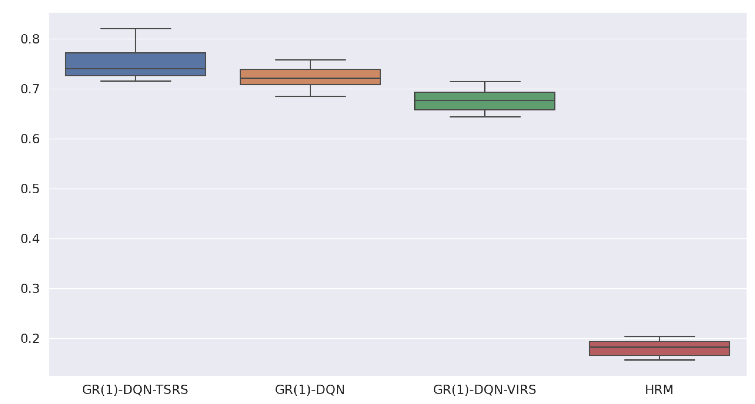
Figure 5, Figure 6 and Figure 7 show the comparison of the learning curves of the algorithms using different GR(1) specifications under the same environment. The results show that the GR(1)-DQN, GR(1)-DQN-VIRS and GR(1)-DQN-TSRS learn faster than HRM under all GR(1) specifications. Figure 8, Figure 9 and Figure 10 show the box plot of the learning curve for different GR(1) specifications. Table 2 shows the mean, maximum and standard deviation of the learning curves of different models. As can be seen from the values, GR(1)-DQN, GR(1)-DQN-VIRS and GR(1)-DQN-TSRS have higher rewards per step compared with HRM in all the three cases. Furthermore, in the cases where the synthesized strategy is in the form of DAGs, GR(1)-DQN, GR(1)-DQN-VIRS and GR(1)-DQN-TSRS have similar mean rewards. For example, GR(1)-DQN obtained 0.982 per step, GR(1)-DQN-VIRS obtained 0.981 per step and GR(1)-DQN-TSRS obtained 0.974 per step. However, in the cases that the synthesized strategy is in the form of DCGs, GR(1)-DQN-TSRS has higher mean rewards and maximum rewards compared with GR(1)-DQN and GR(1)-DQN-VIRS. For example, in the φ 2 and φ 3 specifications, the GR(1)-DQN-TSRS model obtained the highest mean and maximum reward in both cases. So, the experiment results concluded that the GR(1)-DQN-TSRS approach could obtain a higher accumulated reward compared with HRM, GR(1)-DQN and GR(1)-DQN-VIRS.

5.3. Ablation Study under Different Environment Settings

We use φ 2 as the GR(1) specification in the second experiment and perform an ablation study with three different stochastic environments. Different stochastic environment settings will also have an impact on the learning efficiency of agents, for example, if the task specification requires the agent to reach swarm agent b after reaching swarm agent a, where a and b are close on the map. In this case, it would be easy for the agents to learn the policy to move from a to b. However, if a and b are far from each other in another stochastic map, then it would be inefficient for the agents to learn the policy for motion planning under complicated task specifications.
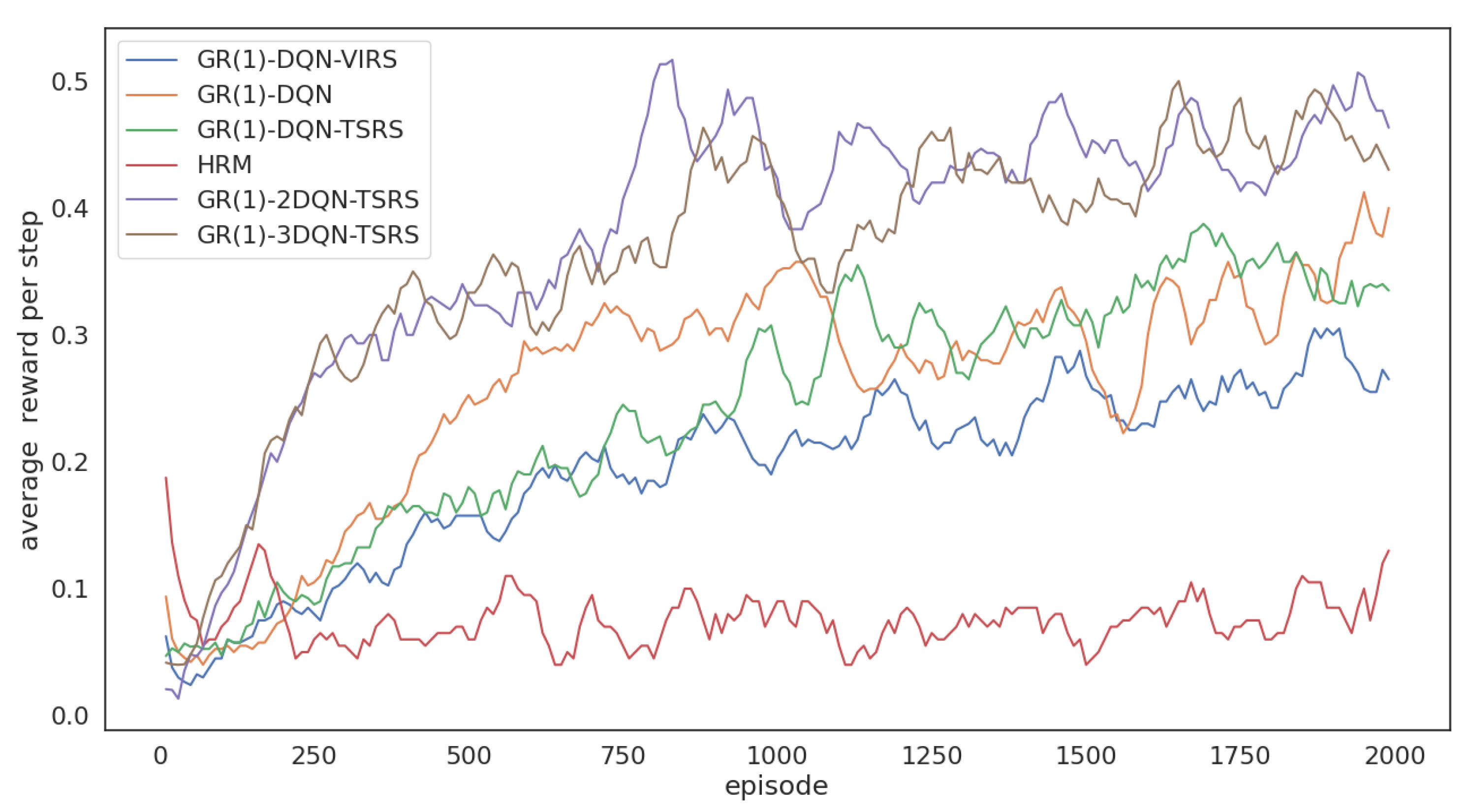
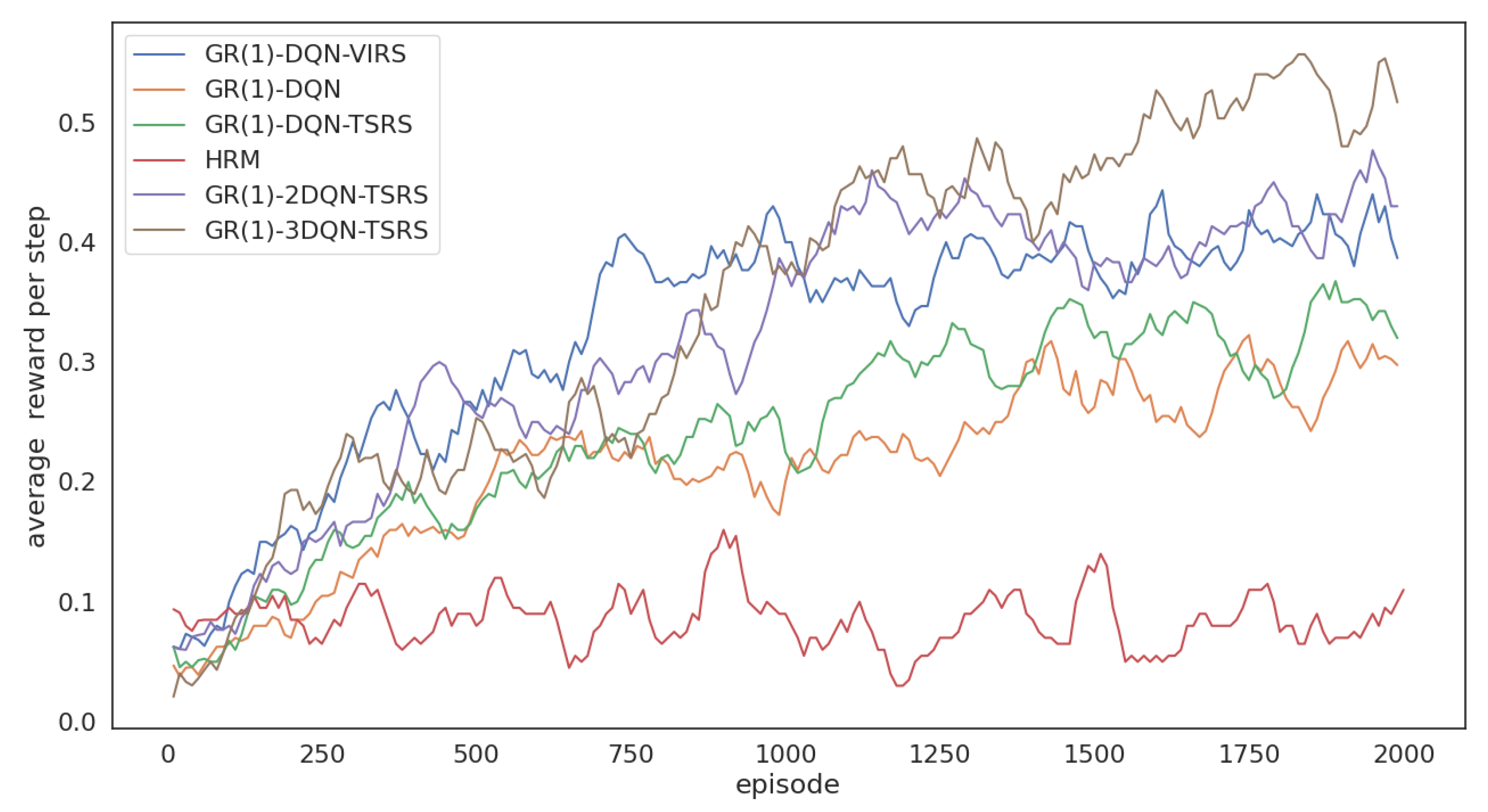
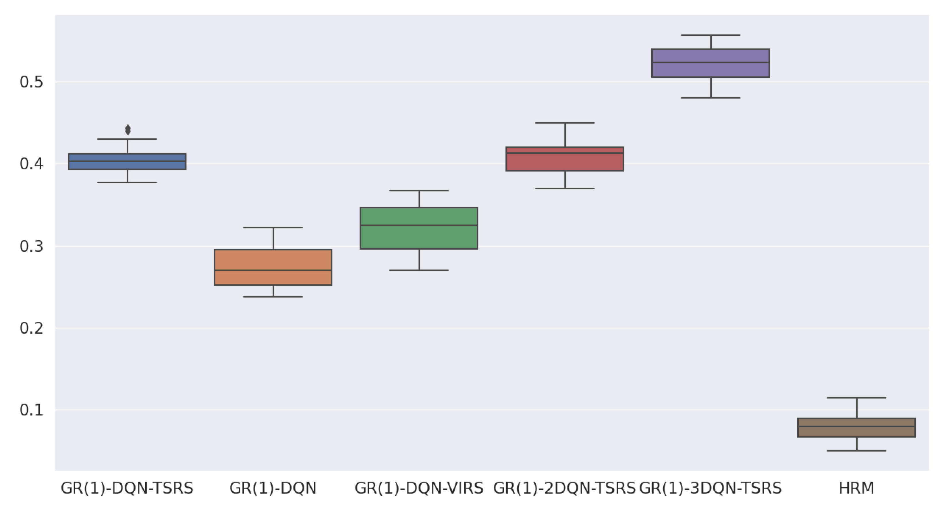
In this ablation study, we mainly examine the performances of six algorithms in three different environments, namely, HRM, GR(1)-DQN, GR(1)-DQN-VIRS, GR(1)-DQN-TSRS, GR(1)-2DQN-TSRS and GR(1)-3DQN-TSRS. Figure 11, Figure 12 and Figure 13 show the learning curve of these six algorithms under different environment settings. Figure 14, Figure 15 and Figure 16 show the box plot of different algorithms in three environments. Table 3 shows the mean, maximum and standard deviation of the learning curves of different models under different maps. Firstly, we observe that the GR(1)-DQN-TSRS, GR(1)-2DQN-TSRS and GR(1)-3DQN-TSRS performs better than HRM, GR(1)-DQN and GR(1)-DQN-VIRS in the three maps. GR(1)-3DQN-TSRS obtained the highest mean and maximum value in M2 and M3. GR(1)-DQN-TSRS obtained the maximum reward in M1. All the approaches have similar variances. From the learning curve and the table, we could observe the following conclusions:
  • HRM obtains the lowest reward compared with the other five algorithms;
  • GR(1)-DQN and GR(1)-DQN-VIRS have similar performances, but their reward per step is smaller than the topological-sort-based reward-shaping approaches;
  • It is evident that topological-sort-based reward shaping could help GR(1)-DQN obtain more rewards during training;
  • Overall GR(1)-2DQN-TSRS is better than GR(1)-DQN-TSRS, and GR(1)-3DQN-TSRS is better than GR(1)-2DQN-TSRS.
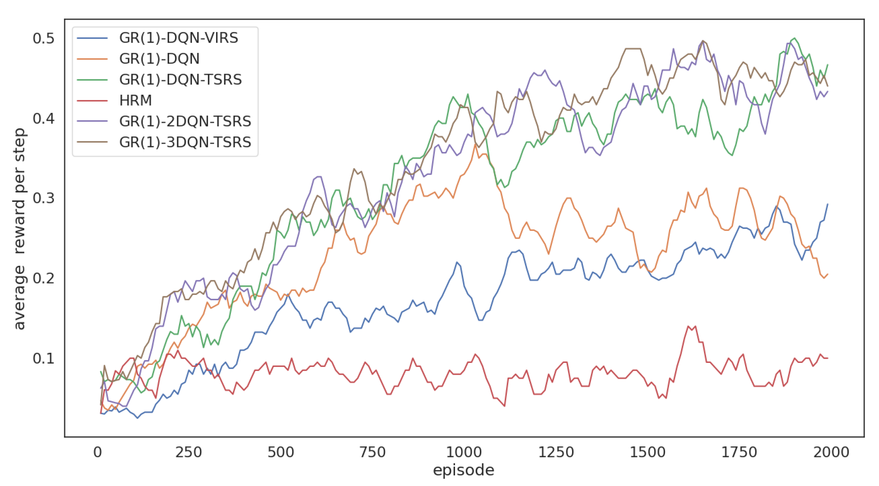
Figure 11. Comparison of learning curves for multi-task reinforcement learning algorithms with φ 2 under stochastic environment setting 1.
Electronics 11 03716 g011
Figure 12. Comparison of learning curves for multi-task reinforcement learning algorithms with φ 2 under stochastic environment setting 2.
Electronics 11 03716 g012
Figure 13. Comparison of learning curves for multi-task reinforcement learning algorithms with φ 2 under stochastic environment setting 3.
Electronics 11 03716 g013
Figure 14. Box plot of learning curve for φ 2 under the environment setting 1.
Electronics 11 03716 g014
Figure 15. Box plot of learning curve for φ 2 under the environment setting 2.
Electronics 11 03716 g015
Figure 16. Box plot of learning curve for φ 2 under the environment setting 3.
Electronics 11 03716 g016

6. Conclusions

This paper considers one fragment of LTL, GR(1), as a high-level reactive temporal logic to guide robots in learning efficient movement strategies under stochastic environments. The GR(1) specifications used in this paper, whose control policy can be synthesized in polynomial time, are applicable in industrial applications. Taking the synthesized strategies of GR(1) specifications as the potential-based reward machine, we extend MDP with a topological-sort-based reward-shaping approach to improve learning efficiency. The reward machine is then integrated with the dueling double deep network to guide motion planning under continuous state space. Experiments on multi-task learning under GR(1) specifications show that the proposed approach outperforms the state-of-art algorithms in learning efficiency and optimal rewards per step. In addition, compared with the value-iteration-based reward-shaping approaches, our topological-sort-based reward-shaping approach could handle the cases where the synthesized strategies are in the form of DCGs.
There still exist some research challenges for future work. For example, the initial GR(1) specification could be incomplete and unrealizable. We could develop a counter-strategy-based framework to refine the GR(1) specifications with realizable strategies. In addition, this paper mainly focuses on value-based DRL approaches. In future work, we might explore the possibilities of integrating GR(1) specifications with policy-based approaches such as PPO.

Author Contributions

Conceptualization, C.Z. and Y.C.; methodology, C.Z.; software, C.Z.; validation, C.Z., J.Z. and C.H.; formal analysis, J.B.; investigation, C.Z.; resources, C.Z.; data curation, C.Z.; writing—original draft preparation, C.Z.; writing—review and editing, J.B.; visualization, J.Z.; supervision, C.Z.; project administration, C.Z.; funding acquisition, C.Z. All authors have read and agreed to the published version of the manuscript.

Funding

This work was supported by the Natural Science Foundation of the Higher Education Institutions of Jiangsu Province (No. 22KJB520012) and the Postgraduate Research and Practice Innovation Project of Jiangsu Province (No. KYCX223060).

Institutional Review Board Statement

Not applicable.

Informed Consent Statement

Not applicable.

Data Availability Statement

Not applicable.

Conflicts of Interest

The authors declare no conflict of interest.

Abbreviations

The following abbreviations are used in this manuscript:
DRLDeep Reinforcement Learning
LTLLinear Temporal Logic
GR(1)Generalized Reactivity of rank 1
DCGDirected Cyclic Graphs
DAGDirected Acyclic Graphs
3DQNDueling Double Deep Q-Network
2DQNDouble Deep Q-Network
DQNDeep Q-Network
RLReinforcement Learning
PBRMPotential-Based Reward Machine
PBRSPotential-based Reward Shaping
SCCStrongly Connected Components
LDBALimit-Deterministic Büchi Automata
DFADeterministic Finite Automata

References

  1. Kulkarni, T.D.; Narasimhan, K.; Saeedi, A.; Tenenbaum, J. Hierarchical deep reinforcement learning: Integrating temporal abstraction and intrinsic motivation. Adv. Neural Inf. Process. Syst. 2016, 29, 1–11. [Google Scholar]
  2. Toro Icarte, R.; Klassen, T.Q.; Valenzano, R.; McIlraith, S.A. Teaching multiple tasks to an RL agent using LTL. In Proceedings of the 17th International Conference on Autonomous Agents and MultiAgent Systems(AAMAS), Stockholm, Sweden, 10–15 July 2018; pp. 452–461. [Google Scholar]
  3. Icarte, R.T.; Klassen, T.Q.; Valenzano, R.; McIlraith, S.A. Reward machines: Exploiting reward function structure in reinforcement learning. J. Artif. Intell. Res. 2022, 73, 173–208. [Google Scholar] [CrossRef]
  4. Pnueli, A.; Rosner, R. On the synthesis of a reactive module. In Proceedings of the 16th ACM SIGPLAN-SIGACT Symposium on Principles of Programming Languages, Austin, TX, USA, 11–13 January 1989; pp. 179–190. [Google Scholar]
  5. Kress-Gazit, H.; Fainekos, G.E.; Pappas, G.J. Temporal-logic-based reactive mission and motion planning. IEEE Trans. Robot. 2009, 25, 1370–1381. [Google Scholar] [CrossRef] [Green Version]
  6. Li, R.; Shi, H.; Liu, W.; Dong, W. Synthesizing Cooperative Controllers from Global Tasks of Multi-robot Systems. In Proceedings of the 2020 IEEE 27th Asia-Pacific Software Engineering Conference (APSEC), Singapore, 1–4 December 2020; pp. 109–118. [Google Scholar]
  7. Wang, C.; Li, Y.; Smith, S.L.; Liu, J. Continuous motion planning with temporal logic specifications using deep neural networks. arXiv 2020, arXiv:2004.02610. [Google Scholar]
  8. Li, X.; Serlin, Z.; Yang, G.; Belta, C. A formal methods approach to interpretable reinforcement learning for robotic planning. Sci. Robot. 2019, 4, eaay6276. [Google Scholar] [CrossRef] [PubMed]
  9. Fu, J.; Topcu, U. Probably approximately correct MDP learning and control with temporal logic constraints. arXiv 2014, arXiv:1404.7073. [Google Scholar]
  10. Jothimurugan, K.; Bansal, S.; Bastani, O.; Alur, R. Compositional reinforcement learning from logical specifications. Adv. Neural Inf. Process. Syst. 2021, 34, 10026–10039. [Google Scholar]
  11. Li, X.; Vasile, C.I.; Belta, C. Reinforcement learning with temporal logic rewards. In Proceedings of the IEEE 2017 IEEE/RSJ International Conference on Intelligent Robots and Systems (IROS), Vancouver, BC, Canada, 24–28 September 2017; pp. 3834–3839. [Google Scholar]
  12. Bozkurt, A.K.; Wang, Y.; Zavlanos, M.M.; Pajic, M. Model-free reinforcement learning for stochastic games with linear temporal logic objectives. In Proceedings of the IEEE 2021 IEEE International Conference on Robotics and Automation (ICRA), Xi’an, China, 30 May–5 June 2021; pp. 10649–10655. [Google Scholar]
  13. Kantaros, Y.; Zavlanos, M.M. Stylus*: A temporal logic optimal control synthesis algorithm for large-scale multi-robot systems. Int. J. Robot. Res. 2020, 39, 812–836. [Google Scholar] [CrossRef]
  14. De Giacomo, G.; Iocchi, L.; Favorito, M.; Patrizi, F. Foundations for restraining bolts: Reinforcement learning with LTLf/LDLf restraining specifications. In Proceedings of the International Conference on Automated Planning and Scheduling(ICAPS), Berkeley, CA, USA, 10–15 July 2019; Volume 29, pp. 128–136. [Google Scholar]
  15. Wen, M. Reinforcement Learning With High-Level Task Specifications. Ph.D. Thesis, University of Pennsylvania, Philadelphia, PA, USA, 2019. [Google Scholar]
  16. Bozkurt, A.K.; Wang, Y.; Zavlanos, M.M.; Pajic, M. Control synthesis from linear temporal logic specifications using model-free reinforcement learning. In Proceedings of the 2020 IEEE International Conference on Robotics and Automation (ICRA), Paris, France, 31 May–31 August 2020; pp. 10349–10355. [Google Scholar]
  17. Hasanbeig, M.; Abate, A.; Kroening, D. Certified reinforcement learning with logic guidance. arXiv 2019, arXiv:1902.00778. [Google Scholar]
  18. Icarte, R.T.; Klassen, T.; Valenzano, R.; McIlraith, S. Using reward machines for high-level task specification and decomposition in reinforcement learning. In Proceedings of the International Conference on Machine Learning (ICML), PMLR, Stockholm, Sweden, 10–15 July 2018; pp. 2107–2116. [Google Scholar]
  19. Camacho, A.; Toro Icarte, R.; Klassen, T.Q.; Valenzano, R.; McIlraith, S.A. LTL and Beyond: Formal Languages for Reward Function Specification in Reinforcement Learning. In Proceedings of the Twenty-Eighth International Joint Conference on Artificial Intelligence (IJCAI), Macao, China, 10–16 August 2019; pp. 6065–6073. [Google Scholar]
  20. Pnueli, A. The temporal logic of programs. In Proceedings of the IEEE 18th Annual Symposium on Foundations of Computer Science (sfcs 1977), Providence, RI, USA, 31 October–2 November 1977; pp. 46–57. [Google Scholar] [CrossRef]
  21. Piterman, N.; Pnueli, A.; Sa’ar, Y. Synthesis of reactive (1) designs. In Proceedings of the International Workshop on Verification, Model Checking, and Abstract Interpretation; Springer: Berlin/Heidelberg, Germany, 2006; pp. 364–380. [Google Scholar]
  22. Kaelbling, L.P.; Littman, M.L.; Moore, A.W. Reinforcement learning: A survey. J. Artif. Intell. Res. 1996, 4, 237–285. [Google Scholar] [CrossRef] [Green Version]
  23. Watkins, C.J.; Dayan, P. Q-learning. Mach. Learn. 1992, 8, 279–292. [Google Scholar] [CrossRef]
  24. Mnih, V.; Kavukcuoglu, K.; Silver, D.; Graves, A.; Antonoglou, I.; Wierstra, D.; Riedmiller, M. Playing atari with deep reinforcement learning. arXiv 2013, arXiv:1312.5602. [Google Scholar]
  25. Thrun, S.; Schwartz, A. Issues in using function approximation for reinforcement learning. In Proceedings of the 1993 Connectionist Models Summer School; Lawrence Erlbaum: Hillsdale, NJ, USA, 1993; Volume 6, pp. 1–9. [Google Scholar]
  26. Van Hasselt, H.; Guez, A.; Silver, D. Deep reinforcement learning with double q-learning. In Proceedings of the AAAI conference on Artificial Intelligence, Phoenix, AZ, USA, 12–17 February 2016; Volume 30. [Google Scholar]
  27. Wang, Z.; Schaul, T.; Hessel, M.; Hasselt, H.; Lanctot, M.; Freitas, N. Dueling network architectures for deep reinforcement learning. In Proceedings of the International Conference on Machine Learning, PMLR, New York, NY, USA, 20–22 June 2016; pp. 1995–2003. [Google Scholar]
  28. Hu, Y.; Wang, W.; Jia, H.; Wang, Y.; Chen, Y.; Hao, J.; Wu, F.; Fan, C. Learning to utilize shaping rewards: A new approach of reward shaping. Adv. Neural Inf. Process. Syst. 2020, 33, 15931–15941. [Google Scholar]
  29. Livingston, S. GR1C: A collection of Tools for GR(1) Synthesis and Related Activities. Github. Available online: https://scottman.net/2012/gr1c (accessed on 26 October 2022).
  30. Ng, A.Y.; Harada, D.; Russell, S. Policy invariance under reward transformations: Theory and application to reward shaping. In Proceedings of the Sixteenth International Conference on Machine Learning, Bled, Slovenia, 27–30 June 1999; Volume 99, pp. 278–287. [Google Scholar]
  31. Brockman, G.; Cheung, V.; Pettersson, L.; Schneider, J.; Schulman, J.; Tang, J.; Zaremba, W. Openai gym. arXiv 2016, arXiv:1606.01540. [Google Scholar]
Figure 1. Example showing motion planning under a stochastic environment. (a) Motion planning under stochastic environment. (b) Synthesized strategy of the example.
Electronics 11 03716 g001
Figure 3. Overall Framework that Guides Deep Reinforcement Learning with High-level GR(1) Specifications.
Electronics 11 03716 g003
Figure 4. The synthesized strategies used in the experiment.
Electronics 11 03716 g004
Figure 5. Comparison of learning curves for multi-task reinforcement learning algorithms with φ 1 under the same stochastic environment.
Electronics 11 03716 g005
Figure 6. Comparison of learning curves for multi-task reinforcement learning algorithms with φ 2 under the same stochastic environment.
Electronics 11 03716 g006
Figure 7. Comparison of learning curves for multi-task reinforcement learning algorithms with φ 3 under the same stochastic environment.
Electronics 11 03716 g007
Figure 8. Box plot of learning curve for φ 1 under the same environment.
Electronics 11 03716 g008
Figure 9. Box plot of learning curve for φ 2 under the same environment.
Electronics 11 03716 g009
Figure 10. Box plot of learning curve for φ 3 under the same environment.
Electronics 11 03716 g010
Table 1. The Hyper-parameter Settings of the Experiments.
Hyper-ParameterDefinitionValue
D _ s i z e replay buffer size50,000
l a y e r _ n u m number of layers4
a c t i v a t i o n activation functionRelu
N b batch size32
τ target network update frequency100
s t e p s _ p e r _ e p i s o d e number of steps per episode1000
t o t a l _ e p i s o d e total number of episodes2000
Table 2. The mean, max and standard deviation of learning curves from specification φ 1 , φ 2 and φ 3 starting from training step 1600.
HRMGR(1)-DQNGR(1)-DQN-VIRSGR(1)-DQN-TSRS
mean0.1260.9820.9810.974
φ 1 std0.00010.00030.00010.0001
max0.1480.9960.9910.991
mean0.0920.2840.2510.411
φ 2 std0.00050.00040.00030.0017
max0.1400.3130.2900.500
mean0.1810.7220.6760.752
φ 3 std0.00020.00040.00040.0009
max0.2030.7560.7140.820
Table 3. The mean, max and standard deviation of learning curves from maps M1, M2 and M3 starting from training step 1600.
HRMGR(1)
-DQN
GR(1)
-DQN
-VIRS
GR(1)
-DQN
-TSRS
GR(1)
-2DQN
-TSRS
GR(1)
-3DQN
-TSRS
mean0.0910.2480.2510.4110.4500.458
M1std0.00050.00040.00030.00170.00100.0004
max0.1400.3130.2900.5000.4970.497
mean0.0820.3280.2610.3580.4450.461
M2std0.00020.00040.00040.00020.00060.0005
max0.1100.3650.3050.3880.4970.500
mean0.0800.2700.3200.4040.4080.522
M3std0.00020.00060.00080.00030.00040.0004
max0.1150.3230.3680.4430.4500.557
Publisher’s Note: MDPI stays neutral with regard to jurisdictional claims in published maps and institutional affiliations.