Hyperspectral Image Classification Based on Transposed Convolutional Neural Network Transformer

Abstract

Hyperspectral imaging is a technique that captures images of objects within a wide spectrum range, allowing for the acquisition of additional spectral information to reveal subtle variations and compositional components in the objects. Convolutional neural networks (CNNs) have shown remarkable feature extraction capabilities for HSI classification, but their ability to capture deep semantic features is limited. On the other hand, transformer models based on attention mechanisms excel at handling sequential data and have demonstrated great potential in various applications. Motivated by these two facts, this paper proposes a multiscale spectral–spatial transposed transformer (MSSTT) that captures the high-level semantic features of an HSI while preserving the spectral information as much as possible. The MSSTT consists of a spectral–spatial Inception module that extracts spectral and spatial features using multiscale convolutional kernels, and a spatial transpose Inception module that further enhances and extracts spatial information. A transformer model with a cosine attention mechanism is also included to extract deep semantic features, with the QKV matrix constrained to ensure the output remains within the activation range. Finally, the classification results are obtained by applying a linear layer to the learnable tokens. The experimental results from three public datasets show that the proposed MSSTT outperforms other deep learning methods in HSI classification. On the India Pines, Pavia University, and Salinas datasets, accuracies of 97.19%, 99.47%, and 99.90% were achieved, respectively, with a training set proportion of 5%.

1. Introduction

In recent years, there have been significant advancements in remote sensing software and hardware technology [1,2,3,4,5], leading to its increasing applicability in various industries. Among the different remote sensing techniques, hyperspectral imaging [6] has gained considerable attention. By combining spatial features with high-resolution spectral data from different objects, it enables the detection of subtle features in ground object spectra. This fine spectral resolution provides abundant information for applications in diverse fields, such as geology, medical diagnosis, vegetation survey, agriculture [7], environment, military, aerospace, and others.

To effectively utilize the rich information contained in hyperspectral images, a range of techniques have been investigated for hyperspectral data processing, such as decomposition, monitoring, clustering, and classification [8]. Initially, supervised methods were prevalent in this research domain. For instance, Farid et al. [9] introduced a hyperspectral image classification method using support vector machines (SVMs) in 2004. However, an SVM is less adept at handling high-dimensional data and encounters difficulties when applied to large-scale training samples. As a result, researchers directed their efforts toward improving spectral sensors based on SVMs [10].

Yuliya et al. [11] proposed a novel method for the precise spectral–spatial classification of hyperspectral images at the pixel level. This approach improves classification accuracy by taking into account both spectral and spatial information.

In recent years, the field of image processing has undergone a revolutionary change with the advent of deep learning technologies, particularly the introduction of deep convolutional neural networks (CNNs). This progress has had a significant impact on remote sensing image processing technology, ushering in a new era of deep CNN-based classification techniques. Xiaorui Ma et al. [12] proposed an improved network, called the spatial update depth automatic encoder (SDAE), for extracting and utilizing deep features from hyperspectral images. While this method can generate high-quality spatial and spectral features without requiring manual code definitions, it lacks automation in its network parameters.

Subsequently, deep convolutional neural network (CNN) models [13] have been developed for hyperspectral image classification, utilizing multiple convolutional and pooling layers to extract nonlinear, discriminative, and invariant deep features from HSIs [14]. In addition to deep CNN models, other deep learning architectures, such as recursive neural networks [15,16], deep belief networks [17], generative adversarial networks [18,19], and capsule networks [20], have demonstrated promising results in hyperspectral image classification.

The CNN, with its non-contact and high-precision processing capabilities, has become widely utilized in image processing due to its ability to eliminate the need for manual image preprocessing and complex feature extraction operations. In hyperspectral image (HSI) processing, there are three main methods: the CNN spatial extractor, CNN spectral extractor, and CNN spectral–spatial extractor. Hu et al. [21] proposed an architecture for classifying the spectral domain of hyperspectral images, consisting of an input layer, a convolution layer, a maximum pooling layer, a fully connected layer, and an output layer. Because hyperspectral data are typically 3D, 3D CNNs are employed to extract both the spectral and spatial features from these images. Li et al. [22] presented a 3D CNN framework for accurate HSI classification, effectively extracting combined spectral and spatial features without the need for pre- or postprocessing steps. Roy S. K. et al. [23] introduced a mixed-spectrum CNN approach for HSI classification, employing a 3D CNN to extract spatial–spectral features from spectral bands and then using a 2D CNN to capture more abstract spatial information.

HSI data are characterized by a combination of 2D spatial and 1D spectral information, which is distinct from 3D target images. To address this difference, He et al. [24] proposed a multiscale 3D deep convolutional neural network that can simultaneously learn 2D multiscale spatial features and 1D spectral features from HSI data in an end-to-end fashion. The effectiveness of this method has been demonstrated through its good classification results on publicly available HSI datasets.

A CNN [25] possesses powerful feature extraction capabilities and can be seen as a type of multilayer perceptron (MLP) [26]. It takes advantage of local connections and weight sharing to reduce the number of parameters and overall model complexity. When applied to image data, its benefits become even more prominent. A CNN is able to autonomously extract two-dimensional image features, including the color, texture, shape, and image topology, making it widely used for extracting informative features from images. There are numerous well-established frameworks available for a CNN, each tailored to different tasks. Selecting an appropriate framework for classification tasks is of utmost importance. Furthermore, a CNN predominantly performs feature extraction through convolutional kernel operations, and the size of the convolutional kernel also affects the network’s ability to effectively extract features.

Despite the impressive performance of the CNN model in HSI classification, it is not without limitations. First and foremost, the model may overlook important input information, and the 3D features it extracts tend to mix both spatial and spectral information. While 2D feature extraction mainly captures abstract spatial information, it may not be able to effectively process spectral information. A CNN is a vector-based method that treats inputs as a set of pixel vectors [27]. In the case of HSIs, which consists of hundreds of spectral bands forming two-dimensional images of ground objects, it possesses a sequential data structure. Therefore, a CNN may encounter difficulties in processing hyperspectral pixel vectors, resulting in information loss [28]. In addition, HSIs typically comprise hundreds of bands, making it challenging for the CNN model to capture the sequential correlation between distant bands.

By employing STN [29] to obtain the optimal inputs for CNN-based HSI classification, DropBlock is introduced as a regularization technique for the precise classification of HSIs. An expandable subspace clustering method [30] integrates the learning of concise dictionaries and robust subspace representation, while introducing adaptive spatial regularization to enhance model robustness. Additionally, an efficient solver based on an alternating direction method of multipliers (ADMM) is presented to alleviate the computational complexity of the resulting optimization problem. Experimental results demonstrate that this method exhibits good performance and effectiveness in high-dimensional spectral image clustering. Weisheng Dong [31] achieved denoising of hyperspectral images by modifying the 3D U-net to encode rich multiscale information. Moreover, by decomposing the 3D filtering into 2D spatial filtering and 1D spectral filtering, a significant reduction in the number of network parameters is achieved, thereby lowering the computational complexity.

The year 2017 witnessed the introduction of the Transformer network to the field of natural language processing. This model revolutionized the field by relying solely on the attention mechanism [32], which effectively captures global dependencies from input sequences. In 2021, the ViT model [33] was proposed, marking the first successful application of the transformer architecture in computer vision tasks. However, a significant challenge in this context is the conversion of image pixels into sequence data while mitigating issues of excessive complexity, computational load, and high dimensionality.

In 2021, He et al. introduced an improved transformer model called Dense-Transformer, which incorporates dense connections to capture spectral relationships in sequences and utilizes a multilayer perceptron for classification tasks [34]. The Dense-Transformer addresses the issue of vanishing gradients commonly encountered during the training of traditional transformer networks.

Le et al. proposed the spectral–spatial feature tokenization converter (SSFTT) method, which focuses on capturing spectral–spatial features and high-level semantic features [35]. They constructed a spectral–spatial feature extraction module to obtain low-level features and introduced a Gaussian-weighted feature marker for feature transformation. The transformed features were then fed into the converter encoder module for learning and representation. However, the SSFTT’s spectral–spatial classifier relies on 2D and 3D convolutional kernels for feature extraction. Given that hyperspectral data encompass both spectral and spatial information, using a single convolutional kernel for extracting features can result in the loss of spectral dimension feature information.

Therefore, in this paper, we propose a novel hyperspectral classification framework called transposed CNN-transformer feature extraction. This framework combines multiscale convolution and feature labeling techniques. Additionally, we introduce a cross-sinusoidal attention mechanism and a transposed convolution pair to facilitate the rapid and accurate propagation of the feature information within the network. By integrating these components with a multiscale CNN and feature labeling, we achieve an improved classification performance even when faced with limited training samples.

In order to further extract deep spectral–spatial information and reduce the loss of important spectral–spatial features, as well as achieve higher classification accuracy on small training datasets, this paper makes the following main contributions:

(1) In this paper, we propose the spectral Inception module for extracting hyperspectral imaging spectral sequences. This module employs multiscale 3D convolution kernels to preserve the spectral–spatial information of different feature scales. By performing dimensionality reduction and data enhancement, our approach effectively captures both local and global spectral features.

(2) We propose a spatial transposed Inception module to extract HSI spatial information by utilizing multiscale 2D convolution kernels and connecting the output of the transposed convolutional layer with the initial input to enhance the feature information and facilitate the transmission and reconstruction of spectral–spatial information within the network.

(3) We propose a multi-head cross-sinusoidal threshold attention mechanism that combines convolution kernel spectra and spatial patch tokens, using sine functions to limit the dot product size of Q, K, and V. This ensures that the attention output values fall within the effective range of the activation function due to the periodicity of sine.

2. Multiscale Transposed CNN-Transformer Feature Extraction

The MSSTT framework, proposed in this paper, is depicted in Figure 1 below. It consists of three modules: spectral–spatial information enhancement and extraction using Inception, spatial information enhancement and transmission through transposed Inception, and location-coded feature labeling and cross-sinusoidal limit attention for transformer feature classification.

The first step in our approach involves information extraction. Initially, we employ the 3D Inception module to extract the spectral–spatial information, followed by the utilization of the transposed 2D Inception module to extract the spatial information. The second step focuses on feature position coding. The flattened feature information is marked using standard normal functions. The position information is then marked twice using sine and cosine pairs. These marked sequences are subsequently input into the transformer for feature extraction. In the third step, an improved attention mechanism is employed to determine the relationship between the sequence and spatial features. This enhanced attention mechanism helps capture significant feature dependencies within the data. Finally, we obtain the classification results based on the spatial–spectral characteristics obtained from the previous steps.

2.1. Inception-Based Spectral–Spatial Information Enhancement Extraction

The original hyperspectral data are represented by $X\in R^{m\times n\times s}$, where s denotes the number of bands in the spectrum. In this study, PCA is employed to reduce the HSI bands from s to b. Following the removal of the background pixels, the 3D Inception module is applied to enhance and extract the spectral–spatial information.

The strong correlation between spectral bands often leads to redundant information. Although dimensionality reduction can improve computational efficiency, it may also result in some loss of information. To address this issue, we design three convolutional kernels to enhance the preserved main component data and maximize the utilization of the retained spectral–spatial information. The process is illustrated below:

$$X_{3D\_out}=\left\{\begin{array}{cc}Conv3D(X_{in},k=(1,1,1),p=0)& \\ Conv3D(X_{in},k=(3,3,3),p=1)& \\ Conv3D(X_{in},k=(5,5,5),p=2)\end{array}\right.$$

(1)

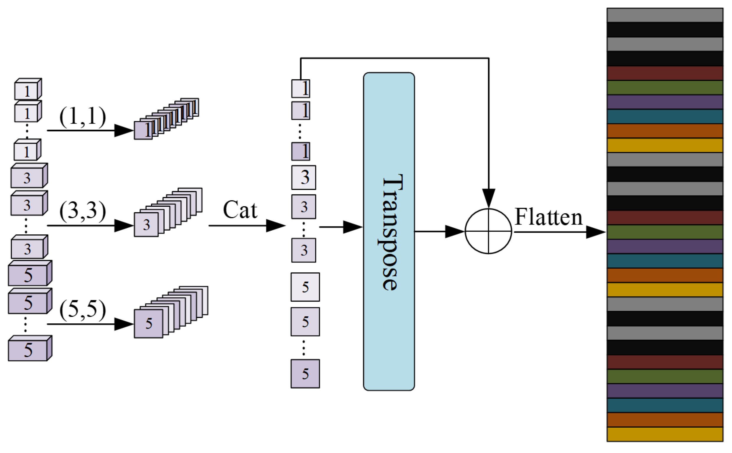
We have designed three 3D convolution kernels [36] with different sizes to extract the spectral–spatial information: (1, 1, 1), (3, 3, 3), and (5, 5, 5). When using a 1-sized convolution kernel, the padding is set to 0. For a 3-sized convolution kernel, the padding is set to 1, and for a 5-sized convolution kernel, the padding is set to 2. These convolution kernels are then applied to extract features from the preprocessed dataset, denoted as $X_{in}$. Afterward, the 3D feature sequences obtained from each of the three convolution kernels are concatenated. This operation enhances the preserved components and incorporates the sequence information of varying sizes, thereby increasing the richness of the features. The expanded multiscale feature information is subsequently fed into the spatial feature extraction layer.

2.2. Spatial Transpose Inception Module

To optimize the extraction and enrichment of HSI spatial features, we design three 2D convolution kernels with varying sizes: (1, 1), (5, 5), and (7, 7). For the 1-sized convolution kernel, the padding is set to 0. For the 3-sized convolution kernel, the padding is set to 1, and for the 5-sized convolution kernel, the padding is set to 2.

These three 2D convolution kernels are then applied to the output $X_{3D\_out}$ from the previous layer to extract the features. The 2D feature sequences obtained from each of the three convolution kernels are concatenated to further enhance the acquired spatial information. This can be expressed mathematically as follows:

$$X_{2D\_out}=\left\{\begin{array}{cc}Conv2D(X_{out},k=(1,1),p=0)& \\ Conv2D(X_{out},k=(5,5),p=1)& \\ Conv2D(X_{out},k=(7,7),p=2)\end{array}\right.$$

(2)

To enhance the input feature information in the transformer model, we utilize transpose convolution [37]. This technique aids in reconstructing and facilitating the transmission of feature information within the network. The output of the transpose convolution is subsequently connected to the 3D Inception module. A visual representation of this connection is illustrated in Figure 2 below.

The 3D Inception module generates eight feature cubes per layer, each with dimensions of $30\times 13\times 13$, resulting in an overall size of $8\times 30\times 13\times 13$. To align the dimensions, these cubes are stitched together in the fourth dimension, resulting in a size of $8\times 30\times 13\times 39$. However, the desired output dimension for the two-dimensional Inception module is three dimensional. To accommodate this, the sequence obtained after the stitching process is adjusted to (240, 13, 39). Each layer of the 2D Inception module generates 64 feature patches with dimensions of $13\times 39$, resulting in a size of $64\times 13\times 39$. These patches are then concatenated in the second dimension, resulting in a final size of $64\times 39\times 39$.

We maintain the feature dimensions as $64\times 39\times 39$ after applying the transpose convolution, and we ensure that the dimensions remain unchanged by connecting the transpose output with the first 2D convolution output. Finally, feature labeling is accomplished by flattening the feature sequence acquired from the transposed 2D Inception output.

2.3. Positional Embedding

To comprehensively describe the features of ground objects, we semantically label the features extracted by the Inception module. Given a feature map X, we can obtain the corresponding semantic label T by using the following formula:

$$X_{2D}^{L2}=Cat\left(TranpInception2D\left(X_{3D}^{L1}\right)\right)$$

(3)

$$X_{Incep}^{L3}=T\left(Flatten\left(X_{2D}^{L2}\right)\right)$$

(4)

$$X_{Incep}^{L3}=T\left(Flatten\left(X_{2D}^{L2}\right)\right)$$

(5)

$$X_{W_a}^L=softmax\left(T(X_{Incep}^{L3}•W_{aL})\right)$$

(6)

$$X_{W_b}^L=X_{Incep}^{L3}•W_{bL}$$

(7)

$$X_{cls}^L=X_{W_a}^L•X_{W_b}^L$$

(8)

where $X_{patch}^L\in R^{13\times 13\times C}$; $T(•)$ is a transposed function; $W_{aL}$, $W_{bL}$ represent a weight matrix initialized with a normal distribution; $X_{Incep}^{L3}$ and $W_{al}$ are dotted to map features $X_{patch}^L$ to the semantic group; and $X_{Incep}^{L3}$ and $W_{bl}$ are dotted to the semantic group.

Geographic information is arranged in spectral order. The location and order are very important. Similarly, the position and order of the features extracted by the Inception module are also very important.

$$P{E}_{pos,2i}=sin(pos/{1000}^{2i/d_{model}})$$

(9)

$$P{E}_{pos,2i+1}=cos(pos/{1000}^{2i/d_{model}})$$

(10)

In the formula, pos represents the location and i represents a dimension. Each dimension of position coding corresponds to a sinusoidal curve. While the relative position calculated using sine and cosine is linear, the relative position direction may be lost. To address this, we employ a coding mechanism that utilizes sine and cosine functions to record the relative position between feature semantics. This encoding mechanism helps capture the spatial relationships between different features.

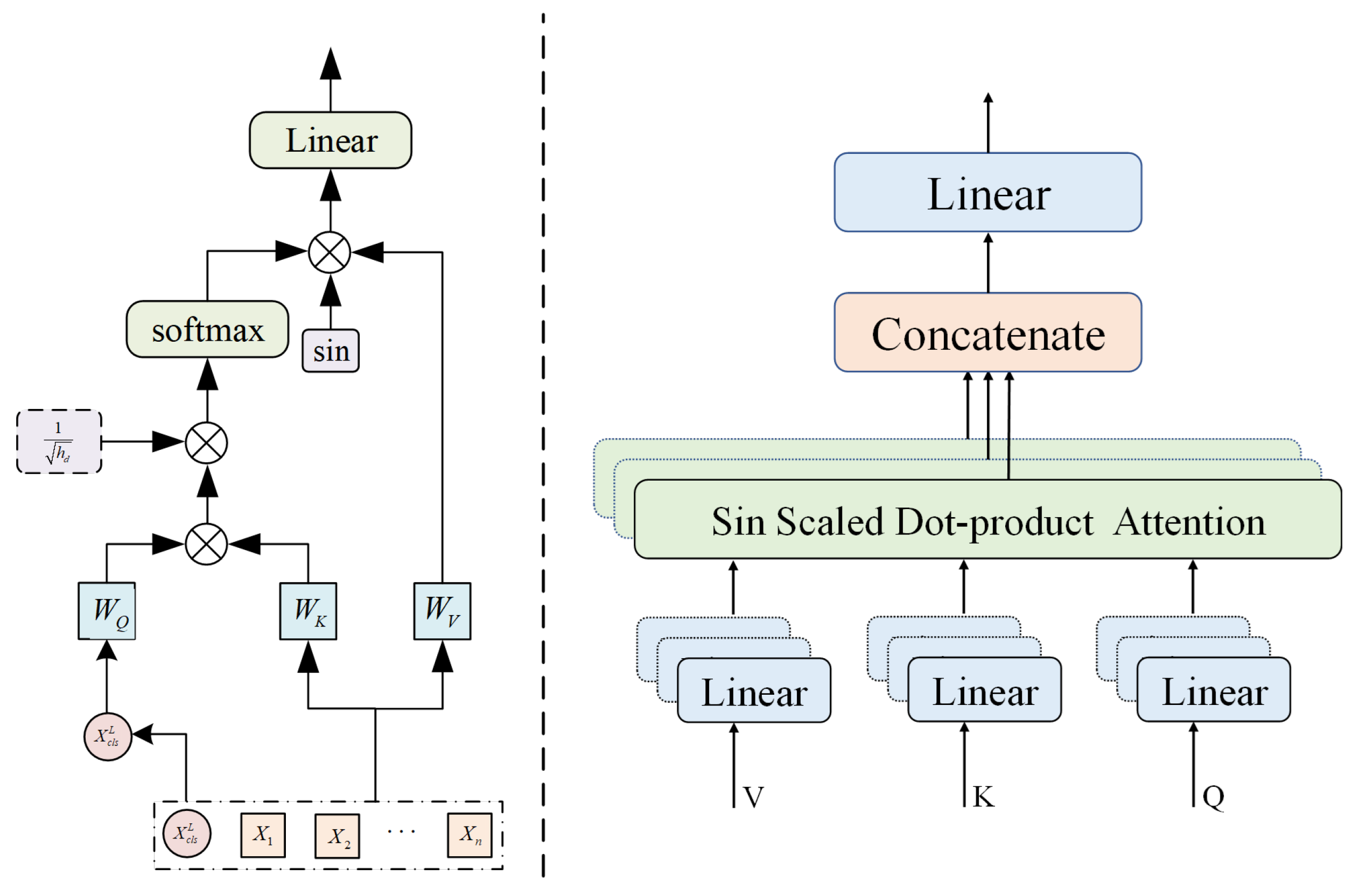
2.4. HSI Multi-Heads Cross-Sin Attention

The $X_{cls}^L$ tokens have a crucial role in learning the abstract representation of the entire HSI patch by exchanging information among themselves. This process takes place within the transformer architecture. The encoded $X_{cls}^L$ tokens are input into the transformer encoder, which consists of six stacked layers. Each layer comprises two sub-layers.

After normalization, the $X_{cls}^L$ tokens are passed through the attention layer. In this layer, the key and value components form a source. By comparing the query with each key, the similarity between them is calculated to determine the weight coefficient of the corresponding value for each key. The weighted sum of the values is then computed to obtain the final attention score. The specific implementation of this process is as follows:

$$Attention(Q,K,V)=softmax\left(\frac{Q{K}^T}{\sqrt{d_k}}\right)V$$

(11)

The variables Q, K, and V correspond to query, key, and value, respectively. To prevent the dot product of Q, K, and V from becoming too large, the softmax function is shifted to the region with a minimal gradient. In this design, a sine function is employed to constrain the dot product of Q, K, and V, as illustrated in the following formula:

$$Attention(Q,K,V)=softmax\left(sin\frac{Q{K}^T}{\sqrt{d_k}}\right)V$$

(12)

The average of a single attention head can suppress information from different positions and representation subspaces. One head is likely to extract features from a limited region. In contrast, multiple heads can simultaneously extract features from a particular region and take averages, which is more effective for extracting important information. Linear projections of Q, K, and V h times allow the model to jointly extract information from different positions and representation subspaces.

$$MultiHeadsin(Q,K,V)=Concat(hea{d}_1,\cdots ,hea{d}_n)W^o$$

(13)

$$hea{d}_i=sinAttention(Q{W}_i^Q,K{W}_i^K,V{W}_i^V)$$

(14)

Furthermore, multiple sinusoidal attention heads are employed for feature extraction. The attention weights generated by each head are combined by concatenation and then multiplied with their respective weight matrix to yield the ultimate attention coefficients. This approach facilitates the amalgamation of information from multiple heads, thereby enriching the overall representation and capturing diverse aspects of the input data. The schematic diagram is shown in Figure 3 below.

The figure illustrates the linear transformation of the feature sequence to obtain Q, K, and V. It calculates the relevance between the Q of the current sequence and the key information K of itself, as well as the relevance between the Q of the current sequence and the key information K of other sequences, resulting in the correlation coefficients between the current sequence and other sequences. In the case of multiple attention heads, the correlation operation is performed multiple times on the same Q to obtain multiple sets of attention coefficients, which are then averaged. The correlation coefficients of each sequence, when multiplied with their respective V, yield the final attention matrix. To ensure that the output falls within the activation region of the activation function, a sine function constraint is added to the dot product between Q and V during the final multiplication. The left part of the figure describes the computation process of the multi-head attention mechanism, while the right part provides an illustration of the multi-head attention mechanism.

The denominator of the dot product of Q and K in cross-sin multi-head attention is $\sqrt{h_d}$, where $h_d$ = embedding dimension/number of heads. The Q, K, and V scaling dot product operation adds a sine to limit the dot product range. As shown in the self-focus module, if the number of headers exceeds one, Cross sin AT will become a multi header cross focus, and when doing so, it can be represented as MCross-sinAT.

3. Experimental Results

Large networks and training datasets can result in a proliferation of model parameters and extended computation time, thereby impeding the implementation and adoption of the algorithm. Consequently, a major objective of this algorithm was to minimize the model parameters and training sets while upholding high-precision classification outcomes. To ascertain the feasibility and advancement of the proposed approach, verification and comparative tests were conducted on three publicly accessible datasets: India Pine, Pavia University, and Salinas. These tests were designed to assess the efficacy and performance of the algorithm vis-à-vis existing methods.

3.1. Hyperspectral Dataset

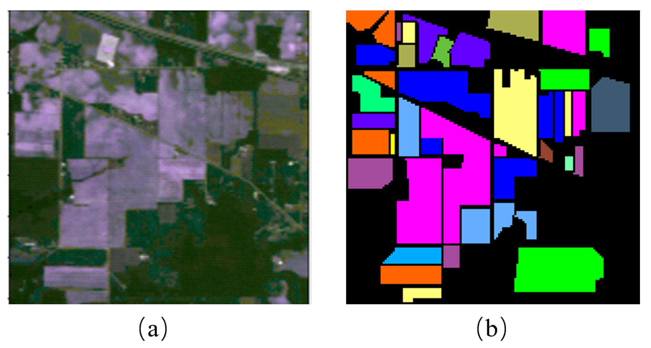
The India Pines dataset contains imaging data captured by AVRIS sensors at a designated testing site in northwest Indiana, with a specific emphasis on Indian pine vegetation. The dataset consists of 145 × 145 pixels and incorporates 224 spectral reflection bands after excluding 20 water absorption bands and noise bands. It possesses a spatial resolution of 20 m and encompasses 16 distinct land cover categories. To visually illustrate the underlying surface, Figure 4 depicts both true and pseudo-colored mappings. For convenience,

Table 1. Experimental training and test dataset: India Pines/Pavia University/Salinas.

	India Pines		Pavia University		Salinas
	class	total	class	total	class	total
1	Alfalfa	46	Asphalt	6631	Brocoli_green_weeds_1	2009
2	Corn-notill	1428	Meadows	18,649	Brocoli_green_weeds_2	3726
3	Corn-mintill	830	Gravel	2099	Fallow	1976
4	Corn	237	Trees	3064	Fallow_rough_plow	1394
5	Grass-pasture	483	Metal	1345	Fallow_smooth	2678
6	Grass-trees	730	Bare Soil	5029	Stubble	3959
7	Grass-pasture-mowed	28	Bitumen	1330	Celery	3579
8	Hay-windrowed	478	Bricks	1330	Grapes_untrained	11,271
9	Oats	20	Shadows	947	Soil_vinyard_develop	6203
10	Soybean-notill	972			Corn_senesced_green_weeds	3278
11	Soybean-mintill	2455			Lettuce_romaine_4wk	1068
12	Soybean-clean	593			Lettuce_romaine_5wk	1927
13	Wheat	205			Lettuce_romaine_6wk	916
14	Woods	1265			Lettuce_romaine_7wk	1070
15	Buildings-Grass-Trees-Drives	386			Vinyard_untrained	7268
16	Stone-Steel-Towers	93			Vinyard_vertical_trellis	1807
total		10,249		42,276		54,129
Training/Test	Training = 0.05 Test = 0.95

provides a comprehensive list of the specific land cover categories that are included in the India Pines dataset.

The Pavia University dataset consists of imaging data gathered by ROSIS sensors at the University of Pavia. It encompasses 610 × 340 pixels and comprises 103 spectral bands after excluding 12 noise bands. The dataset has a spatial resolution of 1.3 m and includes nine distinct land cover categories. Figure 5 presents a visual depiction of the bottom surface using both true and pseudo-color mapping. Additionally, Table 1 offers an exhaustive list of the specific land cover categories incorporated in the Pavia University dataset.

The Salinas dataset comprises imaging data captured by AVIRIS sensors over the Salinas Valley in California, USA. It encompasses 512 × 217 pixels and contains 204 frequency bands after eliminating 20 frequency bands with a low signal-to-noise ratio. With a spatial resolution of 3.7 m, it encompasses 16 distinct land cover categories. Figure 5 illustrates a true and pseudo-color map representing the bottom surface, while Table 1 provides a comprehensive list of the land cover categories included in the Salinas dataset.

3.2. Experimental Setting

(1) Evaluation metrics: To quantitatively assess the efficacy of this method and other methods, four evaluation metrics were employed: the overall accuracy (OA), average accuracy (AA), kappa coefficient (k), and individual classification accuracies for each land cover category. A higher value for each metric signifies a superior classification performance of the method.

(2) Machine configuration: The hardware configuration was an AMD Ryzen 7 5800 h CPU, an NVIDIA GeForce RTX 3060 graphics card, and 32 GB of memory. This machine is called the Lenovo R9000P, a wireless router product of China’s Lenovo Group, headquartered in Beijing, China. The software configuration included implementing all experiments using the PyTorch framework, a deep learning framework developed by the Facebook AI Research team. The programming language used for writing the programs is Python 3.8, which was developed by Dutch computer scientist Guido van Rossum in the early 1990s. The network parameters were set with Adam as the initial optimizer, and the initial learning rate was set to 0.001. Batch learning was employed with a batch size of 128, and each dataset was trained for 1000 epochs. The model parameters with the highest classification accuracy were saved.

3.3. Parameter Setting

In the parameter analysis, we investigated various parameters that impacted the classification performance and computational time of the network. Specifically, we concentrated on the input cube size, the configuration of the spectral convolution layer, and the layout of the spatial convolution layer. In order to determine the most suitable parameters for our experiments, we conducted relevant experiments. For additional information on the remaining parameter settings, please refer to Section 3.2.

Figure 6 depicts the framework for five sets of experiments, which employed patch sizes of 9, 11, 13, 15, and 17. These experiments were performed on the India Pines, Pavia University, and Salinas datasets to explore the optimal parameters.

As shown in Figure 6, it is evident that different patch sizes have an impact on the accuracy of ground object recognition by the network. Specifically, a larger patch size is associated with higher classification accuracy. Notably, when the patch size is set to 13, there are notable improvements in accuracy across the three datasets. However, increasing the patch size beyond 13 does not result in further enhancements in classification accuracy. From an operational perspective, opting for a smaller patch size allows for a faster computational speed. Therefore, we determined the final experimental patch size to be 13.

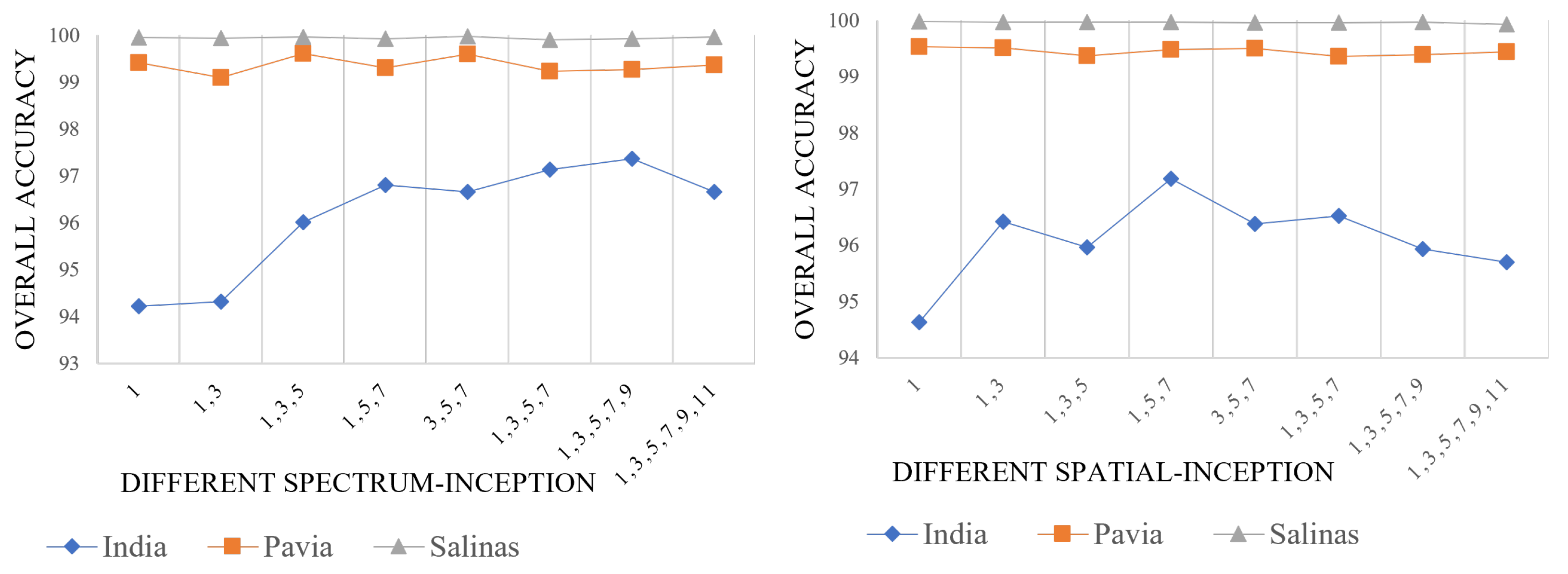
To extract the spectral and spatial features from hyperspectral images, we developed eight distinct sets of spectral and spatial Inception modules. These modules were utilized for feature extraction in our experiments. The experimental results were then evaluated using three datasets: India Pines, Pavia University, and Salinas. The depiction of the experimental outcomes can be observed in Figure 7.

Figure 7 demonstrates the impact of the spectral and spatial Inception modules, which consist of different sizes of 3D and 2D convolution kernels, on classification accuracy. In terms of spectral Inception, variations in module sizes have a noticeable effect on the classification of the India dataset. Within a specific range, larger Inception modules yield higher classification accuracy. The impact on the Pavia and Salinas datasets shows minor fluctuations. In order to maintain accuracy while improving computational efficiency, a spectral Inception composed of 3D convolution kernels with scales of 3, 5, and 7 was selected to extract the spectral information from the HSI.

As for spatial Inception, different-sized modules have a significant effect on the classification accuracy of the India dataset. However, once their convolution combinations exceed a certain size, the classification accuracy tends to decrease. Similar slight fluctuations are observed for the impact on the Pavia and Salinas datasets. Taking into account the need to maintain accuracy while improving the model’s running speed, a spatial Inception composed of 2D convolution kernels with scales of 1, 5, and 7 was chosen to extract the spatial information from the HSI.

Based on the aforementioned comparative experiments, we determined that setting the patch size of the multiscale CNN-transformer network to 13 × 13 yielded the optimal classification performance. For the spectral Inception module, it was found that using 3D convolution kernels at scales 3, 5, and 7 produced the best results. Similarly, for the spatial Inception module, employing 2D convolution kernels at scales 1, 5, and 7 proved to be the most effective. As a result of these configurations, the classification outcomes are shown in

Table 2. Classification results of transposed CNN-transformer setting optimal parameters.

Dataset	India Pines	Pavia University	Salinas
overall accuracy (OA)	97.19	99.49	99.97
average accuracy (AA)	96.93	98.96	99.97
kappa coefficient (K)	96.79	99.32	99.92

.

The data in the table represent the percentage of correct classifications, where a larger value indicates a better classification performance and more correctly classified samples.

3.4. Spatial Transposed Inception and Multi-Head Cross-Sin Attention Comparison Experiment

In order to independently validate the improvements brought by the spatial Inception module and the multi-head cross-sin attention module, we conducted a comparative study using a controlled variable approach. We treated the spatial Inception module and the multi-head cross-sin attention module as variables while keeping the other parameters constant. By adjusting the inclusion of these modules in the network and evaluating the results on three commonly used datasets, we obtained the validation outcomes presented in Figure 8 below.

Figure 8 illustrates the results of our experiments. In (a), the left column shows the experimental outcomes without the spatial Inception module, while the right column displays the outcomes with the inclusion of the spatial Inception module. It is evident that the network utilizing the spatial Inception module achieved higher classification accuracy, demonstrating the superiority of this module. Similarly, in (b), the left column presents the experimental results without the multi-head cross-sin attention module, while the right column exhibits the results with the multi-head cross-sin attention module. It can be concluded that the network incorporating the multi-head cross-sin attention module achieves superior classification performance, confirming the improvements brought by this module.

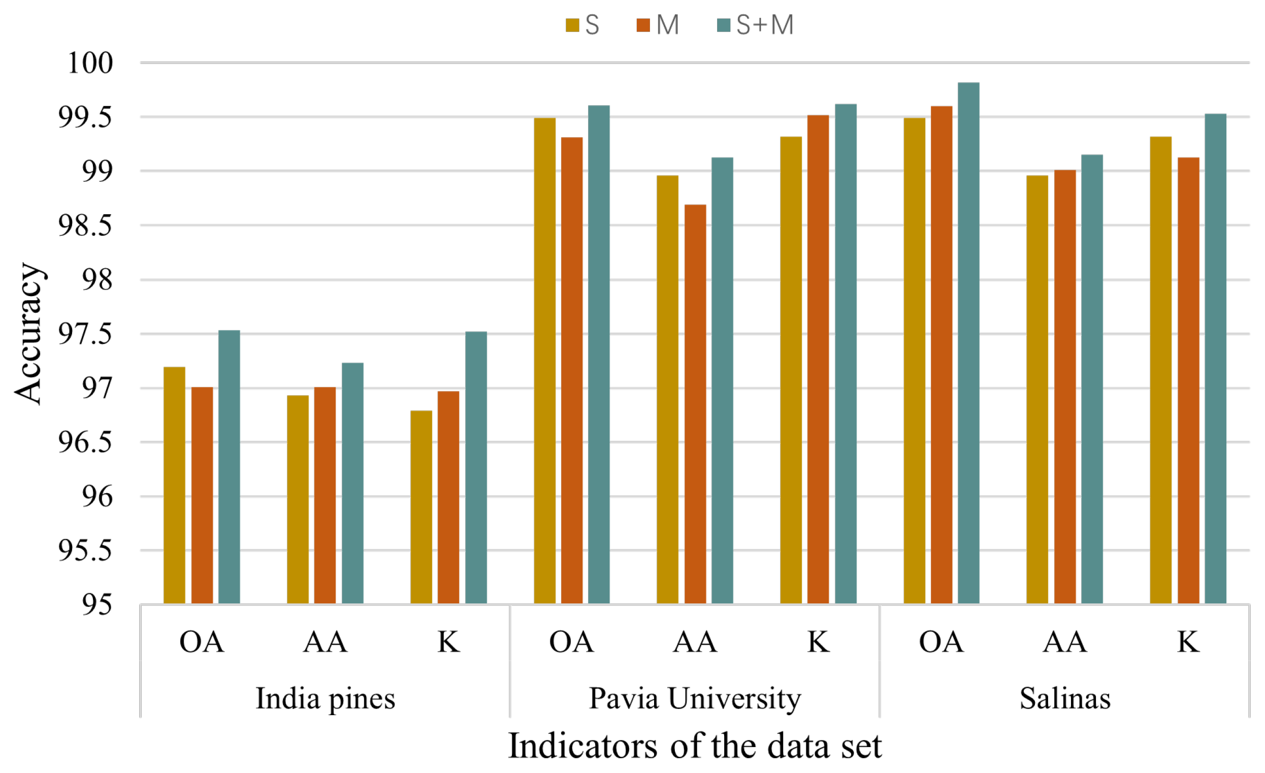
The results presented in Figure 9 demonstrate that the simultaneous inclusion of both the spatial transposed Inception and multi-head cross-sin attention modules has a positive impact on classification performance. Specifically, it leads to enhancements in the overall classification accuracy and average classification accuracy, as well as other metrics.

3.5. Comparison of Different Network Classification Results

In order to demonstrate the effectiveness of the proposed method in this study, we conducted comparative experiments on three datasets: India Pines, Pavia University, and Salinas. By analyzing and comparing the classification accuracy of the SSTN [38], SSRN [39], SSFTT, and MSSTT, we further substantiated the novelty and innovation of the method presented in this paper. The results of the comparative experiments can be summarized as follows.

Table 3. Classification accuracy of different methods on the India Pines dataset.

Method	SSTN	SSRN	SSFTT	MSSTT
OA (%)	95.13	87.59	96.31	97.19
AA (%)	91.70	89.07	92.17	96.93
Kappa (%)	94.44	85.75	95.79	96.79
Alfalfa	85.00	92.50	88.46	90.46
Corn-notill	96.51	88.62	97.89	97.89
Corn-mintill	92.89	77.63	95.71	95.71
Corn	89.49	80.82	98.17	98.17
Grass-pasture	95.69	89.03	98.29	98.29
Grass-trees	100	92.43	97.58	97.58
Grass-pasture-mowed	95.06	98.16	96.43	96.43
Hay-windrowed	96.91	94.54	98.06	98.06
Oats	91.87	99.16	99.89	100
Soybean-notill	96.66	83.52	94.73	94.73
Soybean-mintill	88.35	90.52	96.60	96.60
Soybean-clean	100	100	99.21	99.21
Wheat	98.99	98.97	99.48	99.8
Woods	93.26	99.32	97.79	97.79
Buildings-Grass-Trees-Drives	93.25	85.39	99.41	99.41
Stone-Steel-Towers	98.82	98.82	95.45	95.45

presents the overall accuracy (OA) of the SSTN, SSRN, SSFTT, and MSSTT methods for the OA, average accuracy (AA), Kappa coefficient (Kaappa), and individual ground features in the India Pines dataset. The data in the table represent the percentage of correct classifications, where a larger value indicates a better classification performance and more correctly classified samples. It is evident that the MSSTT approach proposed in this study outperforms the other three methods in terms of classification accuracy. The classification results are visualized in Figure 10.

From Figure 10, it can be observed that compared to the ground truth image, SSTN and SSRN exhibit errors in multiple land cover classifications. SSFTT shows some improvement in classification performance compared to the previous two methods but still exhibits errors in various land cover categories, such as Corn-notill and Soybean-notill. The proposed method, MSSTT, generates a final classification map that is closest to the ground truth image.

Table 4. Classification accuracy of different methods on Pavia University dataset.

Method	SSTN	SSRN	SSFTT	MSSTT
OA (%)	97.67	95.98	99.31	99.47
AA (%)	96.81	95.54	98.66	98.86
Kappa (%)	96.92	94.69	98.89	99.29
Asphalt	97.94	98.81	99.45	99.51
Meadows	99.49	96.44	99.99	99.77
Gravel	92.62	79.60	99.40	99.09
Trees	90.22	96.31	98.78	98.32
Metal sheets	99.77	99.92	100	100
Bare Soil	99.66	96.62	99.96	99.73
Bitumen	99.69	99.16	99.76	99.84
Bricks	92.39	93.13	98.17	98.60
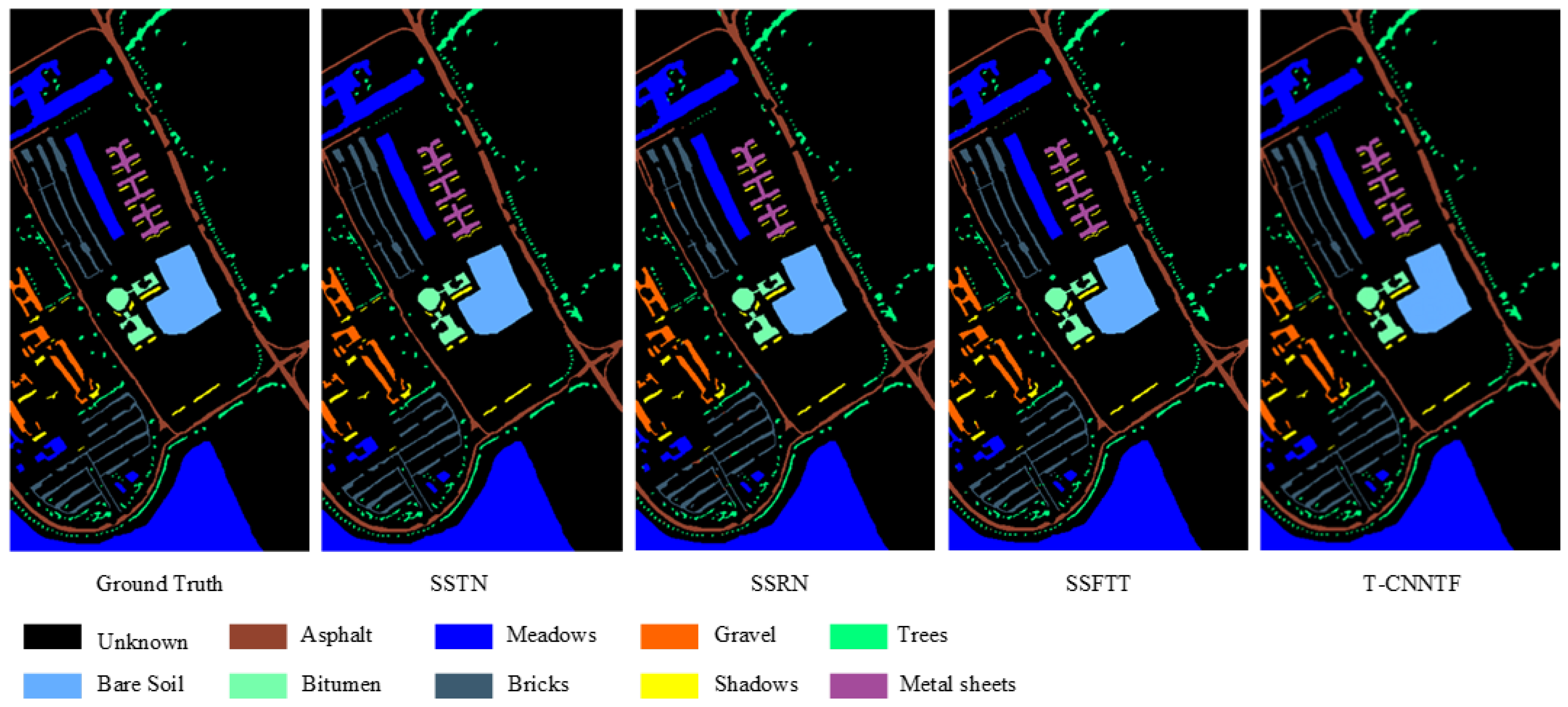
Shadows	99.46	99.89	96.93	98.40

presents the overall accuracy (OA) of the SSTN, SSRN, SSFTT, and MSSTT methods for the OA, average accuracy (AA), Kappa coefficient (Kappa), and individual ground features in the Pavia University dataset. The data in the table represent the percentage of correct classification, where a larger value indicates a better classification performance and more correctly classified samples. It is evident that the MSSTT approach proposed in this study outperforms the other three methods in terms of classification accuracy. The classification results are visualized in Figure 11.

From Figure 11, it can be observed that compared to the ground truth image, SSTN exhibits errors in multiple land cover classifications, such as Bare Soil and Bricks. SSRN also exhibits errors in the classification of Bricks. SSFTT shows errors in multiple land cover categories, such as Gravel and Shadows. The proposed method, MSSTT, generates a final classification map that is closest to the ground truth image.

Table 5. Classification accuracy of different methods on Salinas dataset.

Method	SSTN	SSRN	SSFTT	MSSTT
OA (%)	88.38	88.70	98.95	99.90
AA (%)	94.51	94.05	98.90	99.89
Kappa (%)	87.06	87.37	98.95	99.89
Brocoli_green_weeds_1	95.86	93.11	100	100
Brocoli_green_weeds_2	99.20	99.17	100	100
Fallow	100	99.21	99.89	100
Fallow_rough_plow	99.56	98.41	99.32	99.17
Fallow_smooth	97.50	97.84	98.18	98.99
Stubble	99.39	98.69	99.97	100
Celery	98.71	98.57	100	100
Grapes_untrained	73.65	82.34	99.81	100
Soil_vinyard_develop	99.52	100	100	99.98
Corn_senesced-green_weeds	96.87	97.46	98.81	99.74
Lettuce_romaine_4wk	98.66	99.88	99.49	100
Lettuce_romaine_5wk	99.09	98.66	98.99	99.89
Lettuce_romaine_6wk	98.89	98.11	100	100
Lettuce_romaine_7wk	99.29	99.49	99.61	100
Vinyard_untrained	63.12	53.41	100	99.99
Vinyard_vertical_trellis	91.99	89.32	100	100

presents the overall accuracy (OA) of the SSTN, SSRN, SSFTT, and MSSTT methods for the OA, average accuracy (AA), Kappa coefficient (Kappa), and individual ground features in the Salinas dataset. The data in the table represent the percentage of correct classification, where a larger value indicates a better classification performance and more correctly classified samples. It is evident that the MSSTT approach proposed in this study outperforms the other three methods in terms of classification accuracy. The classification results are visualized in Figure 12.

From Figure 12, it can be observed that compared to the ground truth image, SSTN, SSRN, and SSFTT all exhibit errors in the classification of Grapes untrained. The proposed method, MSSTT, generates a final classification map that is closest to the ground truth image.

The classification visualization results of SSTN, SSRN, SSFTT, and MSSTT on the India Pines, Pavia University, and Salinas datasets are depicted in Figure 10, Figure 11 and Figure 12. Among these methods, the classification result map obtained using MSSTT exhibits the cleanest and most accurate alignment with the ground reality map. Conversely, the results of SSTN, SSRN, and SSFTT display noticeable noise across all three datasets. Specifically, on the India Pines dataset, SSTN, SSRN, and SSFTT demonstrate relatively poor classification performance for the blue, yellow, and pink regions in the middle. In contrast, the proposed method in this study significantly improves the identification of these three color regions. On the Pavia University dataset, SSTN misidentifies the light blue area, SSRN incorrectly classifies the middle dark gray area as dark brown, and SSFTT misclassifies the brown area in the lower left corner as yellow. In contrast, the MSSTT approach performs closest to the actual ground image in terms of accurate identification. Regarding the Salinas dataset, SSTN and SSRN both misidentify the middle gray area, while SSFTT misclassifies the green area. In comparison, the recognition by MSSTT is almost identical to the real ground image.

These observations lead to the conclusion that the method proposed in this paper maintains optimal boundary regions, further validating the classification performance of MSSTT.

4. Conclusions

This paper presents an MSSTT method designed to improve the performance of hyperspectral image (HSI) classification. The proposed approach combines a spectral Inception module, which utilizes 3D convolution kernels, and a spatial transposed Inception module, which utilizes 2D convolution kernels. These modules are integrated with a transformer. The spectral Inception module is responsible for extracting spectral features, while the spatial transposed Inception module focuses on extracting spatial features. Both modules work together to expand the feature space for semantic annotation. Additionally, to ensure that the attention output remains within the valid range of the activation function, a limitation operation is employed in the attention mechanism.

Our work can be applied in fields such as plant pest detection and geological exploration. The reflectance spectral properties of healthy plants and those affected by pests and diseases are different, and the more accurate the land classification is, the more accurate the detection of pests and diseases will be. For geological exploration, this method can greatly reduce human and time costs by using satellite images to classify ground features.

This study has demonstrated the superiority of combining variants of different dimensions with transformers and has made progress in extracting HSI spectral and spatial features. However, there may still be redundancies or the loss of feature information in the dimensionality reduction process. Based on this, our future work will focus on further exploring HSI spectral and spatial feature extraction and postprocessing after land classification. We also plan to deploy this method on hardware for accelerated processing, further improving the classification accuracy and reducing the model size.