1. Introduction
In recent years, the need to recognize a person’s emotions has increased, and there has been a growing interest in human emotion recognition across various fields, including brain–computer interfaces [
1,
2], assistance [
3], medicine [
4], psychology [
5,
6], and marketing [
7]. Facial expressions are one of the primary nonverbal means of conveying emotion and play an important role in everyday human communication. According to a seminal paper [
8], more than half of the messages related to feelings and attitudes are contained in facial expressions. Emotions are continuous in nature. However, it is common to measure them on a discrete scale. Ekman and Friesen [
9] identified six universal emotions based on a study of people from different cultures. This study showed that people, regardless of their culture, perceive some basic emotions in the same way. These basic emotions are happiness, anger, disgust, sadness, surprise, and fear. Over time, critics of this model have emerged [
10], arguing that emotions are not universal and have a high cultural component; nevertheless, the model of the six basic emotions continues to be widely used in emotion recognition [
11].
In the last few decades, facial expression recognition (FER) has come a long way thanks to advances in computer vision and machine learning [
12]. Traditionally, feature-extraction algorithms such as scale-invariant feature transform or local binary patterns and classification algorithms such as support vector machines or artificial neural networks have been used for this task [
13,
14,
15]. However, the current trend is to use convolutional neural networks (CNNs), which perform feature extraction and classification at the same time [
16]. FER datasets can be divided into two main categories, depending on how the samples were obtained: laboratory-controlled or wild. In lab-controlled datasets, all images are taken under the same conditions. Therefore, there are no variations in illumination, occlusion, or pose. Under these conditions, it is relatively easy to achieve high classification accuracy without resorting to complex models; in fact, in some datasets, such as CK+ or JAFFE, 100% of the images can be correctly classified [
17,
18]. On the other hand, in-the-wild datasets contain images taken under uncontrolled conditions, such as those found in the real world. In this scenario, the classification accuracy is significantly lower than that obtained in laboratory-controlled datasets [
19,
20].
FER in-the-wild datasets typically contain images of many different sizes [
21], which are typically scaled to 224 × 224 to feed a neural network. The main drawback of training a CNN on images of this size is that, as the network infers lower-resolution images, classification accuracy drops significantly [
20]. There are many applications where obtaining high-resolution images of human faces is not feasible, for example when trying to determine the emotional state of multiple people simultaneously in large spaces such as shopping malls, parks, or airports. In these situations, each person is at a different distance from the camera, resulting in images of different resolutions. As highlighted in a survey [
22], these circumstances present a variety of challenges, including occlusion, pose, low resolution, scale variations, and variations in illumination levels. In addition, they underscore the importance of the efficiency of FER models when processing images of multiple people in real-time.
In these scenarios, a network trained on low-resolution images can be more robust because the network is less dependent on fine details that are not present in low-resolution images, thus increasing its ability to generalize. In addition, working with smaller images reduces the computational cost and bandwidth required to transfer the images from the cameras to the computer where they are processed. CNNs that work with low-resolution images are lighter because the features occupy less memory, making it possible to use methods such as ensemble learning, which is not widely used in deep learning due to its high computational complexity [
23]. Ensemble learning methods combine the results of multiple machine learning estimators with the goal of obtaining a model that generalizes better than the estimators of which it is composed [
24]. Assembling
n CNNs means multiplying by
n the number of trainable parameters of the model and the size of the features of each image in the network.
To illustrate the problem more clearly, let us consider a possible application scenario, such as a smart campus proposal, where FER is used to quantify the degree of user comfort [
25]. This environment uses a network of wireless cameras that send video to servers that recognize people’s faces and predict their emotions in real-time. In this environment, it is not possible to control the distance of building occupants from the camera, their position, or possible occlusions. In addition, there can be hundreds or even thousands of people in this type of environment, which means managing a huge flow of data. In this context, the resolution of the images is a fundamental variable: the lower the resolution of the images, the lower the workload of the system is. For this reason, the use of lightweight models specifically designed for processing low-resolution images in real-world conditions is of interest.
This paper proposes a model for facial expression recognition from low-resolution images based on a residual network and a voting strategy. This model tries to improve the generalization capability of the neural network by combining different classification results, as is done in ensemble methods, but without increasing the complexity of the model excessively. For this purpose, instead of using n networks to obtain n votes (predictions), n patches of each image are taken and fed into a single network, which provides the n votes based on which the class of the image is determined. Thus, the number of trainable parameters of the model remains constant regardless of the number of votes. If the image is partitioned into multiple patches before entering the network, the size of the image features is multiplied by n. To address this problem, our work explored different intermediate points in the network where partitioning can be performed. The closer the splitting point is to the network exit, the smaller the dimensionality of the image features and, consequently, the smaller the space required to store them. In this paper, the proposed approach was implemented on a residual network, although theoretically, this approach could be used with virtually any CNN.
The main contributions of this paper can be summarized as follows:
Integration of a voting mechanism: A voting mechanism is integrated into a residual network architecture to improve the accuracy of facial expression recognition in low-resolution images.
Retention of model size: The proposed voting approach does not increase the number of trainable parameters regardless of where the image is split. This differs from conventional ensemble model implementations, which tend to increase the number of trainable parameters.
Examination of split points: The method is evaluated by performing image splitting at different points in the network to determine the impact on network accuracy and forward pass size after applying the model. The closer the split point is to the network output, the lower the dimensionality of the image features and, thus, the smaller the space required to store them.
Experimental evaluation: Extensive experiments were performed on two public benchmark datasets (AffectNet and RAF-DB) to validate the effectiveness of the proposed method. The images of these datasets were resized to 48 × 48 px, which makes the proposed method very robust to variations in image resolution. The results showed that it is possible to reduce the resolution of the images used to train FER models without significant loss of accuracy.
The rest of this paper is organized as follows. In
Section 2, several existing algorithms for FER in the wild are discussed. The materials and methods used in this work are presented in
Section 3.
Section 4 contains the experimental results. Finally,
Section 5 draws the conclusions of the study.
3. Materials and Methods
The notations and symbols used in this article are shown in
Table 1.
3.1. Network Architecture
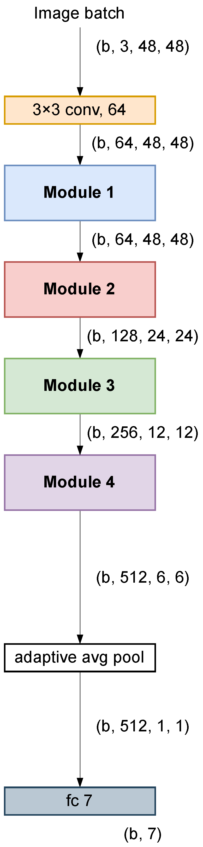
Our work used the ResNet-18 architecture for ImageNet [
48] as a baseline, with slight modifications to adapt it to smaller images (see
Figure 1). ResNet-18 is a lightweight and robust architecture that has demonstrated its superiority over other heavier architectures in computer vision tasks [
48]. This model has been widely used as the backbone for various models that have reached the state-of-the-art in FER in the wild [
49,
50,
51,
52,
53]. The skip connections in ResNet-18 allow faster convergence during training by providing shortcuts for gradient flow. This leads to faster training and often better generalization, especially when dealing with complex datasets. In addition, this model has a relatively simple and easily manipulated structure that allows the splitting and voting strategy presented in this paper to be easily incorporated at various points in the architecture.
In the original architecture, designed for images of 224 × 224 px, the first convolutional layer used a kernel of size 7 × 7 and a stride of two, followed by a max-pooling layer to reduce the dimensionality quickly. In our network, the input images had a size of 48 × 48 px, so it was not necessary to reduce the dimensionality so quickly. Therefore, we chose a 3 × 3 kernel in the first layer with a stride of one and removed the max-pooling layer. Otherwise, the baseline architecture was identical to the original.
We believe that the 7 × 7 kernel size in the original architecture may be excessive for 48 × 48 px images and may result in a loss of fine-grained features. The use of a 3 × 3 kernel is congruent with the ResNet approach for CIFAR, which is designed to work with 32 × 32 px images. On the other hand, the decision to eliminate the max-pooling layer was due to the fact that, for images with an input size of 48 × 48, the dimensionality at this point of the network is already low without the need to perform any pooling operation. In the original architecture, this layer allows reducing the dimensionality from 112 × 112 to 56 × 56. In our case, however, the dimensionality is 48 × 48.
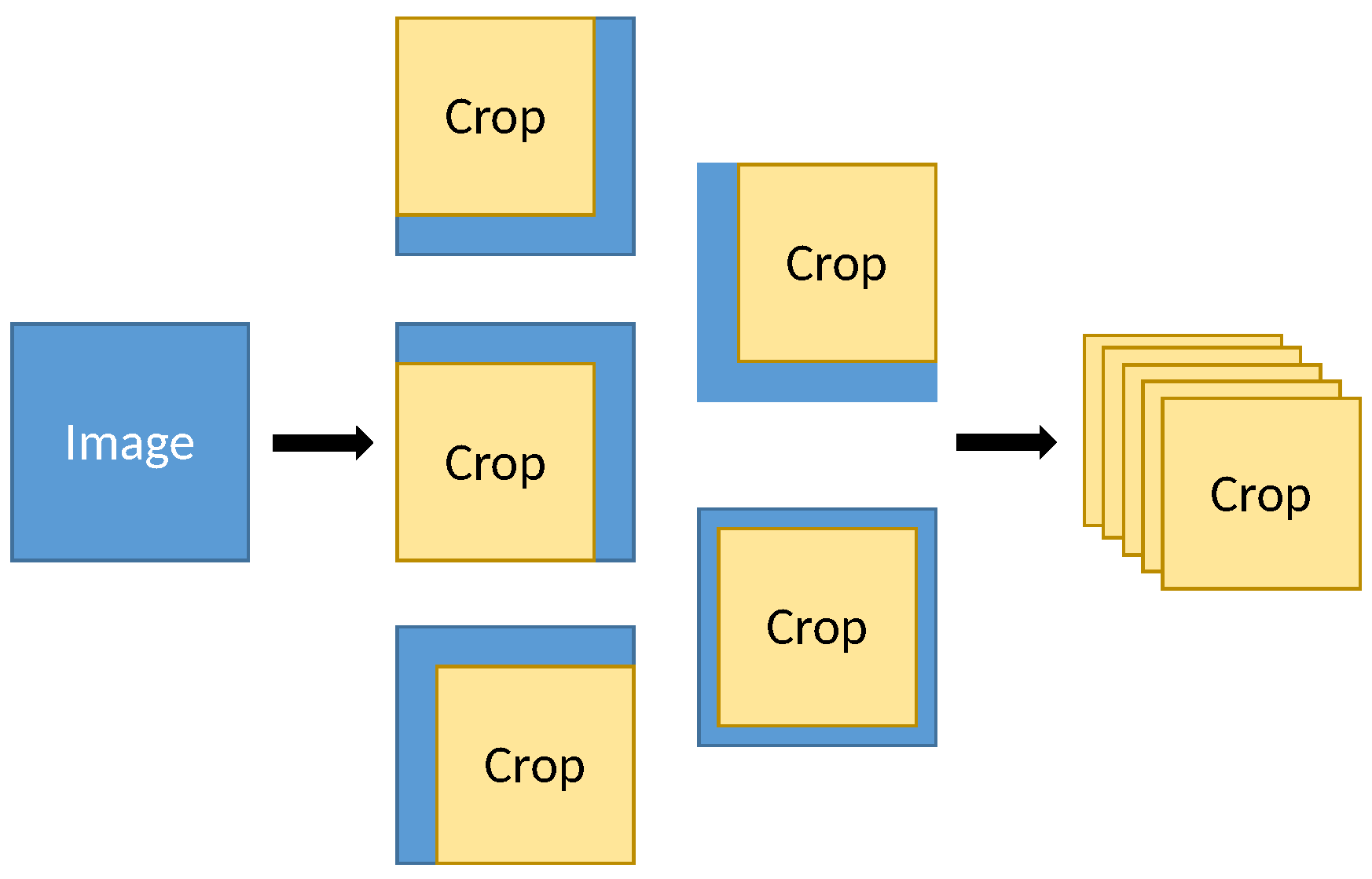
From the baseline architecture, three variants were developed by introducing a voting strategy. For this purpose, each image entering the network was cut into five overlapping square patches; the side dimension of each patch was 5/6 of the image side dimension, and one patch was taken at the center of the image and one at each corner of the image (see
Figure 2). Once the patches were obtained, a copy of the patches was made and mirrored horizontally. In this way, 10 sub-images were obtained from each image. The pseudocode of the image division process is shown in Algorithm 1.
Accurately recognizing facial expressions in real-world situations is challenging due to the variety of lighting conditions, poses, backgrounds, and occlusions. By dividing the image into multiple overlapping slices, we sought to increase the robustness and stability of the model by forcing it to work with incomplete and off-center images. This approach yields different predictions from the same image, as if it were an assembler model, but without the need for ten different neural networks. The choice of a 5/6 ratio for image cropping is based on the observation that this ratio preserves most of the facial area relevant to facial expressions in most images, while eliminating less-informative regions. In addition, the dimensions of the images produced by each module within the baseline architecture are all divisible by six, which simplifies the cropping procedure.
| Algorithm 1 Image patch generation |
- 1:
Input: Batch of images: x of shape (batch_size, num_channels, height, width) - 2:
Output: Patches: (batch_size × 10, num_channels, new_height, new_width) - 3:
Initialize an empty list - 4:
for each image in batch x do - 5:
Get dimensions of : , - 6:
Calculate new dimensions: , - 7:
for each patch position do - 8:
Calculate patch coordinates: , , , for the current position - 9:
Extract patch: - 10:
Add to - 11:
end for - 12:
Mirror horizontally: - 13:
for each patch position do - 14:
Calculate patch coordinates for mirrored image - 15:
Extract patch from mirrored image - 16:
Add mirrored to - 17:
end for - 18:
end for - 19:
Concatenate patches along the batch dimension:
|
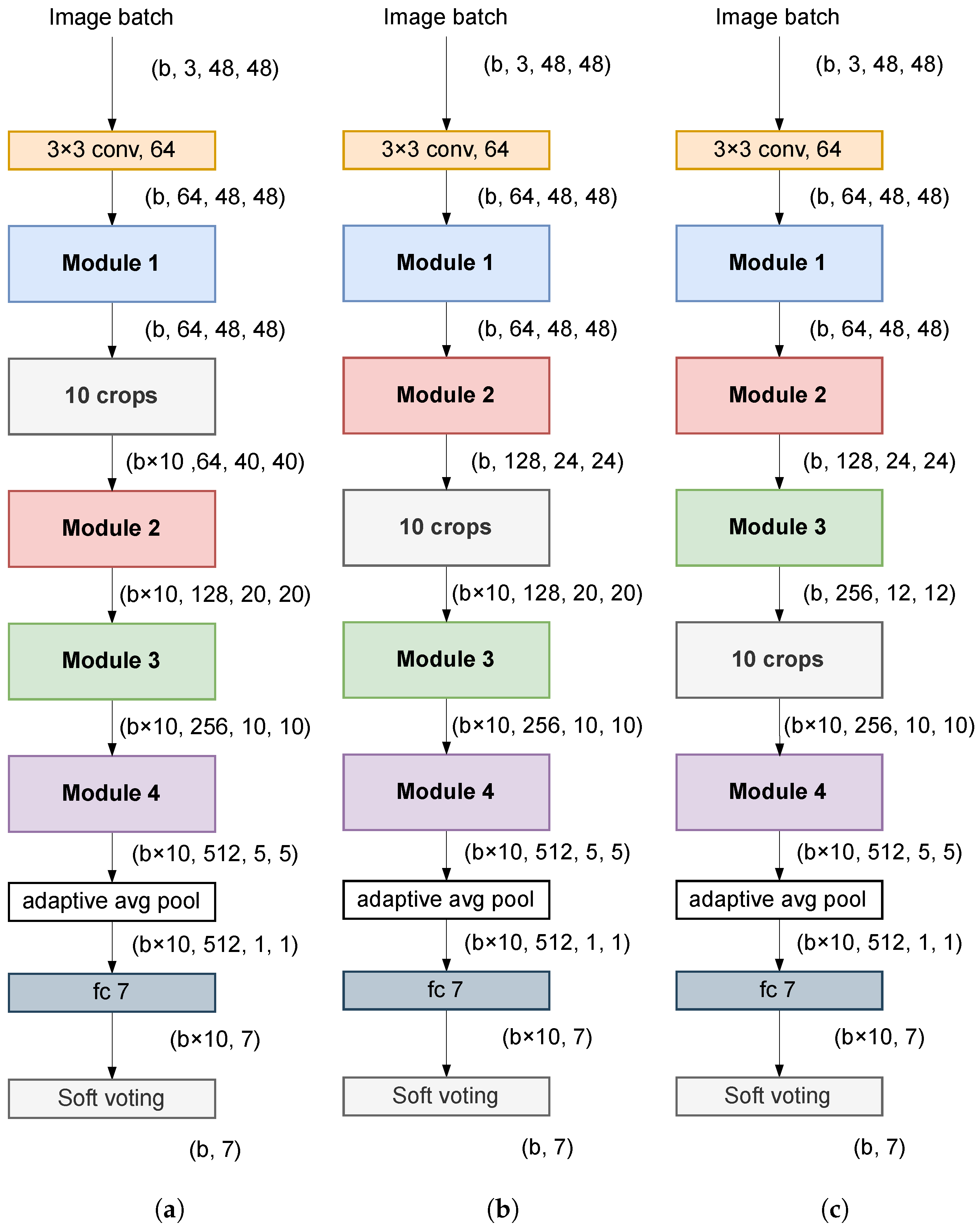
Cropping before entering the network would significantly increase the size of the image features within the network. For this reason, in this work, cropping was performed at an intermediate point in the network where the dimensionality is lower. Specifically, three points were examined (see
Figure 3), namely the output of Modules 1, 2, and 3. The output of the fully connected (FC) layer of the network provided the predictions of each of the 10 crops into which the image had been divided. The final prediction of the class to which the image belonged was obtained by calculating the average of these 10 predictions (soft voting). The closer the cropping point was to the input of the network, the larger the size of the images within the network (forward pass) and, consequently, the smaller the number of images that could be processed per batch in both training and inference.
Table 2 shows the estimated forward pass sizes per image of the proposed architecture, depending on where in the network the image was divided into 10 crops. Included also in the first row is the forward pass size that the baseline architecture would have if the image were split before entering the network. In this case, the effective forward pass size would be 70 MB because it would have to be multiplied by 10 since 10 sub-images would be used to predict each sample.
The forward pass size was measured by calculating the space occupied by the tensors on the graphics card before and after inserting a batch of images and dividing this value by the number of images in each batch. The occupied space was measured using the
function of PyTorch [
54].
3.2. Datasets
To evaluate the proposed method, two popular FER datasets in the wild were used, namely AffectNet [
55] and RAF-DB [
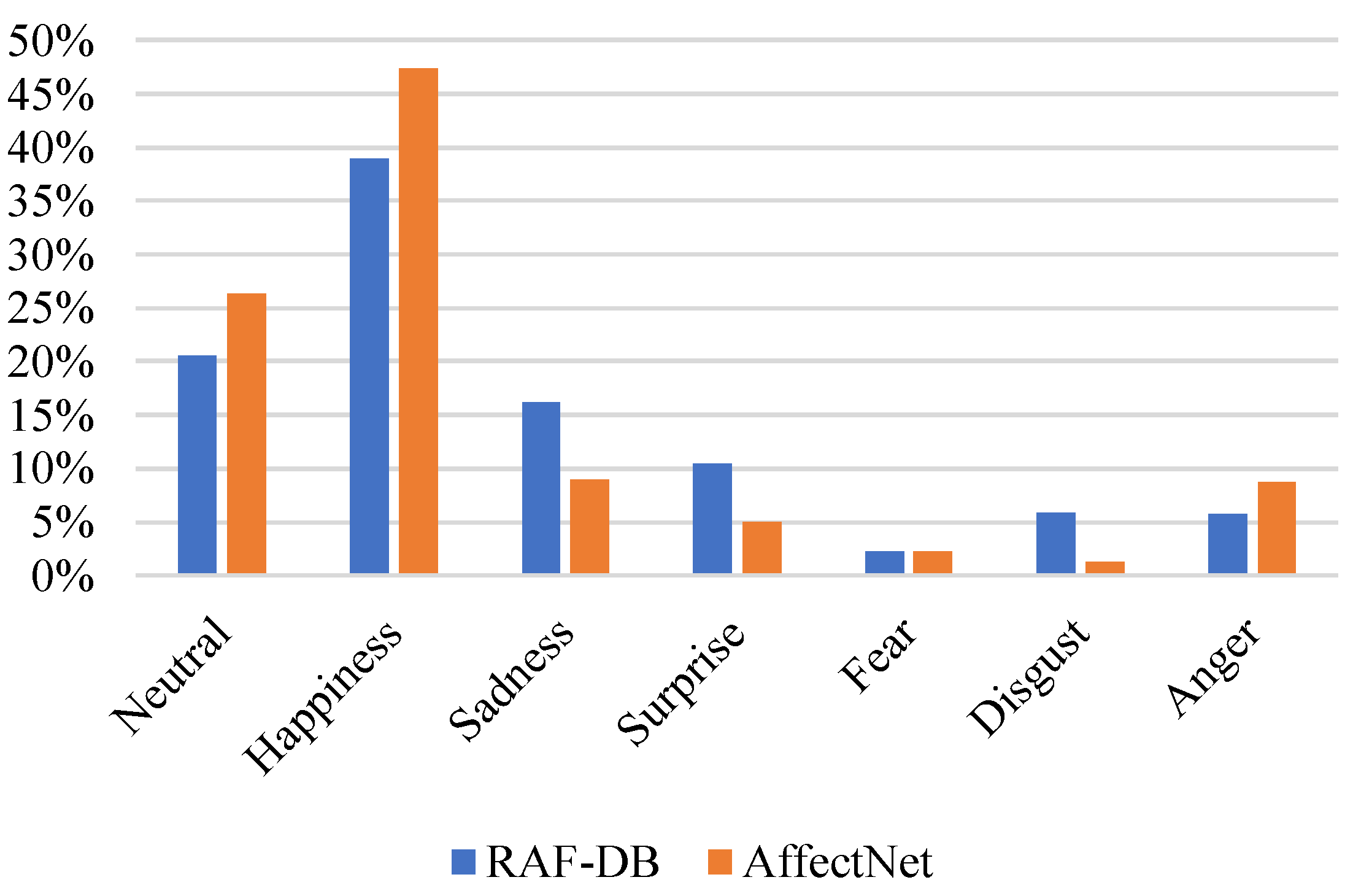
56]. These datasets contain images of different sizes taken under challenging conditions with occlusions and variations in illumination and pose. Both datasets are highly imbalanced.
Figure 4 shows the distribution of images in the original training set of the two datasets above.
3.2.1. AffectNet
AffectNet contains more than 440,000 facial images collected from the Internet by querying various search engines with 1250 emotion-related keywords in six different languages. Approximately 291,651 of these images were manually annotated for the presence of eight facial expressions (fear, happiness, sadness, neutral, anger, surprise, disgust, and contempt). In this work, the contempt expression was not used, so there was a total of 287,401 images, divided into two subsets, and 500 images of each class belonged to the validation set and the rest to the training set. Since the test set was not published by the authors, the validation set was used as the test set, and we created a new validation set by randomly taking 500 images from each class of the training set.
3.2.2. RAF-DB
The RAF-DB dataset contains 29,672 manually annotated images collected from the Internet, which are divided into two subsets according to the type of annotation: (i) basic expressions and (ii) compound expressions. Here, only the subset of basic expressions was used, which includes six basic emotions (fear, happiness, sadness, anger, surprise, and disgust) and the neutral emotion. The subset of basic expressions was further divided into two subsets: training and testing, with 12,271 and 3068 images, respectively. Since we did not have a validation set, we created one by taking 10% of the images from the training set.
3.3. Implementation Details
The experiment was conducted on a workstation with the following hardware specifications: Intel(R) Core(TM) i7-10700KF processor, 32 GB DDR4 3600 MHz RAM, NVIDIA GeForce RXT 2070 Super graphics card. All networks were implemented using the PyTorch library [
54]. All images were resized to 48 × 48 before entering the network. During training, online data augmentation was performed to increase the generalization capacity of the network and to avoid overfitting. The following transformations were randomly applied to the images in the training phase:
Resized crop: A part of the image was cropped and resized to its original size.
Color jitter: The brightness, contrast, and/or saturation of the image were randomly altered.
Translation: The image was scrolled horizontally and/or vertically.
Rotation: The image was randomly rotated with respect to its center.
Erase: A random rectangular area of the image was erased.
The AffectNet dataset is highly imbalanced. However, the validation set of this dataset (which we used as the test set) is balanced. Therefore, in training, we downsampled the majority classes and oversampled the minority classes to improve the average accuracy of the model. In the case of RAF-DB, both the training and test sets are unbalanced, although, for a real application, it would be more useful to train the model by balancing the dataset, as was performed in AffectNet. It was decided not to do this because most of the work we compared our model to used overall accuracy rather than average accuracy as a metric to evaluate their models. Balancing the dataset for training can reduce the overall accuracy of the classifier, so we feel that comparing it to other works that did not balance it would not be fair.
Training the networks with AffectNet was performed from scratch, while training with RAF-DB, which contains approximately 18-times fewer images, was performed by initializing the networks with the AffectNet weights. The Adam [
57] optimizer was used to train all networks in both datasets. The initial learning rate was 0.0002 and was reduced after each iteration by multiplying it by 0.65 for AffectNet and by 0.95 for RAF-DB. The cross-entropy between the FC layer output and the image labels was used as the loss function in the model optimization. The FC layer output was used instead of the soft voting result to increase the robustness of the model, as it was forced to learn to correctly classify the different crops into which the image had been divided, rather than just the whole image. All models were trained with a batch size of 135. For the AffectNet dataset, the model was trained on twenty epochs and, for the RAF-DB dataset, on forty epochs.
For both datasets, the best model was selected based on the classification accuracy on the validation set (created by taking images from the original training set). Once the best model was determined, it was re-trained using the images from the training and validation sets and then evaluated using the images from the test set to obtain the final classification results.
3.4. Evaluation of Results
Accuracy is defined as the ratio of the number of samples correctly classified to the total number of samples (see Equation (
1)).
Overall accuracy is not the most-appropriate metric to evaluate a classifier on an imbalanced dataset, since its value depends mainly on the results obtained on the majority classes. However, it is the most-commonly used metric to evaluate the performance of a classifier in the field of FER. In this work, it was decided to use this metric to evaluate the model, since it allowed us to compare the results with almost all the works that used the same datasets as here. In addition to the overall accuracy, confusion matrices were used to evaluate the performance of the classifiers. Confusion matrices allowed us to visualize when one class was confused with another, allowing us to work with different types of errors separately. Specifically, normalized confusion matrices were used, i.e., matrices in which the columns of the actual classes were divided by the total number of images contained in each class. In this way, the classification accuracy of each class was obtained on the diagonal of the matrix.
4. Results and Discussion
Table 3 shows the classification results on the validation set. The introduction of the voting strategy improved the classification results with respect to the baseline architecture in both datasets. The best results were obtained by cropping after the first module of the network. However, similar results were obtained by cropping after the second module, and in this case, the size of the forward pass was much smaller. The results suggest that the closer the image splitting was performed to the network input, the better the classification accuracy. Furthermore, it was observed that the soft voting strategy gave better results than the hard voting strategy in all cases.
Once it was determined that cropping after Module 1 produced the best classification results, the final model was retrained using the images from the training and validation sets. The accuracy was 63.06% for AffectNet and 85.69% for RAF-DB.
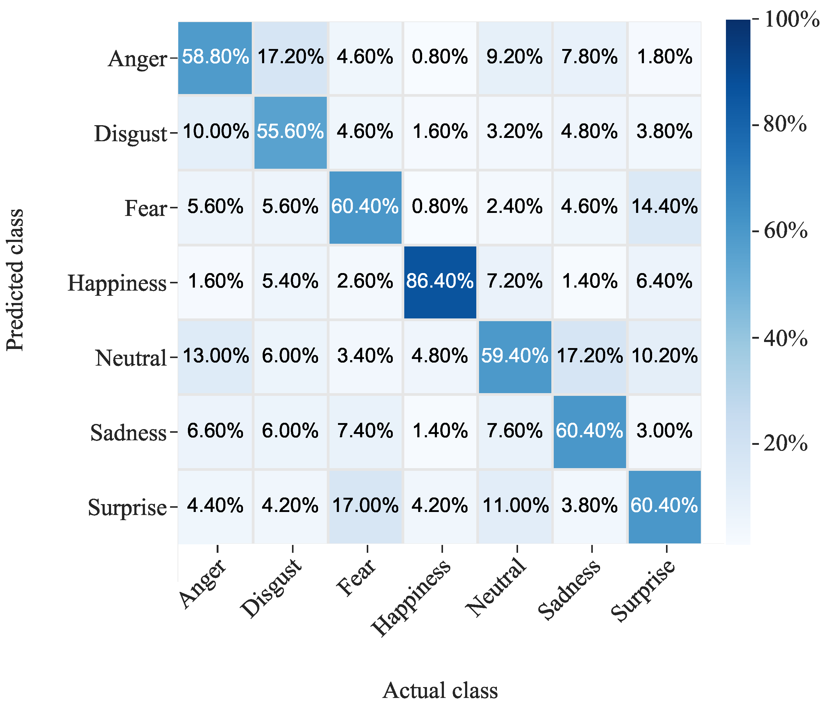
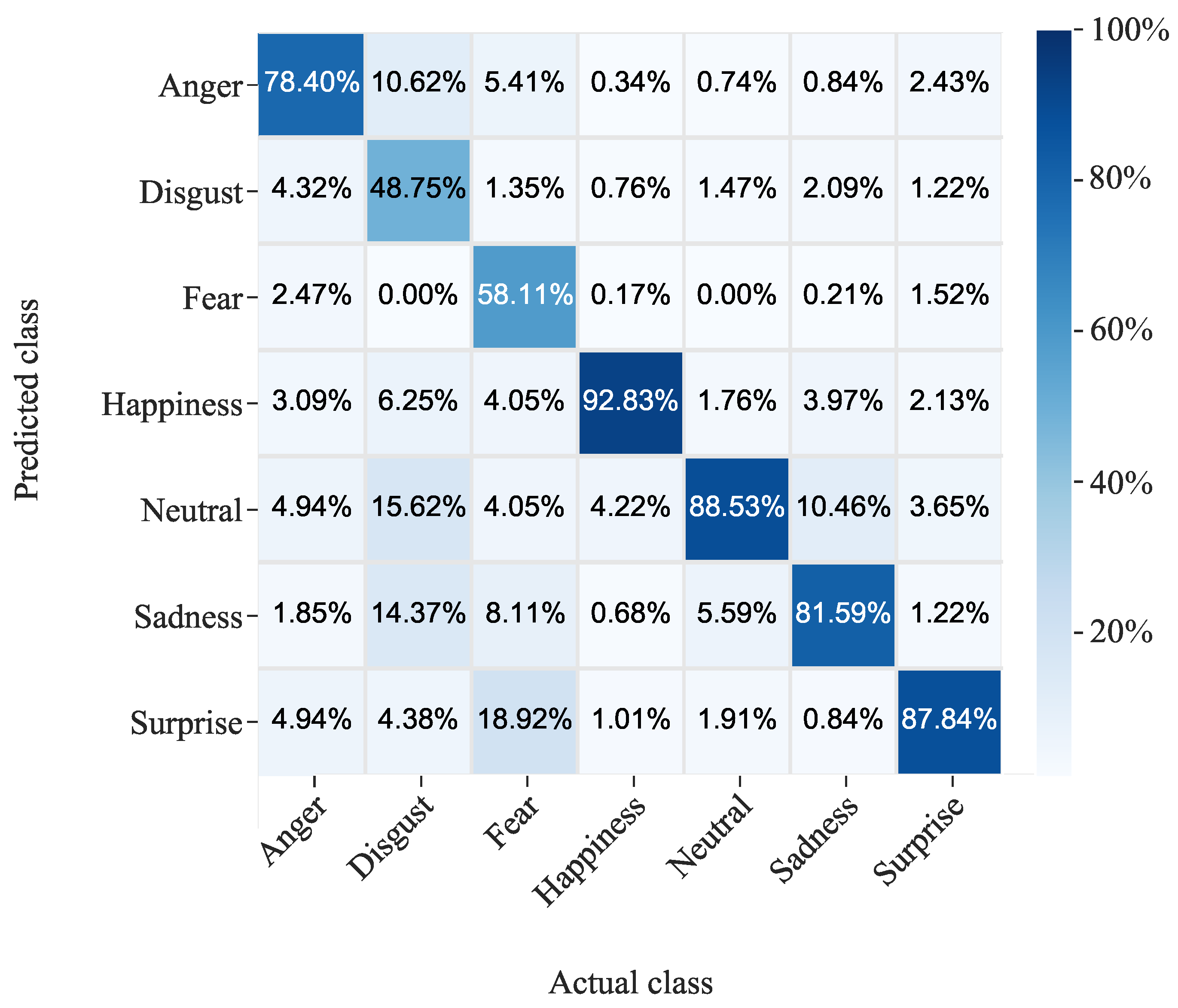
Figure 5 and
Figure 6 show the confusion matrices of our model evaluated on the test set of the above datasets.
In the AffectNet dataset, the best-classified emotion was happiness with an accuracy of 86.40%. The accuracy of the other classes ranged from 55.60% to 60.40%. As in the previous dataset, the class with the highest accuracy in RAF-DB was happiness, in this case with 92.93%. In this dataset, the three classes with the worst accuracy coincided with the three classes with the lowest number of images (see
Figure 4). This is probably because the RAF-DB dataset was not balanced during the training of the network, as was performed with AffectNet.
In both datasets, the worst-classified class was disgust, with 17.2% of the AffectNet images with this label being mistaken for anger and 10% of those with anger being assigned to disgust. The difficulty in recognizing disgust may be due to the fact that this facial emotion often shares visual features with other expressions, such as anger. In RAF-DB, on the other hand, there are not many false positives for disgust, but there are many false negatives; about 30% of the disgust images were assigned to neutral or sad. This pattern was also observed for fear, where the false positives did not exceed 5%, while the false negatives were more than 40%.
These results are consistent with those obtained in most of the works listed in
Table 4 and
Table 5, where happiness was always the best-classified emotion and disgust was usually the worst-classified. Considering that happiness is the easiest facial expression for humans to recognize, it is expected that images with this facial expression will be better labeled and, therefore, easier for the machine to recognize. When interpreting the data, it is important to note that the images in these datasets were obtained from Internet search engines, and it is not possible to know for certain what emotions the people in these images were experiencing. These datasets were labeled by human annotators, and there were discrepancies between the annotators’ responses for quite a few images, especially in the case of AffectNet, where the degree of inter-annotator agreement for eight facial expressions was 60.7%.
Next, we compared the best results obtained with several state-of-the-art methods on AffectNet and RAF-DB. For AffectNet with seven classes, we did not find any work using an image size like ours, so the comparison with other works is not entirely fair. As shown in
Table 4, a classification accuracy of 63.06% was obtained, which is 3.4% lower than the state-of-the-art, but higher than the accuracy obtained by some recent models using much larger images than ours.
On the other hand, for RAF-DB, the E-FCNN [
44] and RCAN [
43] methods were evaluated on images of a similar size to ours and reported similar results to those obtained with the proposed approach (see
Table 5). However, these two methods are based on super-resolution, which means that the neural networks were trained on images larger than those used for inference. In contrast, in the proposed method, the training images are the same size as the test images.
Regarding the number of trainable parameters, our model is one of the lightest with 11.17 million parameters, both for the baseline architecture and for the architectures where the splitting and voting strategy was implemented. Most of the papers listed in
Table 4 and
Table 5 did not report the number of trainable parameters or the GFLOPs of the model. Only a recent paper reported 35.74 million parameters and 3686 GFLOPs [
43]. However, considering only the network used as the backbone in each paper, it can be observed that most of the models used more trainable parameters than those used in our approach.
For example, some approaches [
19,
49,
58,
61] used VGG architectures for feature extraction with significantly more trainable parameters than the modified ResNet-18 we used. On the other hand, other works [
60,
63] used a ResNet-50 as their backbone, an architecture that has about 25 million trainable parameters in its usual implementation. The ResNet-18 architecture is one of the most-widely used [
49,
50,
51,
52,
53]. These approaches use this architecture as a feature extractor. ResNet-18 uses 11.69 million parameters in its usual implementation, but these papers used this architecture as a feature extractor and added other elements at the end of the network, so the total number of parameters of the complete model can be significantly higher.
5. Conclusions
In this paper, a residual voting network was proposed for the classification of low-resolution facial expression images. The introduction of the voting strategy into the network improved the accuracy of the baseline model without significantly increasing the number of trainable network parameters. Different intermediate points in the network at which images could be cropped were examined, and it was observed that the closer the point was to the input of the network, the greater the improvement in accuracy compared to the baseline architecture. However, the size of the forward pass also increased. Based on the above, the best point for cropping will depend on the application. It will be a matter of selecting the closest possible point to the network input, depending on the available computational resources.
In addition, the proposed method was compared with some of the more-recent approaches. The experimental results obtained showed that our method was able to achieve classification accuracies similar to those reported by other methods using images larger than ours. Therefore, we concluded that it is possible to use low-resolution images for training FER models without a significant reduction in classification accuracy.
The method presented in this paper, with slight modifications to adapt it to the output dimensions of the different layers of the network, can be applied to almost any CNN. Therefore, it will be necessary in the future to study the usefulness of this method in other network architectures and in other classification or even regression tasks.
A possible future research direction is to explore the feasibility of applying this method to networks operating at the standard 224 × 224 image size. Although the proposed method does not increase the number of trainable model parameters, it does increase the memory requirements. Investigating its performance on larger images could provide valuable information about its versatility and feasibility for other applications. Another promising research direction is the integration of this model into a ViT architecture. Both approaches share the partitioning of the image into multiple patches, suggesting that the creation of a hybrid model may be feasible.
Although the proposed model is intended for FER, it may also be interesting to explore whether it can improve the performance of the base model in other image-processing tasks. This research could help determine the true potential and usefulness of the model. In conclusion, the adaptability and performance of the proposed method gives rise to several avenues for future research.


 ,
, 


