1. Introduction
Reinforcement learning (RL) has recently gained notable attention in various fields, including autonomous driving, due to its capability to address unanticipated challenges in real-world scenarios. Autonomous driving software defects can pose potential risks, thus developing safe and efficient methods when using AI technologies for autonomous driving systems is important [
1]. Autonomous driving systems, by employing RL algorithms, are able to accrue experience and refine their decision-making procedures within dynamic environments [
2,
3,
4]. This can be largely attributed to RL’s inherent ability to adapt and learn from complex and fluctuating situations, demonstrating its aptitude for these applications. The basic concept of RL lies in the structure of Markov decision processes (MDP), a system where algorithms learn via a trial-and-error approach, striving to reach predetermined objectives by learning from mistakes and rewards. The aim of RL is to optimize future cumulative rewards and formulate the most efficient policy for distinct problems [
5]. Recent integration of deep learning with RL has demonstrated promising outcomes across various domains. This involves the employment of advanced neural networks such as convolutional neural networks (CNNs), multi-layer perceptrons, restricted Boltzmann machines, and recurrent neural networks [
6,
7]. By fusing reinforcement learning with deep learning, the system’s learning capabilities are significantly enhanced, allowing it to process complex data such as sensor feedback and environmental observations, thus facilitating more informed and effective driving decisions [
8]. However, the application of RL to autonomous driving presents a unique array of challenges, particularly when it comes to deploying RL in real-world environments. The uncertainties inherent in these environments can make the effective execution of RL quite challenging. As a result, researchers often struggle to achieve optimal RL performance directly within the actual driving context, highlighting the various obstacles encountered when applying RL to autonomous driving [
9]. Several challenges plague the application of RL to autonomous driving: overestimation phenomenon, learning time, and sparse reward problems [
10,
11].
Firstly, the overestimation phenomenon is prevalent in model-free RL methods, such as Q-learning [
12] and its variants like the double deep Q network (DDQN) [
13,
14] and dueling DQN [
15]. These methods are susceptible to overestimation and incorrect learning, primarily due to the combination of insufficiently flexible function approximation and the presence of noise, which lead to inaccuracies in action values. Secondly, the significant amount of learning time required is another hurdle. When RL is fused with neural networks, it generates policies directly from interactions with the environment, bypassing the need for a basic dynamics model. However, even simple tasks necessitate extensive trials and a massive number of data for learning. This makes high-performance RL both time-consuming and data-intensive [
16]. Lastly, the issue of sparse reward arises during RL training. This presents challenges in scenarios where not all conditions receive immediate compensation. Although techniques like hindsight experience replay (HER) [
17,
18] have been proposed to mitigate this issue, the direct application of RL to autonomous vehicles is still limited due to the complex fusion of information and potential system failures during the learning process. This paper addresses the challenges of RL in autonomous driving and reduces the reliance on extensive real-world learning by introducing a set of innovative techniques to enhance the efficiency and effectiveness of RL: data preprocessing through obstacle-dependent Gaussian (ODG) [
19,
20] DQN, prior knowledge through Guide ODG DQN, and meta-learning-based guided ODG DDQN.
The data preprocessing method employs the ODG algorithm to combat the overestimation phenomenon. By preprocessing distance information through ODG DQN, it allows for more accurate action values, fostering stable and efficient learning [
21]. The prior knowledge method draws on human learning mechanisms, incorporating knowledge derived from the ODG algorithm. This strategy mitigates the issue of sparse rewards and boosts the learning speed [
22], facilitating more effective convergence. Lastly, the meta-learning-based guide rollout method uses ODG DQN to address complex driving decisions and sparse rewards in real-world situations. By enriching prior knowledge using a rollout approach, this method aims to create efficient and successful autonomous driving policies.
Our main contributions can be summarized as follows:
Efficiency and speed of learning: The newly proposed RL algorithm utilizes ODG DQN on preprocessed information, enabling the agent to make optimal action choices, which significantly enhances the learning speed and efficiency.
Improvement of learning stability: With the use of prior knowledge, the guide-ODG-DQN helps mitigate the issue of sparse rewards, thus increasing the learning stability and overall efficiency.
Adaptability to various environments: The meta-learning-based ODG DDQN leverages model similarities and differences to increase learning efficiency. This allows for the reliable training of a universal model across diverse environments, with its performance demonstrated in environments like Gazebo and Real-Environment.
In this context, the purpose and objectives of this study are to propose a stable and efficient reinforcement learning method to effectively address the overestimation phenomenon, learning time, and sparse reward problems faced in the field of autonomous driving. By doing so, we aim to improve the performance of reinforcement learning, overcome the obstacles for implementing autonomous driving systems in real environments, and provide more stable and efficient vehicle control strategies.
The remainder of this paper is organized as follows: in the stable and efficient method section, we mainly introduce the proposed reinforcement learning algorithm. To verify the effectiveness of our work, the experimental evaluations and necessary analysis are presented in the experiment. Finally, we summarize our work in the Conclusions section.
2. Stable and Efficient Reinforcement Learning Method
LiDAR (light detection and ranging) information serves as an invaluable perspective for autonomous driving systems, functioning much like a driver’s sense by identifying obstacles through environmental analysis. LiDAR-based RL methods have found extensive application in research focused on judgement and control within autonomous driving systems such as the partially observable Markov decision process (POMDP) [
23]. However, learning methodologies based on Q-learning, such as DDQN, encounter persistent overestimation issues, posing obstacles to the enhancement of learning efficiency and convergence speed.
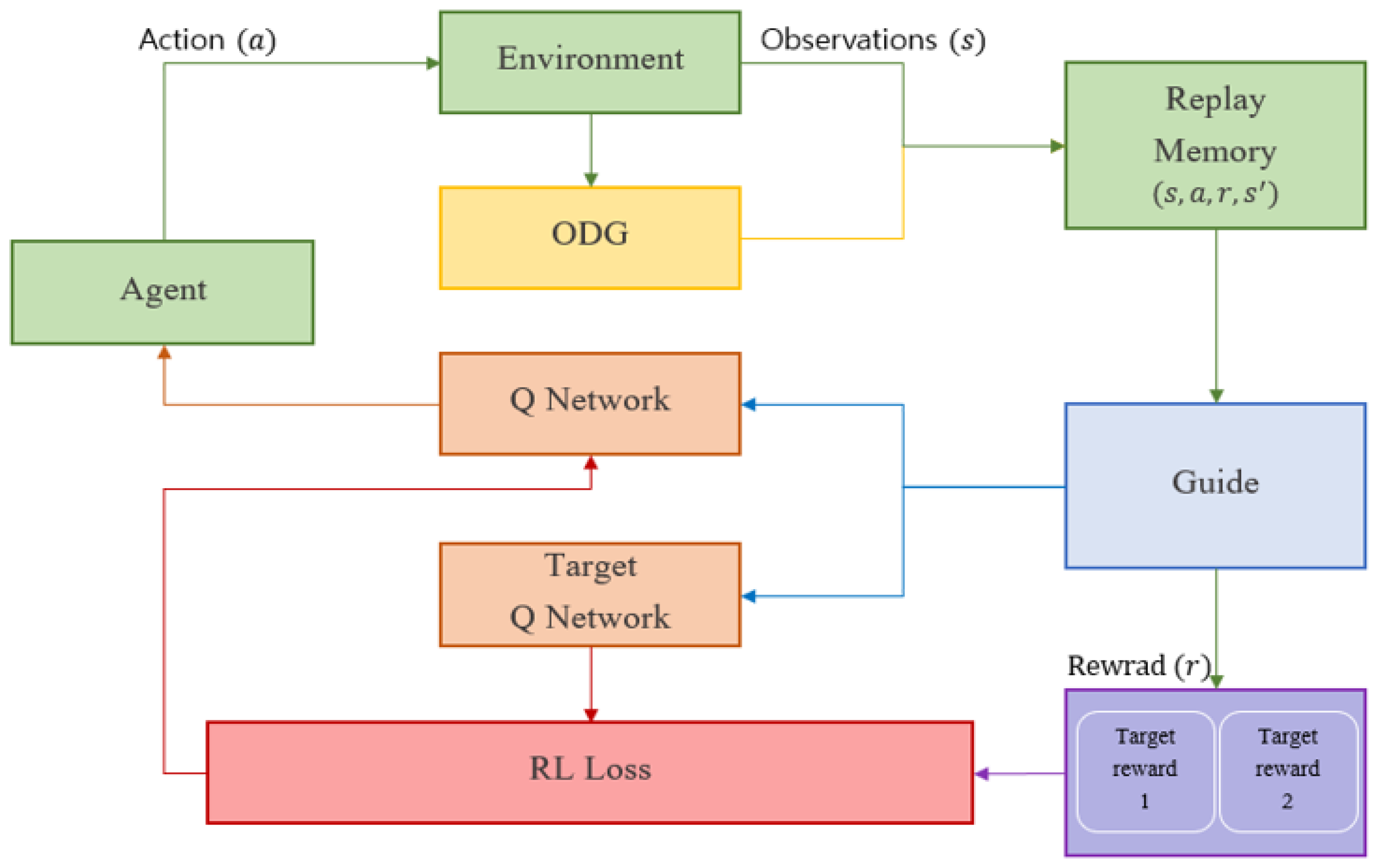
To mitigate these issues, we propose a method that preprocesses and transforms the LiDAR value into valuable information attuned to the operating environment, implementing it as the ODG technique [
24]. This approach, as depicted by the ODG module (in yellow) of
Figure 1, is designed to reduce learning convergence time and boost efficiency by preprocessing RL input data, thus remedying scenarios with inaccurate action values. Furthermore, we introduce the concept of prior knowledge to address the sparse rewards issue that impedes RL’s learning stability [
25]. By integrating prior knowledge information from sparse reward sections, as demonstrated in the guide-ODG-DQN framework shown in the guide module (in blue) of
Figure 1, we can enhance learning stability.
It is noted that in RL, model performance can decline when the learning environment changes. Thus, we propose the meta-Guide ODG-DDQN method, represented in the target reward module (in purple) in
Figure 1, to devise a more robust and adaptable RL algorithm. After training the model according to an initial goal, we modify the reward function to attain subsequent objectives. This approach effectively communicates the action value to the agent in diverse obstacle environments with reliability and swiftness. The proposed methodology consists of three progressively developed algorithms.
2.1. ODG DQN
Overestimation, a consequence of inaccurate action values, is underscored as a critical issue in the DDQN literature [
13,
26,
27,
28]. Traditional LiDAR information incorporates an infinite range, which represents all information at the maximum distance or the value of obstacle-free spaces. This arrangement leads to an overlap of LiDAR information within the system, causing overestimation and impeding the model’s ability to select these infinite values. In Q-learning, this predicament can be defined by
for a given state
s, as detailed in Equation (
1). When environmental noise triggers an error, it is defined per Equation (
2). If the max function is applied at the moment of peak value in Q-learning for action selection, the expression aligns with Equation (
3). The bias, symbolized by
, causes the model to overestimate the bias relative to the optimal value with Q-learning [
12,
13].
where
m is the number of actions and
C is a constant.
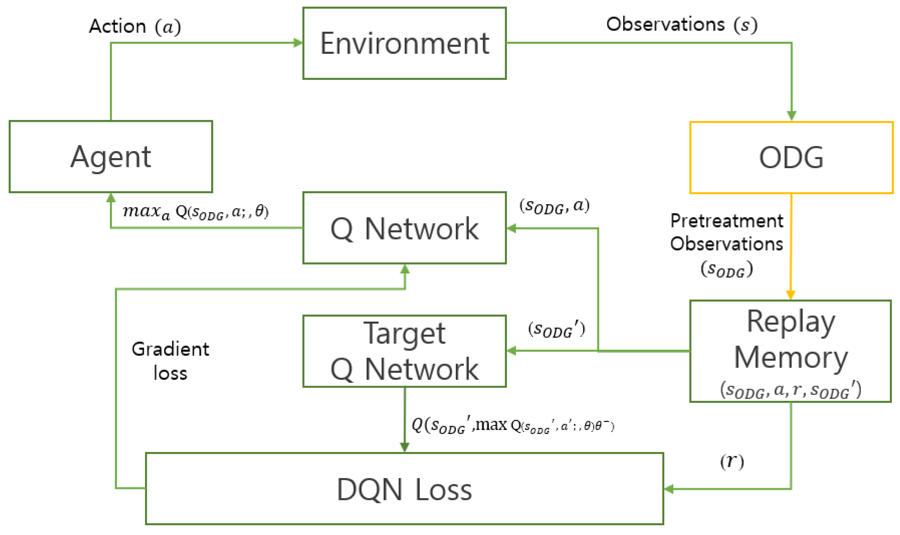
To address this overestimation, our algorithm utilizes the ODG module to preprocess state values. Illustrated in
Figure 2, this module, based on Equation (
4) with DQN [
6], is engineered to establish an optimized steering angle model for the agent via Q-learning-based RL. This paves the way for the development of an optimized path plan built on the steering angle generated by the agent.
LiDAR information, a principal component in autonomous driving systems, is preprocessed via the ODG module, subsequently offering the processed data to the RL approach as the state value. Through the use of a Gaussian distribution, the ODG module converts LiDAR information into continuous values. As depicted in
Figure 3, the creation of a unique state happens when an agent selects an action, preventing the duplication of action values and facilitating a more efficient selection of the optimal action value in accordance with the equation.
For the implementation of our proposed algorithm to RL using LiDAR information, a standard procedure in autonomous vehicles, we employ ODG-based preprocessed LiDAR information. As demonstrated in
Figure 4, the yellow line corresponds to the original LiDAR data, whereas the blue line symbolizes post-processed data. These data include information on obstacle location and size, derived using Equation (
5) with ODG [
19].
where
In contrast to the overlapping LiDAR information provided by conventional methods, ODG supplies non-overlapping LiDAR data, adjusting the maximum range according to the obstacle’s size and distance. This preprocessing enables the agent to make more efficient decisions related to optimal action values based on the processed information, thereby enhancing both the speed and efficiency of learning. The reward function used for training is defined in Equation (
8).
where
represents the target reward,
denotes the reward for speed, and
signifies the reward for steering angle.
2.2. Guide ODG DQN
The soft actor critic (SAC) method [
29] is a robust approach that allows for the observation of multiple optimal values while avoiding the selection of impractical paths. This facilitates a more extensive policy exploration. The SAC employs an efficient and stable entropy framework for the continuous state and action space. As delineated in Equation (
10) with SAC [
29], the SAC learns the optimal Q function through updating Q-learning via the maximum entropy RL method.
The algorithm initially makes the guide value sparse and, as learning progresses, gradually densifies it, employing the gamma value as outlined in Equation (
12) with SAC [
29]. The term min A is representative of the environmental vehicle.
A report on hierarchical deep RL, an approach that implements RL via multiple objectives, emphasized the need to solve sparse reward problems as environments become increasingly diverse and complex. Normally, in problems tackled by RL, rewards are generated for each state, like survival time or score. Every state is linked to an action, receives a reward, and identifies the Q-value so as to maximize the sum of the rewards. However, there are instances where a reward may not be received for each state. These scenarios are referred to as sparse rewards.
where
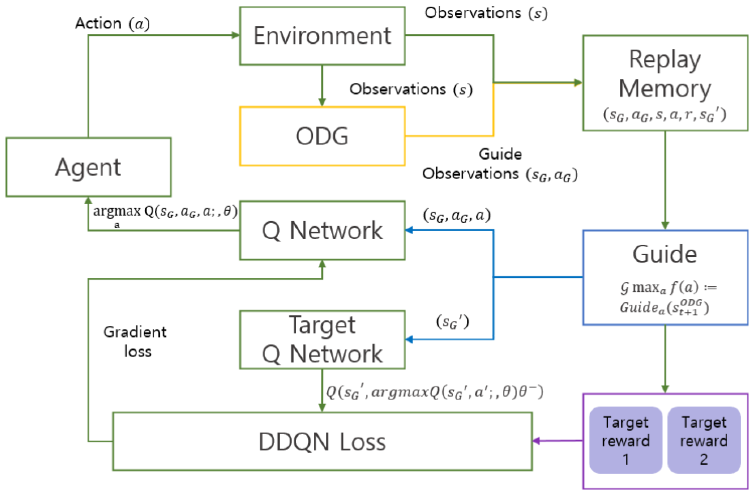
Our proposed solution to these issues is the guide-ODG-DNQ model that integrates SAC with ODG-DQN. This proposed guide-ODG-DQN algorithm transforms the initial Q-value from the state value. This value is extracted from the environment, and it is connected with the ODG formula, which is our prior knowledge, and the LiDAR value extracted with ODG, as depicted in
Figure 5. The algorithm extracts a guide action that minimizes the cases where a reward is not received for every state.
The guide-ODG-DQN is designed to store high-quality information values in the replay memory from the outset based on prior knowledge. The agent then continues learning based on this prior knowledge, facilitating easier adaptation to various environments and enabling faster and more stable convergence. Moreover, to prevent over-reliance on prior knowledge that could compromise the effectiveness of RL, the agent learns from its own experiences during the learning process, which are represented by the gamma value. The agent also contrasts this newly learned information with the values derived from the existing prior knowledge. Consequently, our proposed guide-ODG-DQN mitigates the sparse reward phenomenon, thereby enhancing both the stability and efficiency of the learning process.
2.3. Meta-Learning-Based Guide ODG DDQN
RL is fundamentally a process of learning through trial and error. The RL agent must experience a diverse set of situations, making decisions in each scenario to understand which actions yield the highest rewards. Striking a balance between experimentation, to ensure no high-reward actions are overlooked, and leveraging acquired knowledge to maximize rewards is crucial. However, achieving this balance typically necessitates numerous trials and, consequently, large volumes of data. Training an RL agent with excessive data might result in overfitting, wherein the agent conforms too closely to the training data and fails to generalize well to new circumstances.
To overcome these limitations, we introduce a novel method known as meta-learning-based guide-ODG-DDQN. This approach involves storing rewards for each step an integral part of RL in the replay memory, with the stored rewards divided according to the number of targets to be learned as shown in
Figure 6. This model facilitates few-shot learning within RL by training the model to recognize similarities and differences, thus preparing it to perform proficiently in unfamiliar environments with minimal data. The training is guided by two main objectives. The first is to train the target model using the initial reward, while the second is to continue learning by reducing the weight assigned to the initial reward and increasing the weight of the reward for the subsequent target, as depicted in Equation (
15).
By applying our meta-learning-based ODG RL, the model achieves multiple significant outcomes. It allows for the training of a universal model that can operate reliably across various environments. The model’s efficiency of learning is boosted due to its ability to identify similarities and differences. Furthermore, learning can proceed using a common target while preserving the existing target. In essence, the proposed algorithms augment the efficiency and stability of traditional RL methods, safely accelerating the learning speed within a virtual environment, which ultimately improves efficiency when the model is implemented in real-world environments.
3. Experiment
In the process of validating our proposed algorithm, we conducted an experiment evaluating key aspects such as learning efficiency, stability, strength, and adaptability to complex environments. Learning efficiency was determined by examining the highest reward achieved as learning started to converge, in relation to the number of frames experienced in the virtual environment. The DQN algorithm was used as the basis to analyze the rate of convergence and the magnitude of the reward. For the evaluation of learning stability, we assessed the consistency between the path plan generated through RL
and the target path produced by ODG
. Here,
represents the set of paths. This assessment involved the use of the root mean square error (RMSE), where
and
represent the path plans formed through RL and ODG, respectively. The route yielding the highest reward was considered optimal. Finally, we evaluated the algorithm’s performance in complex environments. This part of the evaluation was focused on the vehicle’s ability to effectively navigate through real world maps, leveraging learning strength. We also tested the resilience and adaptability of the algorithm when faced with unfamiliar scenarios without further training. Metrics such as entry and exit speed, as well as racing track lap time, were used to measure performance. The evaluation environments were chosen with care for distinct aspects of the study: the Gazebo map was used to evaluate learning efficiency and stability, the Sochi map for learning strength, and the Silverstone map to test adaptability to complex conditions, as shown in
Figure 7. The experiment setup was designed to reflect real world dimensions, such that each unit length in the simulation corresponded to one meter in reality [
30,
31].
First, the index for learning efficiency is determined as follows. As learning begins to converge, the learning efficiency corresponding to the highest reward for the number of frames (in millions) experienced in the virtual environment is considered. Based on the DQN algorithm, we evaluate how fast convergence occurs and how high the reward is.
Second, the evaluation metric for learning stability assesses how well the path plan generated through RL matches the target path pursued. The path plan created by RL in the virtual environment,
, and the path plan created with the ODG,
, are represented in terms of the
. Both
and
are individually compared with the reference path, and their respective errors are calculated using Equation (
16).
where
represents the path generated by ODG in
, which is known to exhibit high real-time performance and stability, and
corresponds to
, which is the path plan generated through RL. The optimal route with the highest reward is considered.
n is the number of steps the agent operates in the simulation environment, corresponding to the episodic steps in RL. A smaller
corresponds to a more stable.
Finally, we evaluate the performance in complex environments, as depicted in
Figure 7. The assessment metrics focus on how effectively the vehicle navigates through intricate obstacles while ensuring safety and speed. We showcase the learning strength in the Sochi Circuit and the learning diversity in the Silverstone Circuit. For this evaluation, we utilized real maps and employed the metrics of “Enter and Exit Speed” and “Racing Track Lap Time” to assess the agent’s performance. In summary, our results demonstrate the learning strength and diversity of the proposed algorithm in handling complex environments and showcase its robustness when encountering new scenarios without further training.
3.1. Learning Performance and Efficiency Evaluation
The hyperparameters used in set up are listed in
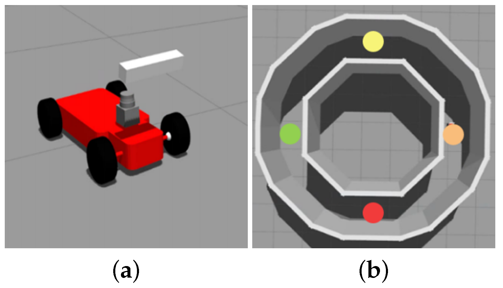
Table 1. The set up is aimed at verifying the efficiency of the algorithm to be applied in a real environment. Therefore, reducing the learning time is the priority. To evaluate whether learning efficiency and stability are ensure, a basic circular map is selected, and a performance comparison experiment is conducted for each RL algorithm: DQN, ODG-DQN, DDQN, and guide-ODG-DQN. The agent model and environment used in the experiment are shown in
Figure 8.
The reward function used for training is defined in
Table 1. First, to compare the DQN and ODG-DQN algorithms for the Gazebo map, we determine the number of steps in which the checkpoint is reached during training, as indicated in
Table 2. In DQN, over 50% of untrained failure cases are overestimated, whereas in ODG-DQN, 10% of untrained failure cases occur, corresponding to overestimation occurrence reduced by 80%.
Guide-ODG-DQN and DDQN are compared under the same conditions.
Figure 9a shows the results of learning in terms of the epoch values of the safe convergence section for each algorithm implemented 10 times. As indicated in
Table 3, the learning convergence rate increases by 51.7%, 89%, and 16.8%, respectively, compared with the other algorithm.
Figure 9b shows that the learning is inappropriate due to overestimation in the case of DQN. In the cases of ODG-DQN, DDQN, and guide-ODG-DQN, learning converges at approximately 500, 300, and 200 epochs, respectively the results are summarized in
Table 4.
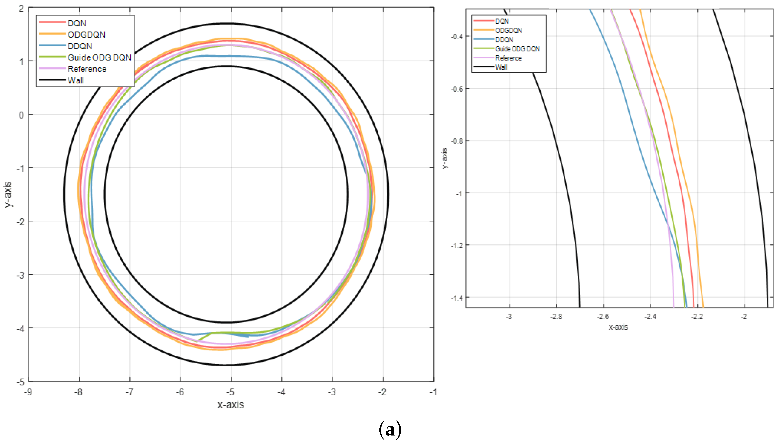
Next, to evaluate the stability of the RL results, the center line corresponding to the Gazebo map is applied as a reference. The path generated by each algorithm is shown in
Figure 9a. Moreover,
Table 5 shows the results obtained by comparing the algorithms in terms of the RMSE, as defined in Equation (
16). The RMSE for guide-ODG-DQN is 0.04, corresponding to the highest stability. The guide-ODG-DQN achieves the lowest RMSE, corresponding to the highest stability, as shown in
Figure 9c.
3.2. Results through Simulation That Mimics the Real Environment
The hyperparameters values used in circuit are listed in
Table 6. As the evaluation metric for a complex environment, shown in
Figure 10a, the method of learning the speed is considered instead of that for learning angles. Therefore, the angle is set to that associated with the ODG to ensure stability. The reward function used for all RL frameworks is the same as that defined in
Table 6.
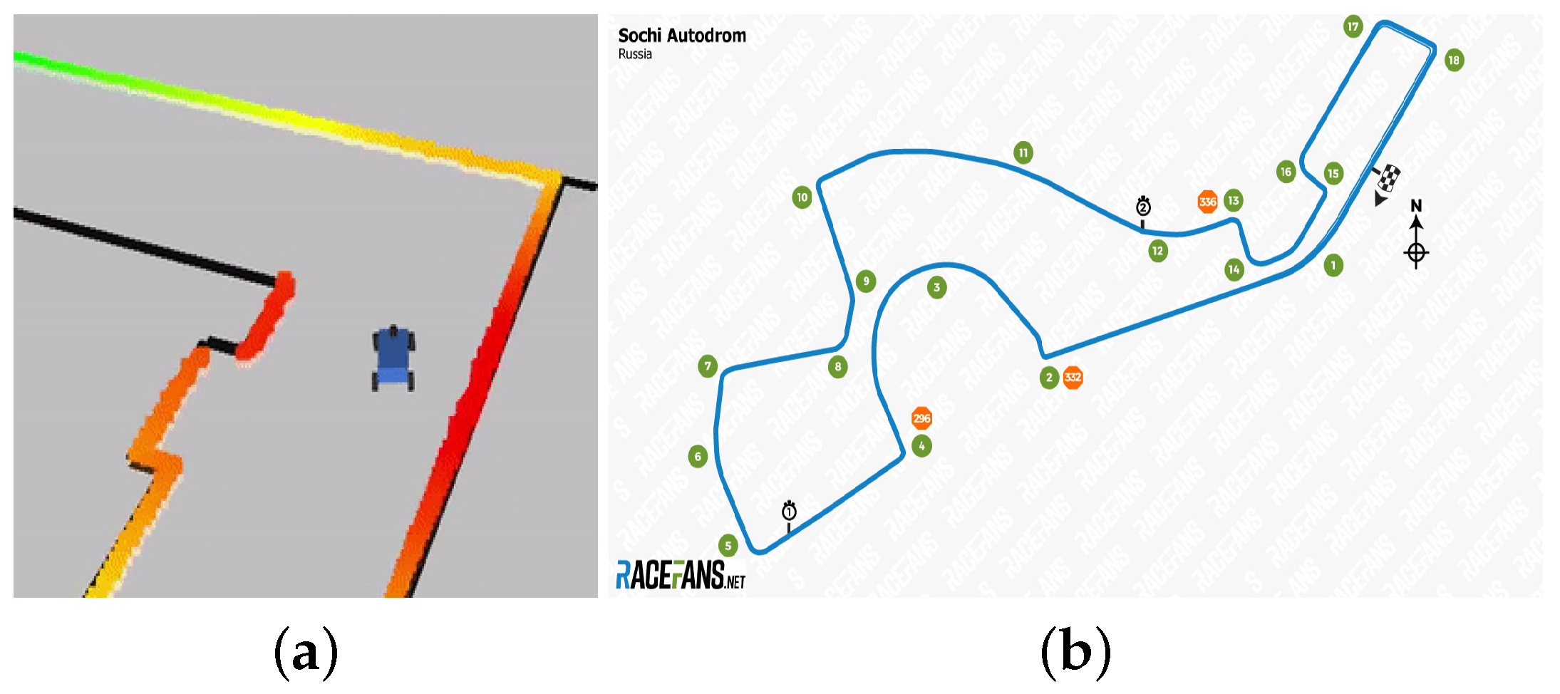
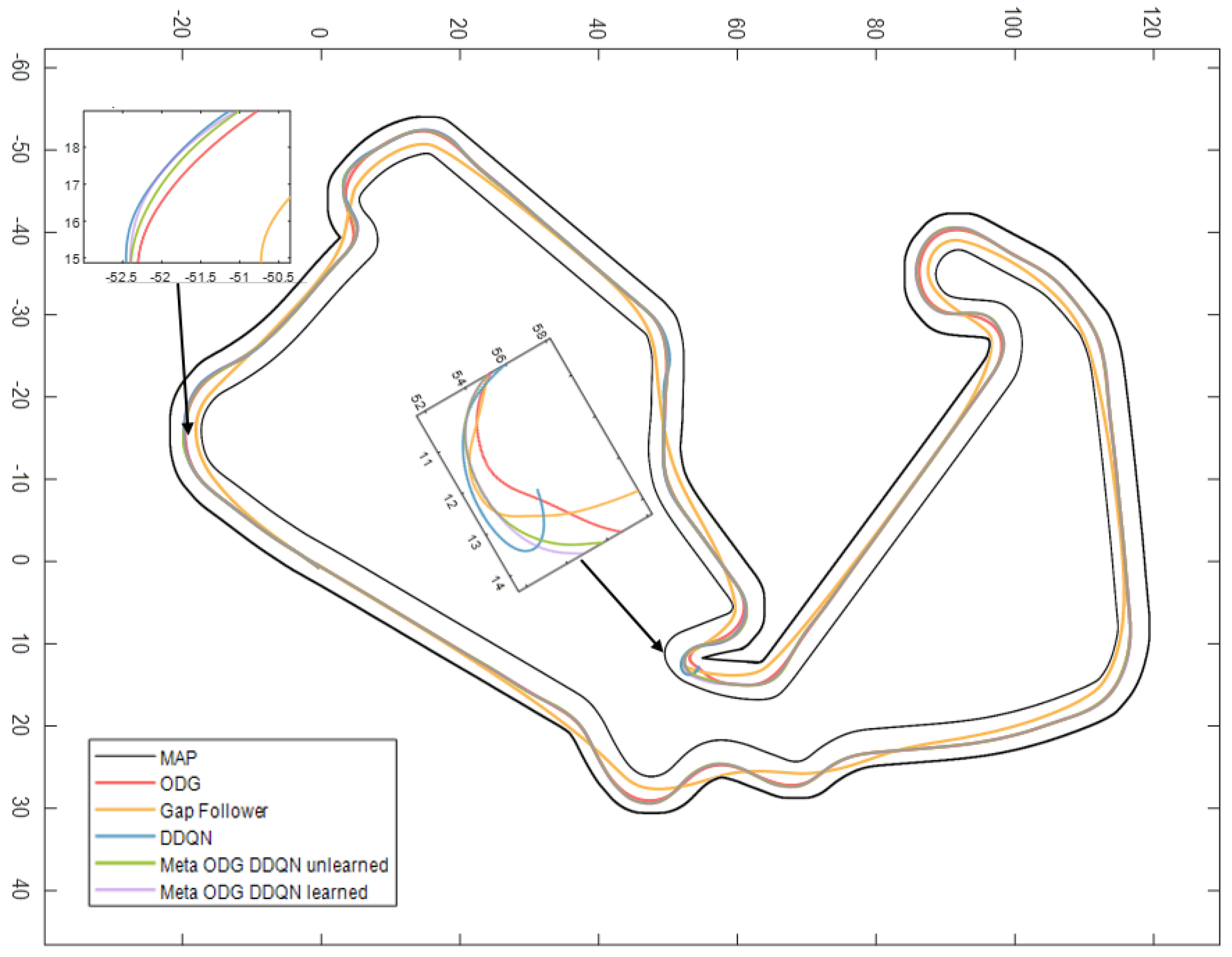
Figure 10b shows the official competition map provided by F1TENTH. Using the control point specified in the actual Sochi Autodrom map, we compare the path in the winding road and hairpin curve.
The agent starts at the wall of control point 1. Linear velocity graphs for ODG, Gap Follower, DDQN, and meta ODG DDQN are shown in Figure 13. In this case, 100 points on the x-axis are used as control points, and 100-step linear velocity values are output on both sides based on these values.
3.2.1. Sochi International Street Circuit
The Sochi Autodrom, previously known as the Sochi International Street Circuit and the Sochi Olympic Park Circuit, is a 5.848 km permanent race track in the settlement of Sirius next to the Black Sea resort town of Sochi in Krasnodar Krai, Russia, as shown in
Figure 11. Here, the learning strength is demonstrated, in the Sochi Circuit.
Table 7 lists the average speed for each control point for each algorithm.
Table 7 shows that the ODG algorithm that prioritizes stability achieves the lowest value of 7.66, and the meta ODG DDQN achieves the highest value of 8.58. In other words, the meta ODG DDQN completes the Sochi Autodrom with a speed 12.01% higher than that of the ODG.
As shown in
Figure 12a, to examine the speeds of entry and exit at the control point, which are of significance in a racing game, the entry and exit speed for each algorithm are presented in
Table 8. In the case of ODG, which is an algorithm that prioritizes stability, as shown in
Figure 12b, understeer or oversteer does not occur [
32,
33]. A report on racing high-performance tires [
34] indicates that in this driving method, the vehicle enters at a high speed and exits at a low speed.
As shown in
Table 9, ODG selects a drive with a 13.9% speed reduction. The racing algorithm, Gap Follower, uses an out-in-out driving method with a 3.41% deceleration. However, the DDQN and meta ODG DDQN algorithms lead to oversteer to achieve maximum speed based on the angle extracted from the ODG, which pursues stability, causing the vehicle to spin inward compared to the expected route. So, DDQN and meta ODG DDQN show a driving method without deceleration at control points of 1.33% and 0.46%, respectively, by drawing a path.
Moreover, the lap time is compared for the map shown in
Figure 10b by considering two laps (based on the F1TENTH formula).
Table 10 indicates that meta ODG DDQN achieves the highest speed.
Linear velocity graphs for ODG, Gap Follower, DDQN, and meta ODG DDQN are shown in
Figure 13; using the control point specified in the actual Sochi Circuit, we compare the path in the winding road and hairpin curve, as shown in
Figure 14.
3.2.2. Silverstone Circuit
Silverstone Circuit is a motor racing circuit in England, near the Northamptonshire villages of Towcester, Silverstone, and Whittlebury, as shown in
Figure 11. In this result, the learning diversity in the Silverstone Circuit is demonstrated.
Using the RL model trained in Map Sochi, we conduct an experiment to determine the degree of robustness to unfamiliar and complex environments. Therefore, we use the algorithms ODG, Gap Follower, DDQN, and meta ODG DDQN. In addition, the meta ODG DDQN algorithm is trained in a new environment. In other words, the robustness of the new environment (c) was compared based on the driving style learned in (b) shown in
Figure 7.
Table 11 presents the results for a new environment. DDQN fails; however, meta ODG DDQN exhibits high performance with the lowest lap time, as shown in
Figure 15. In this result, the learning diversity in the Silverstone Circuit is demonstrated.
4. Conclusions
This paper introduces a novel RL-based autonomous driving system technology that implements ODG, SAC, and meta-learning algorithms. In autonomous driving technology, perception, decision-making, and control processes intertwine and interact. This work addresses the issues of the overestimation phenomenon and sparse rewards problems by applying the concept of prior knowledge. Furthermore, the fusion of meta-learning-based RL yields robust results in previously untrained environments.
The proposed algorithm was tested on official F1 circuits, a racing simulation with complex dynamics. The results of these simulations emphasize the exceptional performance of our method, which exhibits a learning speed up to 89% faster than existing algorithms in these environments. Within the racing context, the disparity between entry and exit speeds is a mere 0.46%, indicating the smallest reduction ratio. Moreover, the average driving speed was found to be up to 12.01% higher.
The primary contributions of this paper comprise a unique combination addressing the challenges of overestimation phenomenon and sparse rewards problems effectively in RL. Another major contribution is the demonstrated robust performance of the integrated meta-learning-based RL in previously untrained environments, thereby showcasing its adaptability and stability. Furthermore, we validated the performance of our proposed method via complex racing simulations, particularly on official F1 circuits. The results highlighted its superior performance in terms of learning efficiency, speed, stability, and adaptability.
In essence, this paper tackles the significant challenges encountered during the reinforcement learning process by introducing an algorithm that bolsters the efficiency and stability of RL. The high-fidelity simulations used in this study offer a realistic testing environment closely mirroring real-world conditions. Given these advancements, our proposed algorithm demonstrates significant potential for real-world applications, particularly in autonomous vehicles where learning efficiency and operational stability are of the utmost importance.
As for future research, we suggest adding various multi-tasks to verify stable and efficient learning in more complex environments. Based on this, we aim to study efficient RLs in real environments through meta-learning, with as few iterations as possible.


 ,
, 


