Article

A Two-Stage Image Inpainting Technique for Old Photographs Based on Transfer Learning

1
School of Automation and Information Engineering, Sichuan University of Science & Engineering, Yibin 644002, China
2
Artificial Intelligence Key Laboratory of Sichuan Province, Sichuan University of Science & Engineering, Yibin 644002, China
3
Sinograin Chengdu Grain Reserve, Chengdu 610000, China
*
Authors to whom correspondence should be addressed.
Electronics 2023, 12(15), 3221; https://doi.org/10.3390/electronics12153221
Submission received: 4 July 2023 / Revised: 22 July 2023 / Accepted: 24 July 2023 / Published: 25 July 2023

Abstract

:
To address the challenge of sparse old photo datasets, we apply transfer learning to image inpainting tasks. Specifically, we improve a two-stage image inpainting network that focuses on collaborative subtasks. We also design a transform module based on the cross-aggregation of windows to improve long-distance contextual information acquisition in image inpainting and enhance the integrity of images in terms of structure and texture. Our improved two-stage network has a significantly better repair performance compared to that of the current common inpainting methods. We further apply transfer learning techniques by utilizing the improved two-stage image inpainting network as the base network and decoupling the generator into a feature extractor and classifier, which consist of an encoder and a decoder, respectively. We obtain a domain-invariant feature extractor through minimax game training using source and target domain data. This feature extractor can be combined with the original encoder to restore old photo images. To verify the effectiveness of our approach, we conducted comparative experiments. Our results show that the PSNR, SSIM, and FID indexes of the model using transfer learning are 11.8%, 2.96%, and 44.4% higher than those without transfer learning, respectively. These findings suggest that applying transfer learning techniques can be an effective solution to address the challenge of sparse old photo datasets in image inpainting tasks.

1. Introduction

Photographs serve as important records of specific times and are a crucial tool for documenting historical development and family changes in modern times. However, early paper photographs were prone to damage due to the use of poor technology and preservation practices. To address the challenges of preserving paper photographs, digital image inpainting technology can be used to restore old and damaged photographs to their original appearance as much as possible [1,2]. Traditional image inpainting algorithms mainly include partial differential algorithms [3,4,5] and texture synthesis algorithms [6,7], which have obvious limitations due to the use of only the peripheral information surviving in the original image. When repairing complex and non-repetitive structures, these algorithms may produce unsatisfactory results.
In recent years, there has been significant progress in the use of deep learning techniques in computer vision and image processing, and the use of large numbers of images to train networks has enabled trained models to have a significant amount of prior knowledge, providing a new approach to image inpainting [8]. In particular, Generative Adversarial Networks [9] have been proposed and achieved promising results in image inpainting tasks [10]. Pathak et al. [11] designed and applied GANs based on traditional Convolutional Neural Networks and proposed Context Encoders to send the output of the network to a discriminator to detect the truth, which greatly improved the plausibility of the results. However, the performance of neural networks typically depends on a large amount of training data, which makes them unsuitable for areas with minimal training data, changing scenarios, and changing tasks. To address the challenge posed by sparse samples of old photos, this paper introduces transfer learning to transfer the trained model on open-source datasets to the small dataset collected by us, so that the final model can have a generalization performance using standard datasets. Specifically, the portability of deep features [12] is used to map images with intermediate- or high-level features using pre-trained models and train target-specific classifiers from them [13], which is a process commonly referred to as feature selection. Fine-tuning the source model for the target data is also feasible, and it usually is more effective as it optimizes the entire network for the target task. Therefore, fine tuning has become the rule of thumb for deep transfer learning with limited domain data [14,15]. During the fine-tuning process, the source model needs to be moderately tuned to avoid overfitting, as deep networks are over-parameterized for small-scale target tasks. Unlike traditional machine learning and deep learning, which require labeled data for model training, transfer learning can use previously accumulated knowledge to discover commonalities in problems and apply generic knowledge learned in certain tasks to similar tasks, enabling the model to learn in a more generalized manner.
As there have been only a few studies on the application of transfer learning in the field of image inpainting, this paper aims to address this gap by introducing transfer learning into the two-stage inpainting network for training. Due to the limited number of self-collected old photo data samples, overfitting and other issues are likely to occur during the training of deep neural networks. Therefore, this paper proposes a transfer learning-based approach for inpainting damaged old photos, which allows the effective training of a better model using only a small number of old photo samples. The main contributions of this paper are as follows:
  • In this paper, a two-stage image inpainting network is constructed, which embeds images into two collaborative subtasks, which are structure generation and texture synthesis under structure constraints, and embeds the window cross aggregation-based transform module into the generator, which can effectively acquire the image long-range dependencies, thereby solving the problem that convolutional operations are limited to local feature extraction and enhancing the long-range contextual information acquisition capability of the model in image inpainting.
  • Transfer learning is applied to image inpainting technology. The improved two-stage image inpainting network in this paper is used as the basic network, and the generator is decoupled into a feature extractor and classifier, which are an encoder and a decoder, respectively. A domain-invariant feature extractor is obtained through the training of the minimax game using source domain data and target domain data. The feature extractor can be combined with the original encoder to repair the old photo image, and the restoration of small sample old photo image dataset is realized.
  • The experiments demonstrate that the two-stage network constructed in this paper has a better inpainting performance, and the inpainting of old photos using the transfer learning technique is better than that without the use of transfer learning, which proves the effectiveness of the method.

2. Related Work

2.1. Image Inpainting Technique

Deep learning’s ability to map deep features perfectly fits the requirements of image inpainting and shows the direction for new image inpainting methods. Recently, Nazeri et al. [16] proposed a two-stage GAN model named “EC”. The model combines the two stages of edge information prediction and image inpainting. It first generates the edge map of the missing region, and then sends it into the inpainting network as the guiding information for image inpainting, obtaining a relatively good restoration effect. Xiong et al. [17] demonstrated a similar model that, unlike EC, uses foreground object contours as a structural prior instead of edges for information. Ren et al. [18] pointed out that edge-preserving, smoothed images provide a better global structure due to them capturing more semantics, but these methods require a higher accuracy for structures, for instance, edges and contours. Some researchers have utilized the correlation between texture and structure to solve this problem. Li et al. [19] designed a progressive visual structure reconstruction network to progressively reconstruct structures and their associated visual features. They entangle the reconstruction of visual structures and visual features to benefit each other by sharing the parameters. Yang et al. [20] introduced a multitasking framework to generate sharp edges by adding structural constraints. Liu et al. [21] proposed a mutual coding decoding to simultaneously learn about convolutional features that correspond to different layers of structure and texture. However, a single shared framework is difficult for modeling textures and structures. Therefore, in order to effectively realize the restoration of image structure and texture information, Guo [22] et al. divided image inpainting into two subtasks, texture synthesis and structure reconstruction. They proposed a new dual-stream network for image inpainting to further improve the performance of image inpainting. Since existing image inpainting techniques are outputting only one restoration result for a broken image, but the nature of image inpainting is an uncertain task, and its output should not be limited. Based on this idea, Liu [23] et al. proposed a probabilistic diverse GAN algorithm. The closer to the center of the image hole that the area studied is, the higher its diversity is, and the more diverse it is, and thus, good results are obtained.

2.2. Transfer Learning Method

Deep learning-based transfer learning methods, that is, deep transfer learning aiming to reduce the time and cost of the training process, have become a popular research direction at present. In some domains (e.g., medical images, etc.) [24], there is the problem of difficulty in obtaining large datasets. Transfer learning provides a better solution for these domains. In addition, pre-trained models for specific jobs can be applied on simple edge devices with a limited processing power and training time, and the development of deep transfer learning opens the door to more intuitive and sophisticated artificial intelligence. Ge et al. [25] developed a method for fine-tuning by using additional data obtained from a large-scale dataset. Cui et al. [26] successfully applied the knowledge learned from large-scale datasets to domain-specific small-scale data through fine-tuning and won first place in the 2017 iNaturalist large-scale species classification challenge. As a result, their research provides new ideas for subsequent deep transfer learning. For example, Long et al. [27] proposed a new Deep Adaptation Network based on this, which generalizes deep Convolutional Neural Networks to new domain-adapted scenarios where Deep Adaptation Networks can learn transferable features with statistical guarantees and scale linearly using the unbiased estimation of kernel embeddings. Tzeng et al. [28] developed a method based on using GANs to train encoders for target samples. They use an adaptation layer to compute the Maximum Mean Difference between the source and target domain features [29]. Haeusser et al. [30] proposed the utilization of the association between source and target features in the training process. They aim to maximize the invariance of the learned feature domain, while minimizing the error in the source samples. In the field of image inpainting, the combination of deep neural networks and transfer learning technology has been successfully carried out in a preliminary exploration and has been applied to the image inpainting problem under the condition of large mask areas. Chen et al. [31] designed a transfer learning network that, for the first time, accomplished large mask image inpainting guided by a high-level understanding of abstract neuronal representation images. Zhao et al. [32] proposed a small-sample unsupervised joint transfer learning approach that combines fine-tuning with direct transfer training to enable the network to learn knowledge about the target domain.

3. Two-Stage Image Inpainting of Old Photos Based on Transfer Learning

The two-stage image inpainting network constructed in this paper adopts the BIFPN feature fusion network proposed by Li et al. [33], which effectively strengthens the fusion and interaction of information. The original network generator is a two-stream generator. In this paper, a two-stage network is adopted. By embedding the transform module into the generator network in the form of residuals, the distant image dependence relationship can be effectively obtained. This solves the problem that convolution operation is limited to local feature extraction and enhances the model’s capability to obtain long-distance contextual information in image restoration. The repair performance of the network has been improved. By applying transfer learning to train the image inpainting network, the large public dataset, CelebA, is used as the source domain, and old photo images are used as the target domain. A domain-invariant feature extractor is obtained, which can cope well with the restoration task of old photo images.

3.1. Two-Stage Image Inpainting Network

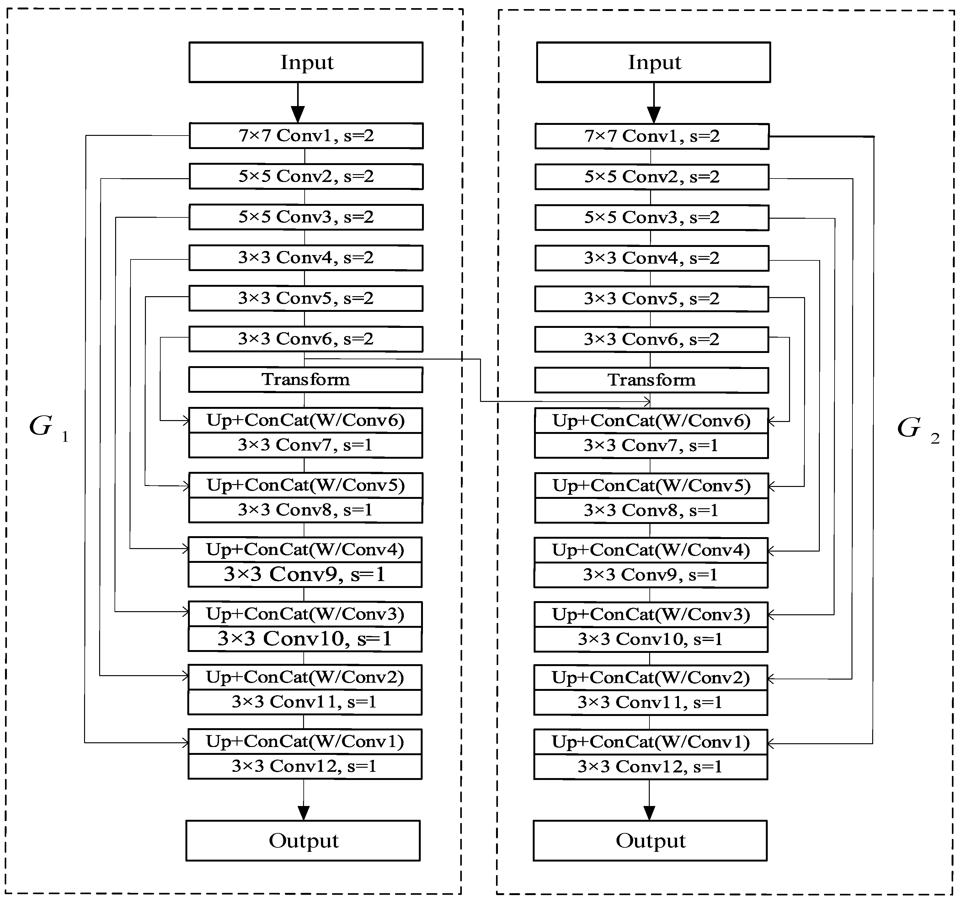
The image inpainting network is implemented as a Generative Adversarial Network, where two generators generate texture and structure information, respectively, modeled by a U-Net variant. As shown in Figure 1, both texture and structure generators are encoded–decoded structures, and a structure discriminator and texture discriminator are designed to distinguish the real image from the generated image by estimating the texture and structure features, respectively. The image generated by the generator is sent to the discriminator, together with the real image. The discriminator outputs “True” if the image is real and “False” if the image is generated, prompting the generator to generate images that are similar to the real ones. The structure of the two-stage inpainting network is shown in Figure 1.
A transform module based on cross-aggregation of windows is embedded to improve the information aggregation between the windows, without increasing the computational complexity. This improves the aggregation of information between the windows, allowing the effective acquisition of distant image dependencies. This solves the problem that the convolution operation is limited by local feature extraction. The two parallel coupled streams are modeled separately and combined to complement each other, further improving the structural and textural integrity of the generated images.
The two-stage network is described in detail below:

3.1.1. Generator Network

The two-stage image inpainting network uses dual generators, which are a structure generator and a texture generator. In this paper, the inpainting algorithm has different tasks depending on the mask area. In general, it can be seen to complement high-frequency information (structure) and low-frequency information (texture) modeled by a U-Net variant with an encoded–decoded form. This paper uses a dilated convolutional kernel instead of a partially normal convolutional kernel, with the kernel proposed in [34]. This choice simultaneously alleviates the problems of gradient dispersion and gradient explosion, while generating more complex predictions by combining low-level and high-level features at multiple scales through jump connections. The details of the generator structure are shown in Figure 2.

3.1.2. Dual Discriminators

Both the structure discriminator D 1 and the texture discriminator D 2 are selected as spectrally normalized Markov discriminators. The structural parameters are shown in Table 1.
However, the structure discriminator and the texture discriminator also differ significantly. The former takes into account the enhancement of its own adversarial loss, which is achieved by inputting pairs of data. In terms of the input data, there are two main points: firstly, the edge map of the fused image derived using the edge detection algorithm, and secondly, the grayed-out image. After the above optimization steps, the structure discriminator is able to steadily improve the similarity between the restored image and the original image, and at the same time, it is able to discriminate whether the structured texture of the restored image is real or not.
The image inpainting algorithm of the two-stage network is divided into three steps to complete the inpainting:
(1) Pre-processing (edge detection). The edge information of the broken image is the prerequisite for the inpainting algorithm. The discovered excellent edge detection algorithm [35] is fused into our proposed two-stage image inpainting algorithm to make it perform the high-precision edge detection of the input broken image before inpainting.
(2) Structure and texture repair. The detected broken edge image, grayscale image, and mask are inputted into the structure encoding generator together to generate a preliminary complete structure image. The complete edge image is inputted into the texture repair generator network together with the broken image to generate a preliminary complete texture image.
(3) The initial structural and textural image information are fused to obtain the complete image, which is then discriminated by the structural discriminator D 1 and textural discriminator D 2 . If the generated image is determined as being false, the information is fed back to the generator, and the generator is prompted to adjust the network parameters to generate an image that is more similar to the real image. This iterative process ends when both D 1 and D 2 are unable to distinguish between true and false images.

3.1.3. Aggregation Transform

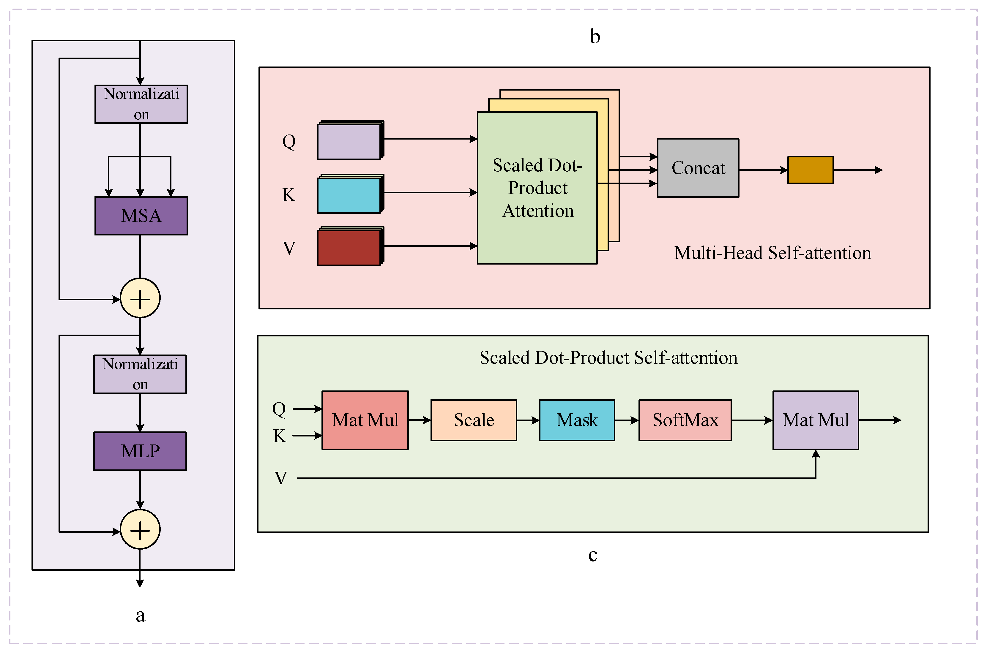
The transformer [36] omits recursion and convolution and follows an encoder–decoder structure, where the encoder consists of six identical layers, the structure of which is shown in Figure 3, with two sub-layers each. The first layer is a multi-headed self-attentive mechanism, and the second layer is a simple multilayer perceptron. Residual connectivity [37] was used around each of the two sub-layers, followed by layer normalization [38]. The decoder is similar in structure to the encoder in that it also contains six identical layers, with each decoder layer having three sub-layers. The difference is that the attention mechanism layer is embedded in the decoder, ensuring that the prediction of position i depends only on the known output with positions less than i.
The structure of the multi-head self-attentive mechanism and the self-attentive mechanism are shown in Figure 3b,c. For the self-attentive mechanism, the three matrices Q (Queries), K (Keys) and V (Values) all come from the same input, and the calculation formula is shown in (1).
Attention ( Q , K , V ) = SoftMax ( Q K T d k ) V
where Q K T d k counts the raw score of attention (which is actually the similarity score derived from the dot product of Q and K ). d k is a scaling factor that keeps the result from being too large or too small and avoids it being either 0 or 1 after softmax.
In the transformer, the self-attentive layer is further refined by adding a multi-headed attention mechanism by first mapping the Queries, Keys, and Values by h different linear transformations. Then, the different attentions are stitched together. Finally, a linear transformation is performed. Each set of attention is used to map the input them into a different sub-representation space, which allows the network model to jointly pay attention to the subspace feature information under different representatives of Queries, Keys, and Values at the same location, while acquiring more detailed features; the computational process can be expressed as:
MultiHead ( Q , K , V ) = Concat ( h e a d 1 , , h e a d i ) W o
h e a d n = Attention ( Q W n Q , K W n K , V W n V )
where W n Q R d mod e l × d q , W n K R d mod e l × d K , and W n V R d mod e l × d V are the Queries, Keys, and Values of the projection matrix with head number k . All the heads h e a d 1 , , h e a d i are connected for linear projection to obtain the final result.

3.1.4. The Joint Loss Function

The two-stage inpainting network employs semantic-based joint loss training, including feature content loss, reconstruction loss, perceptual loss, style loss, and adversarial loss. By combining the above various loss functions, a complementary effect is achieved, which ultimately enables the restored images generated by the inpainting network to meet not only the visual match with the original image, but also the high accuracy requirements when the hard evaluation of metrics is performed.
(1)
Feature content loss
The feature content loss L f stabilizes the training process by comparing the activation mappings in the middle layer of the discriminator D to constrain the generator G to produce results that are more similar to the true structure map.
L f = E i = 1 n 1 N i D i ( E i n ) D i ( E o u t ) 1
where n denotes the total number of convolutional layers of discriminator D , N i is the number of elements of the i-th layer, and D i denotes the activation function output of the i-th layer of discriminator D .
(2)
Reconstruction loss
The normalized L 1 distance is generally used as the reconstruction loss; however, in this paper, we use the distance L 1 between I o u t and I g t as the reconstruction loss, with the following equation:
L r e c = I o u t I g t 1
(3)
Perceptual loss [39]
In order to preserve the structural information of the global image and ensure the similarity of the high-level structure, image restoration requires a feature representation similar to that of the real image, rather than just pixel matching between images. The perceptual loss is calculated using a VGG-16 feature extractor [40] pre-trained on the ImageNet dataset [41] to extract the feature maps of the generated and real images separately and based on the L 1 distance between them; it is defined as follows:
L p e r c = E i ϕ i ( I o u t ) ϕ i ( I g t ) 1
where ϕ i ( · ) denotes the activation mapping obtained for a given input image I * through the i-th pooling layer of VGG-16.
(4)
Style loss
The perceptual loss helps to obtain a higher-level structure and avoid the generated image from deviating from the real image. In order to maintain the style consistency, this paper adds style loss to the joint loss function. The style loss calculates the L 1 distance of the Gram matrix of the feature map generated by the image after VGG-16. The perceptual loss defined as follows:
L s t y l e = E i G r a m φ i ( I o u t ) G r a m φ i ( I g t ) 1
where G r a m denotes the Clem matrix, G r a m φ i ( · ) = ϕ i ( · ) T ϕ i ( · ) .
(5)
Adversarial loss [42]
Adversarial loss is used to enhance the gaming process of the generative and discriminative networks, aiming to make the data distribution of the generated image more similar to the real image, making the result more realistic. The objective function of the discriminative network is used here, which is defined in Equation (8) is shown as follows:
L a d v = min G   max D   E I g t , E g t log D ( I g t , E g t ) + E I o u t , E o u t log 1 G ( I o u t , E o u t )
In summary, the joint loss function is as follows:
L j o i n t = λ 1 L f + λ 2 L r e c + λ 3 L p e r c + λ 4 L s t y l e + λ 5 L a d v
where λ 1 = 10 , λ 2 = 10 , λ 3 = 0.1 , λ 4 = 250 , λ 5 = 0.1 .

3.2. Training of the Model

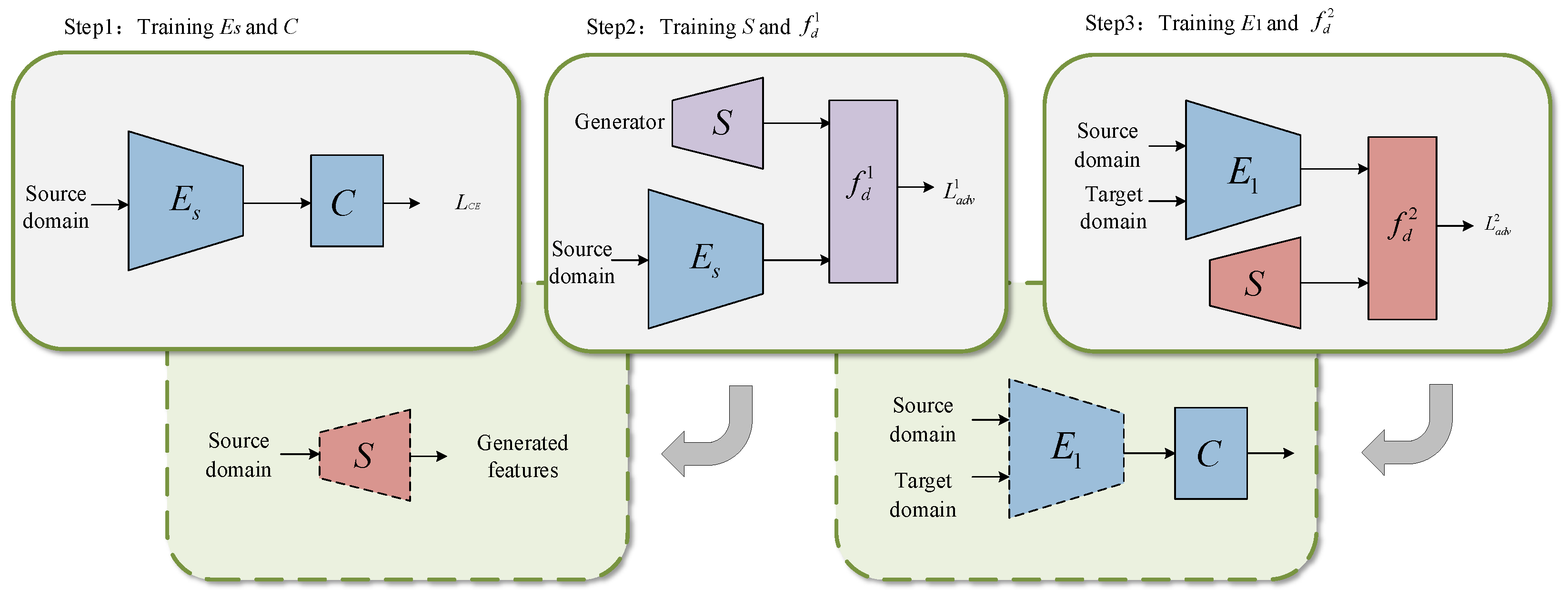
A large public dataset is used as the source domain, and the old photo dataset is used as the target domain, and the training process is made smoother by adding data to the source domain. The goal of this transfer learning is to train a domain-invariant feature extractor, and the training is divided into three main steps, as shown in Figure 4. The solid line indicates that the modules are being trained, and the dashed line indicates the trained models.
In the first step, this model is decoupled into a feature extractor E and a classifier C , which are an encoder and a decoder, respectively. During training E S , one performs feature extraction on the source domain samples, and C denotes the fully connected Softmax layer. Minimized cross-entropy loss is used.
L C E = min θ E s , θ C E ( x i ) ~ ( X s ) H ( C E s ( x i ) )
where θ E s and θ C denote the parameters of E S and C, respectively, X s denotes the distribution of samples in the source domain, and H denotes the softmax cross-entropy function.
In the second step, the model S is trained to generate feature generators similar to the source domain features, and then training is performed using adversarial loss, as exemplified by the structural generation:
L a d v 1 = min θ S   max θ f d 1   E ( z , e i ) ~ ( p z ( z ) , E i ) f d 1 ( S ( z e i ) e i ) 1 2 + E ( e i , x i ) ~ ( E i , X i ) f d 1 ( E s ( x i ) e i ) 2
where θ S and θ f d denote the parameters of S and f d , respectively, p z ( z ) is the sample distribution extracted from e , and e is the edge feature vector. In order to generate an arbitrary number of new feature samples, it is only necessary for S to take a cascade of noise vectors and an edge feature as an input and to output the desired generated feature vector:
F ( z | e ) = S ( z e )
where z ~ p z ( z ) and F are feature vectors belonging to e.
In the third step, after initialization using the weights optimized in step one, the following maximum minimum training domain-invariant encoder E 1 is obtained to achieve optimal convergence.
L a d v 2 = min θ E 1   max θ f d 2   E x i ~ X s X t f d 2 ( E 1 ( x i ) ) 1 2 + E ( z , e i ) ~ ( p z ( z ) , E i ) f d 2 ( S ( z e i ) ) 2
where θ E 1 and θ f d 2 denote the parameters of E 1 and f d 2 , respectively. Since the model E 1 is trained using source and target domains, the results of the feature extractor are domain-invariant. It maps source and target samples in a common feature space, where features are indistinguishable from those generated using S. Since the latter is trained to produce features indistinguishable from the source samples, the feature extractor can be combined with the encoder of step one for image structure feature generation, and the texture generator is consistent with the above steps.

4. Experimental Analysis

4.1. Analysis of Experimental Results of Inpainting Model

We used the CelebA and Places datasets, which are widely used in the literature, to evaluate the proposed approach. We selected 10 categories from Places, each with 5000 training images, 900 test images, and 100 validation images. We used 30,000 images for training and 10,000 images for testing. The mask datasets for the experiments all used irregular masks obtained from [43], classified according to their hole size relative to the whole image in 10% increments; all images and corresponding masks were adjusted to 256 × 256 pixels, the batch size processed was 16 sheets, and 300,000, training iterations were used, optimized using the Adam optimizer [44] with the parameters set to β 1 = 0.001 and β 2 = 0.9 . The model was first initially trained using a learning rate of 2 × 10⁻⁴, and then fine-tuned with a learning rate of 5 × 10⁻⁵, and the BN layer of the generator was frozen, and the discriminator was trained with a learning rate of 1/10 of the generator. The deep learning framework used for the experiments was Pytorch, the computer operating system was Windows 10, and the graphics card model was NVIDIA TITAN XP with 12G of video memory.

4.1.1. Qualitative Analysis

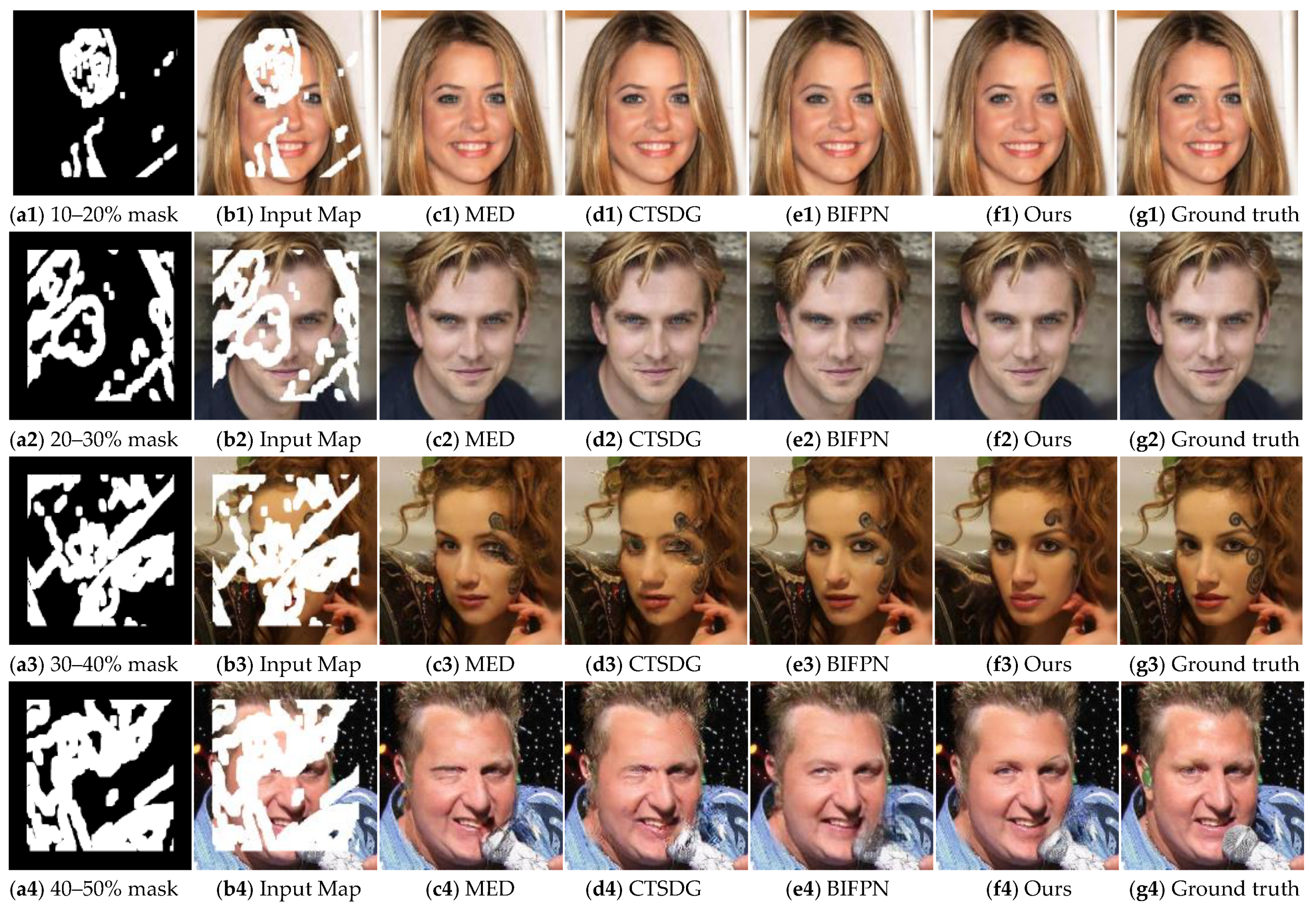
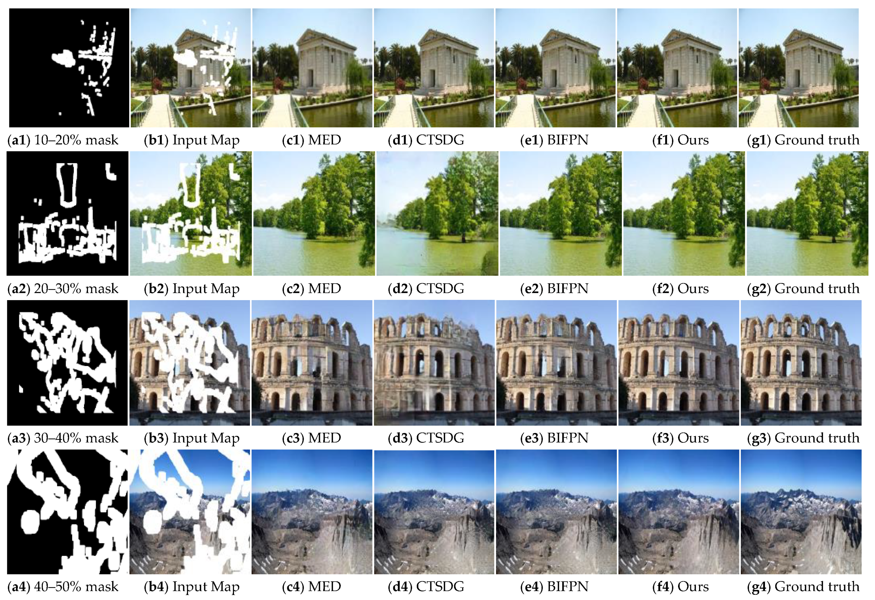
To verify the effectiveness of the two-stage image inpainting network proposed in this paper, test sets of the CelebA dataset and the Places dataset were used to compare the subjective as well as numerical results of this paper’s method with the MED [21], CTSDG, and BIFPN algorithms. Figure 5 shows the inpainting results of the method in this paper on the CelebA datasets.
Figure 5 shows the inpainting results of MED, CTSDG, BIFPN, and the methods proposed in this paper for different mask rates on the CelebA dataset. It can be observed that all the inpainting methods show a good performance when the mask area is small, specifically when the mask area is 10–20% of the original size, with only minor differences between the original and inpainted result maps. The MED and CTSDG methods (subfigure c2 and subfigure d2, respectively) exhibit varying degrees of blurring at 20–30% of the masked area, whereas the proposed methods maintain good inpainting, with sharper textural and structural properties. At a mask area of 30–40%, the MED, CTSDG, and BIFPN methods (subfigure c3, subfigure d3, and subfigure e3, respectively) all exhibit artifacts and even facial distortions, with some facial features being lost. Although the proposed algorithm also exhibits blurring and distortion, it still yields better inpainting results compared with those of the other three methods. At 40–50% of the masked area, it becomes clear that the restored image from the inpainting other algorithms is significantly distorted and no longer conveys the texture information that the original image should. In contrast, the proposed algorithm maintains a large amount of texture detail, with only a few differences with the ground truth.
Figure 6 shows the inpainting results of MED, CTSDG, BIFPN, and the proposed methods for different mask rates on the Places dataset. It can be observed that most of the inpainting methods show a good performance when the mask area is between 10–20% of the original size, with only MED exhibiting significant distortion. At a mask area of 20–30%, the image itself shows good inpainting due to its characteristics (e.g., the structure information is not obvious), but a detailed comparison reveals that the proposed method yields a clearer texture and structure inpainting performance. At a mask area of 30–40%, the MED, CTSDG, and BIFPN methods (subfigure c3, subfigure d3, and subfigure e3, respectively) exhibit artifacts and even facial distortions, with some image features being lost. At a mask area of 40–50%, it is evident that the remaining three algorithms have lost too many landscape details, with a significant portion of the area lacking texture details, which is significantly different from the results obtained by the proposed algorithm.

4.1.2. Quantitative Analysis

We refer to all the current studies in the field related to image inpainting and decide to adopt the three types of metrics, PSNR, SSIM, and FID, which were all used in quantitative evaluation to evaluate our restored images. At the same time, we designed the comparison experiments with other algorithms, and all algorithms used mask rates in inpainting based on 10–20% with 10% increments. Ultimately, the comparison of the quantitative analysis results clearly shows that the inpainting performance of our proposed algorithm model is much better than that of the other algorithms. The quantitative results of the three metrics for each specific algorithm are shown in Table 2 and Table 3.
From Table 2, it can be seen that the MED algorithm is clearly at a disadvantage when it needs to deal with the task of CelebA image inpainting at different mask rates. While our proposed algorithm model has its own advantages over the remaining two algorithms when facing different mask rates, it can be found that the model in this paper still significantly outperforms the rest of the algorithms, and this phenomenon can be clearly seen when targeting the image inpainting task of CelebA with high mask rates.
As for the Places dataset in natural scenes, Table 3 shows that the SSIM metrics of our proposed image inpainting model are slightly lower than those of the BIFPN model only at the mask rate interval of 10–20%. When restoration is performed at the rest of the mask rates, the restoration performance of our proposed inpainting model outperforms the rest of the algorithms, and the effect is especially prominent at high mask rates.
In summary, our algorithm outperforms current state-of-the-art image inpainting models.

4.2. Analysis of Old Photo Inpainting Results with Transfer Learning

In this paper, a modified two-stage image inpainting network is used as the base network by employing a model initialized using pre-trained source domain data in the initialization phase of the model. The pre-trained source domain model is trained on the CelebA dataset to obtain the weights. For training, the learning rate of all the fine-tuning layer parameters was 0.1 times the learning rate of the training layer parameters, using an Adam optimizer with momentum set to 0.95. The domain discriminators all use three fully connected layers and the ReLU activation layer. L2 regularization was also used for all the parameters with a factor of 0.1. In order to obtain a more stable representation of the data distribution, the data batch size is set to six for each iteration, and the number of model training iterations is based on the number of traversals of the small dataset, with the maximum number of traversals being 100. The mask dataset used in transfer learning training adopts the irregular mask obtained from [43]. In order to restore the old photo image more realistically, the mask used in the test experiment is extracted from the damaged old photo.

4.2.1. Experimental Content

In order to verify the practicality of the feasibility and effectiveness of transfer learning on old photo image inpainting tasks, we have prepared corresponding comparative experiments. Both sets of experiments used a two-stage inpainting network as the base network, and both sets of experiments were as follows:
Group 1 (without transfer learning): The hybrid dataset was used as the training data for the model, and the model was trained directly without transfer learning, when all the parameters in the model were initialized. (The hybrid dataset is the sum of the CelebA training set and the old photo training set).
Group 2 (using transfer learning): This group was training using transfer learning, and the steps are shown in Figure 4.

4.2.2. Dataset Acquisition and Pre-Processing

In the experiments and results analysis in this paper, it can be concluded that our proposed image inpainting model can obtain a good image inpainting performance; however, when the trained model is applied to the old photo inpainting task, it was found that the model does not restore the old photos well. After analysis, the main reason for the poor robustness of the model is that the open-source dataset is not exactly in the same style as the old photo dataset. Old photographs are subject to fading and blurring due to the limitations of past filming equipment and preservation conditions, and there are significant differences between them and the images obtained from the open-source dataset.
Due to the sparse sample of old photo image dataset, a transfer learning approach is used to implement the task of inpainting of old photos. A total of 316 images of complete old photo faces were collected from the internet, and 91 images of broken or blurred old photos were obtained after screening. The complete old photo images were divided into a training set, a validation set, and a test set in a ratio of approximately 8:1:1, and the results are shown in Table 4:
We use the random mask in this paper for training, and in order to make the broken old photos more realistic, the test mask for old photo inpainting uses the broken mask detected from the real broken old photo images as the test mask.

4.2.3. Analysis of Experimental Results

As the core work in this subsection is the task of old photo images inpainting, a subjective comparison was carried out with a focus on the overall inpainting of old photos.
  • Subjective evaluation
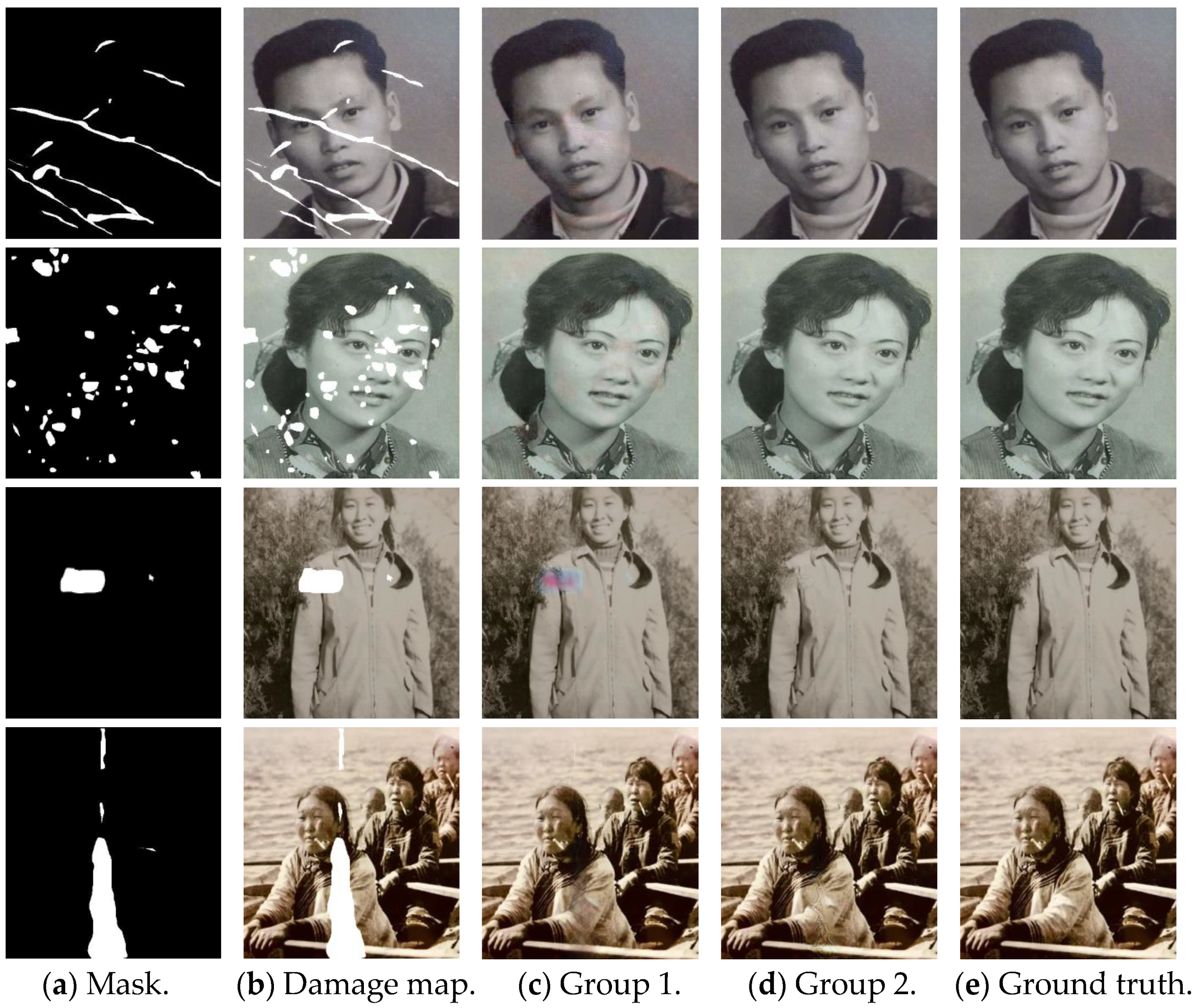
An example plot of the comparison results for the first and second groups, respectively, on the old photo dataset is shown below, as shown in Figure 7.
As can be seen in Figure 7, the inpainting results for the first group have significant pixel inconsistencies, as seen in the third row where the shoulders appear to be colored, and in the second row where inconsistent facial colors are observed for the faces. On the other hand, the second group of inpainting results have better consistency, and it can be seen that the inpainted images are largely visually unobstructed.
In summary, the use of transfer learning methods in old photo image inpainting tasks gives more stability and accuracy in the results in terms of structural and texture features. It can produce more realistic results with more natural facial features for face images.
2.
Objective evaluation
In order to more objectively evaluate the strengths and weaknesses of the algorithms used in this paper, quantitative analysis experiments were set up. The inpainting results of the two groups of methods were quantitatively analyzed, and the experimental mask used the broken mask detected from the real broken old photo images as the test mask, and the test masks were consistent in both groups, and the quantitative results are shown in Table 5.
From Table 5, it can be concluded that the use of transfer learning can make the inpainting of old photos more natural, and both PSNR and SSIM are far better than those without the use of transfer learning, which is basically consistent with the results of the qualitative analysis, thus proving the effectiveness of using the method of transfer learning in the inpainting of old photos images.

5. Discussion

At the early stage of the COVID-19 outbreak, it was not possible to conduct relevant research using neural networks because of the sparse dataset samples and the need for neural networks to rely on a large number of datasets for training. Due to this, in this paper, the authors applied transfer learning to the field of image inpainting for the first time. Specifically, the authors took the inpainting of old photo images as the research object, constructed a two-stage image inpainting model, and embedding Transform into the generator in the form of residual blocks, which solves the problem of long-distance feature acquisition that cannot be achieved by convolution. The generator was decoupled into a feature extractor and a classifier, and a domain-invariant feature extractor was trained with a large public dataset as the source domain and an old photo image as the target domain. Experimentally, the application of transfer learning to image inpainting in this paper has achieved initial success and proved the effectiveness of the method. And this work in this paper also provides new ideas for the subsequent research of image inpainting techniques for small sample datasets, so that it can be satisfied with more application scenarios.

6. Conclusions

In this paper, we introduce transfer learning techniques to address the problem of sparse samples of old photo datasets. In order to build an inpainting network more suitable for transfer learning, a two-stream network is decoupled into two parallel streams to form a two-stage network based on the original two-stream structure of the image inpainting model. A dual discriminator is designed to give the model a better inpainting performance by estimating texture and structure separately. Secondly, using a two-stage image inpainting network as the base model, the generator is decoupled into a feature extractor and a classifier, which are an encoder and a decoder, respectively, and a domain-invariant feature extractor is obtained by training the source and target domain data, which can be combined with the original encoder for the inpainting task of old photo images. The experiments show that the inpainting of old photos using transfer learning is better than that without transfer learning, maintaining pixel consistency and reasonableness. In the qualitative experimental analysis, the PSNR, SSIM, and FID indexes of the model using transfer learning are 11.8%, 2.96%, and 44.4% higher than those without transfer learning, respectively.

Author Contributions

M.C. designed the two-stage inpainting network and verified the feasibility of the model by verification; Z.D. proposed the idea of transfer learning inpainting of old photos and conducted transfer learning experiments using the model; S.Y. derived the results of the comparison algorithms and compared them with the method in this paper; A.C. wrote the overall article; L.L. translated and checked the full article and provided the server required for the experiments, etc. All authors have read and agreed to the published version of the manuscript.

Funding

This research was funded by Natural Science Foundation of Sichuan, China (2023NSFSC1987, 2022ZHCG0035); The Opening Fund of Artificial Intelligence Key Laboratory of Sichuan Province (2020RZY03); The Key Laboratory of Internet Information Retrieval of Hainan Province Research Found (2022KY03); The Opening Project of International Joint Research Center for Robotics and Intelligence System of Sichuan Province (JQZN2022-005); Sichuan University of Science & Engineering Postgraduate Innovation Fund Project (Y2022132).

Institutional Review Board Statement

Not applicable.

Informed Consent Statement

Not applicable.

Data Availability Statement

Data are contained within the article.

Conflicts of Interest

The authors declare no conflict of interest.

Abbreviations

GAN (Generative Adversarial Network); EC (EdgeConnect); MED (Mutual Encoder-Decoder); CTSDG (Conditional Texture and Structure Dual Generation); BIFPN (Bi-directional Feature Pyramid Network); PSNR (Peak Signal-to-Noise Ratio); SSIM (Structural Similarity Index Measure); FID (Frechet Inception Distance score).

References

  1. Criminisi, A.B.; Perez, P.; Toyama, K. Region Filling and Object Removal by Exemplar-Based Image Inpainting. IEEE Trans. Image Process. 2004, 13, 200–1212. [Google Scholar] [CrossRef]
  2. Li, L.; Chen, M.J.; Shi, H.D.; Duan, Z.X.; Xiong, X.Z. Multiscale Structure and Texture Feature Fusion for Image Inpainting. IEEE Access 2022, 10, 82668–82679. [Google Scholar] [CrossRef]
  3. Bertalmio, M.; Sapiro, G.; Caselles, V.; Ballester, C. Image Inpainting. In Proceedings of the 27th Annual Conference on Computer Graphics and Interactive Techniques, New Orleans, LA, USA, 23–28 July 2000; pp. 417–424. [Google Scholar]
  4. Levin, A.; Zomet, A.; Weiss, Y. Learning how to inpaint from global image statistics. In Proceedings of the ICCV, Nice, France, 13–16 October 2003; pp. 305–312. [Google Scholar]
  5. Li, L.; Chen, M.J.; Xiong, X.Z.; Yang, Z.W.; Zhang, J.S. A Continuous Nonlocal Total Variation Image Restoration Model. Radio Eng. 2021, 51, 864–869. [Google Scholar]
  6. Darabis, S.; Shechtman, E.; Barnes, C.; Goldman, D.B.; Sen, P. Image melding: Combining inconsistent images using patch-based synthesis. ACM Trans. Graph. 2021, 31, 4. [Google Scholar] [CrossRef]
  7. Efrosa, A.; Freemanw, T. Image quilting for texture synthesis and transfer. In Proceedings of the 28th Annual Conference on Computer Graphics and Interactive Techniques, New York, NY, USA, 12–17 August 2001; pp. 341–346. [Google Scholar]
  8. Yeh, R.A.; Chen, C.; Lim, T.Y.; Schwing, A.G.; Hasegawa-Johnson, M.; Do, M.N. Semantic image inpainting with deep generative models. In Proceedings of the ICCV, Venice, Italy, 22–29 October 2017; pp. 6882–6890. [Google Scholar]
  9. Goodfellow, I.J.; Pouget-Abadie, J.; Mirza, M.; Xu, B.; Warde-Farley, D.; Ozair, S.; Courville, A.; Bengio, Y. Generative adversarial nets. In Proceedings of the NIPS, Montreal, BC, Canada, 8–13 December 2014; pp. 2672–2680. [Google Scholar]
  10. Yu, X. Research on Face Image Inpainting Method Based on Generative Adversarial Network. Master’s Thesis, Southwest University of Science and Technology, Mianyang, China, 2022. [Google Scholar] [CrossRef]
  11. Deepak, P.; Philipp, K.; Jeff, D.; Darrell, T.; Efros, A.A. Context encoder: Feature Learning by Inpainting. In Proceedings of the CVPR, Las Vegas, NV, USA, 26 June–1 July 2016. [Google Scholar] [CrossRef] [Green Version]
  12. Jason, Y.; Jeff, C.; Yoshua, B.; Lipson, H. How transferable are features in deep neural networks? In Proceedings of the NIPS, Montreal, BC, Canada, 8–13 December 2014. [Google Scholar] [CrossRef]
  13. Zeiler, M.D.; Rob, F. Visualizing and under-standing convolutional networks. In Proceedings of the ECCV, Zurich, Switzerland, 6–12 September 2014. [Google Scholar]
  14. Azizpour, H.; Razavian, A.S.; Sullivan, J.; Maki, A.; Carlsson, S. Factors of transferability for a generic convnet representation. IEEE Trans. Pattern Anal. Mach. Intell. 2016, 38, 1790–1802. [Google Scholar] [CrossRef] [PubMed] [Green Version]
  15. Zhao, M.; Kang, M.; Tang, B.; Pecht, M. Deep residual networks with dynamically weighted wavelet coefficients for fault diagnosis of planetary gearboxes. IEEE Trans. Ind. Electron. 2017, 65, 4290–4300. [Google Scholar] [CrossRef]
  16. Nazeri, K.; Ng, E.; Joseph, T.; Qureshi, F.; Ebrahimi, M. Edgeconnect: Structure guided image inpainting using edge prediction. In Proceedings of the 2019 IEEE/CVF International Conference on Computer Vision Workshop (ICCVW), Seoul, Republic of Korea, 27–28 October 2019. [Google Scholar]
  17. Xiong, W.; Yu, J.; Lin, Z.; Yang, J.; Lu, X.; Barnes, C.; Luo, J. Foreground-aware image inpainting. In Proceedings of the 2019 IEEE Conference on Computer Vision and Pattern Recognition (CVPR), Long Beach, CA, USA, 15–20 June 2019. [Google Scholar]
  18. Ren, Y.; Yu, X.; Zhang, R.; Li, T.H.; Liu, S.; Li, G. Structureflow: Image inpainting via structure-aware appearance flow. In Proceedings of the 2019 IEEE/CVF International Conference on Computer Vision (ICCV), Seoul, Republic of Korea, 27 October–2 November 2019. [Google Scholar]
  19. Li, J.; He, F.; Zhang, L.; Du, B.; Tao, D. Progressive reconstruction of visual structure for image inpainting. In Proceedings of the 2019 IEEE/CVF International Conference on Computer Vision (ICCV), Seoul, Republic of Korea, 27 October–2 November 2019. [Google Scholar]
  20. Yang, J.; Qi, Z.Q.; Shi, Y. Learning to incorporate structure knowledge for image inpainting. In Proceedings of the AAAI Conference on Artificial Intelligence, New York, NY, USA, 7–12 February 2020. [Google Scholar]
  21. Liu, H.; Jiang, B.; Song, Y.; Huang, W.; Yang, C. Rethinking image inpainting via a mutual encoder-decoder with feature equalizations. In Proceedings of the 16th European Conference on Computer Vision (ECCV), Glasgow, UK, 23–28 August 2020. [Google Scholar]
  22. Guo, X.; Yang, H.; Huang, D. Image Inpainting via Conditional Texture and Structure Dual Generation. In Proceedings of the 2021 IEEE/CVF International Conference on Computer Vision (ICCV), Montreal, BC, Canada, 11–17 October 2021; pp. 14114–14123. [Google Scholar]
  23. Liu, H.; Wan, Z.; Huang, W.; Song, Y.; Han, X.; Liao, J. PD-GAN: Probabilistic diverse GAN for image inpainting. In Proceedings of the 2021 IEEE/CVF Conference on Computer Vision and Pattern Recognition (CVPR), Nashville, TN, USA, 20–25 June 2021; pp. 9367–9376. [Google Scholar]
  24. Tan, C.; Sun, F.; Kong, T.; Zhang, W.; Yang, C.; Liu, C. A survey on deep transfer learning. In Proceedings of the International Conference on Artificial Neural Networks, Barcelona, Spain, 5–7 October 2018; pp. 270–279. [Google Scholar]
  25. Ge, W.F.; Yu, Y.Z. Borrowing treasures from the wealthy: Deep transfer learning through selective joint fine-tuning. In Proceedings of the ICCV, Venice, Italy, 22–29 October 2017; pp. 1086–1095. [Google Scholar]
  26. Cui, Y.; Song, Y.; Sun, C.; Howard, A.; Belongie, S. Large scale fine-grained categorization and domain-specific transfer learning. In Proceedings of the CVPR, Salt Lake City, UT, USA, 18–23 June 2018; pp. 4109–4118. [Google Scholar]
  27. Long, M.; Cao, Y.; Wang, J.; Jordan, M. Learning transferable features with deep adaptation networks. In Proceedings of the International Conference on Machine Learning, Lille, France, 7–9 July 2015; pp. 97–105. [Google Scholar]
  28. Tzeng, E.; Hoffman, J.; Zhang, N.; Saenko, K.; Darrell, T. Deep domain confusion: Maximizing for domain invariance. arXiv 2014, arXiv:1412.3474. [Google Scholar] [CrossRef]
  29. Gretton, A.; Borgwardt, K.M.; Rasch, M.J.; Schölkopf, B.; Smola, A. A kernel two-sample test. J. Mach. Learn. Res. 2012, 13, 723–773. [Google Scholar]
  30. Haeusser, P.; Frerix, T.; Mordvintsev, A.; Cremers, D. Associative domain adaptation. In Proceedings of the ICCV, Venice, Italy, 22–29 October 2017. [Google Scholar]
  31. Chen, H.; Zhang, Z.; Deng, J.; Yin, X. A Novel Transfer-Learning Network for Image Inpainting. In Proceedings of the ICONIP, Sanur, Bali, Indonesia, 8–12 December 2021; pp. 20–27. [Google Scholar]
  32. Zhao, Y.M.; Zhang, Y.X.; Sun, Z.S. Unsupervised Transfer Learning for Generative Image Inpainting with Adversarial Edge Learning. In Proceedings of the 2022 5th International Conference on Sensors, Signal and Image Processing, Birmingham, UK, 28–30 October 2022; pp. 17–22. [Google Scholar]
  33. Li, L.; Chen, M.J.; Shi, H.D.; Liu, T.T.; Deng, Y.S. Research on Image Inpainting Algorithm Based on BIFPN-GAN Feature Fusion. Radio Eng. 2022, 52, 2141–2148. [Google Scholar]
  34. Yu, F.; Koltun, V. Multi-scale Context Aggregation by Dilated Convolutions. arXiv 2015, arXiv:1511.07122. [Google Scholar]
  35. Lou, L.; Zang, S. Research on Edge Detection Method Based on Improved HED Network. J. Phys. Conf. Ser. 2020, 1607, 012068. [Google Scholar] [CrossRef]
  36. Vaswani, A.; Shazeer, N.; Parmar, N.; Uszkoreit, J.; Jones, L.; Gomez, A.N.; Kaiser, Ł.; Polosukhin, I. Attention is all you need. In Proceedings of the NIPS, Long Beach, CA, USA, 4–9 December 2017; pp. 5998–6008. [Google Scholar]
  37. He, K.; Zhang, X.; Ren, S.; Sun, J. Deep residual learning for image recognition. In Proceedings of the CVPR, Las Vegas, NV, USA, 27–30 July 2016; pp. 770–778. [Google Scholar]
  38. Jimmy, L.B.; Jamie, R.K.; Geoffrey, E.H. Layer normalization. arXiv 2016, arXiv:1607.06450. [Google Scholar] [CrossRef]
  39. Johnson, J.; Alahi, A.; Fei-Fei, L. Perceptual losses for real-time style transfer and super-resolution. In Proceedings of the ECCV, Amsterdam, The Netherlands, 11–14 October 2016. [Google Scholar]
  40. Jia, D.; Wei, D.; Socher, R.; Li, L.J.; Li, K.; Fei-Fei, L. ImageNet: A large-scale hierar-chical image database. In Proceedings of the CVPR, Miami, FL, USA, 20–25 June 2009; pp. 248–255. [Google Scholar]
  41. Simonyan, K.; Zisserman, A. Very deep convolutional net-works for large-scale image recognition. arXiv 2014, arXiv:1409.1556. [Google Scholar] [CrossRef]
  42. Jolicoeur-Martineau, A. The relativistic discriminator: A key element missing from standard GAN. In Proceedings of the ICLR, Vancouver, BC, Canada, 30 April–3 May 2018. [Google Scholar]
  43. Liu, G.; Reda, F.A.; Shih, K.J.; Wang, T.C.; Tao, A.; Catanzaro, B. Image Inpainting for Irregular Holes Using Partial Convolutions. In Proceedings of the ECCV, Munich, Germany, 8–14 September 2018; pp. 85–100. [Google Scholar]
  44. Kingma, D.; Ba, J. Adam: A Method for Stochastic Optimization. arXiv 2014, arXiv:1412.6980. [Google Scholar] [CrossRef]
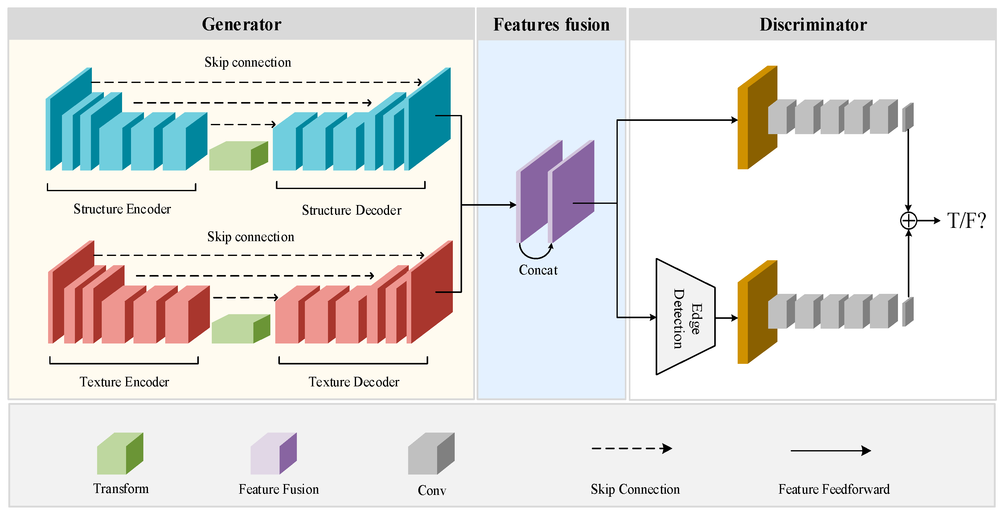
Figure 1. Structure of two-stage image inpainting network.
Electronics 12 03221 g001
Figure 2. Generator structure detail diagram.
Electronics 12 03221 g002
Figure 3. The framework structure of transformer. (a) Aggregation Transformer; (b) Multi-Head Self-attention; (c) Scaled Dot-Product Self-attention.
Electronics 12 03221 g003
Figure 4. Training procedure.
Electronics 12 03221 g004
Figure 5. Comparison of qualitative analysis results on CelebA.
Electronics 12 03221 g005
Figure 6. Comparison of qualitative analysis results on Places.
Electronics 12 03221 g006
Figure 7. Comparison of qualitative analysis results on old photo datasets.
Electronics 12 03221 g007
Table 1. Details of the structure of the discriminator network.
Layers NamesConvolution Kernel SizeStep SizeActivation FunctionOutput Feature Maps
Convolutional layer 14 × 42LeakyReLU64 × 128 × 128
Convolutional layer 24 × 42LeakyReLU128 × 64 × 64
Convolutional layer 34 × 42LeakyReLU256 × 32 × 32
Convolutional layer 44 × 41LeakyReLU512 × 16 × 16
Convolutional layer 54 × 41LeakyReLU512 × 4 × 4
Fully connected layer--Sigmoid512 × 1 × 1
Table 2. Comparison of quantitative analysis results on CelebA.
Mask RateMEDCTSDGBIFPNOurs
PSNR↑10–20%28.7532.6732.1132.03
20–30%26.9728.1328.6728.44
30–40%23.6725.3225.8126.43
40–50%22.0723.4623.5624.79
SSIM↑10–20%0.9220.9580.9600.953
20–30%0.9040.9170.9240.931
30–40%0.8370.8520.8630.882
40–50%0.8110.8260.8330.841
FID↓10–20%5.632.612.672.95
20–30%6.793.743.243.11
30–40%8.645.355.024.78
40–50%9.117.697.637.11
Table 3. Comparison of quantitative analysis results on Places.
Mask RateMEDCTSDGBIFPNOurs
PSNR ↑10–20%28.0530.5431.0931.86
20–30%25.4426.5526.6127.14
30–40%22.8923.7324.1725.71
40–50%21.7622.5422.7823.64
SSIM ↑10–20%0.9240.9290.9340.926
20–30%0.8740.8970.9060.907
30–40%0.8460.8560.8620.873
40–50%0.8110.8260.8340.842
FID ↓10–20%5.714.113.883.16
20–30%6.595.214.164.07
30–40%9.147.687.116.89
40–50%11.549.138.758.18
Table 4. Old photo images segmentation dataset.
Train SetValidation SetTest Set
Old photos2523232
Table 5. Objective quantitative comparison on old photos of human faces.
MethodsPSNRSSIMFID
Group 132.420.9433.62
Group 236.250.9712.01
Disclaimer/Publisher’s Note: The statements, opinions and data contained in all publications are solely those of the individual author(s) and contributor(s) and not of MDPI and/or the editor(s). MDPI and/or the editor(s) disclaim responsibility for any injury to people or property resulting from any ideas, methods, instructions or products referred to in the content.