Article

Solid-State-LiDAR-Inertial-Visual Odometry and Mapping via Quadratic Motion Model and Reflectivity Information

1
Yantai Research Institute, Harbin Engineering University, Yantai 265500, China
2
College of Shipbuilding Engineering, Harbin Engineering University, Harbin 150001, China
*
Author to whom correspondence should be addressed.
Electronics 2023, 12(17), 3633; https://doi.org/10.3390/electronics12173633
Submission received: 26 July 2023 / Revised: 15 August 2023 / Accepted: 25 August 2023 / Published: 28 August 2023
(This article belongs to the Special Issue Autonomous Robots and Systems)

Abstract

:
This paper proposes a solid-state-LiDAR-inertial-visual fusion framework containing two subsystems: the solid-state-LiDAR-inertial odometry (SSLIO) subsystem and the visual-inertial odometry (VIO) subsystem. Our SSLIO subsystem has two novelties that enable it to handle drastic acceleration and angular velocity changes: (1) the quadratic motion model is adopted in the in-frame motion compensation step of the LiDAR feature points, and (2) the system has a weight function for each residual term to ensure consistency in geometry and reflectivity. The VIO subsystem renders the global map in addition to further optimizing the state output by the SSLIO. To save computing resources, we calibrate our VIO subsystem’s extrinsic parameter indirectly in advance, instead of using real-time estimation. We test the SSLIO subsystem using publicly available datasets and a steep ramp experiment, and show that our SSLIO exhibits better performance than the state-of-the-art LiDAR-inertial SLAM algorithm Point-LIO in terms of coping with strong vibrations transmitted to the sensors due to the violent motion of the crawler robot. Furthermore, we present several outdoor field experiments evaluating our framework. The results show that our proposed multi-sensor fusion framework can achieve good robustness, localization and mapping accuracy, as well as strong real-time performance.

1. Introduction

Simultaneous localization and mapping (SLAM) is an essential skill that numerous robots rely on to navigate through unfamiliar surroundings. SLAM is widely used in such applications as unmanned aerial vehicles (UAVs) [1], autonomous ground vehicles (AGVs) [2], and underwater vehicles [3]. Over the last decade, researchers have consistently shown that multi-sensor fusion SLAM is an effective approach to accomplishing precise and robust pose estimation for robots during navigation tasks. In the mainstream SLAM technology research nowadays, light detection and ranging (LiDAR), cameras, and the inertial measurement unit (IMU) are the most commonly used sensors [4], but the camera works poorly in poor lighting conditions, LiDAR is sensitive to rain and fog, and IMU measurements are independent of environmental features but have cumulative errors. In order to balance the disadvantages of the three aforementioned sensors and utilize their respective advantages, SLAM systems based on their fusion show higher accuracy and environmental adaptability than single sensors [5,6]. In this section, we delve into the existing body of research relevant to our work, while also exploring the cutting-edge developments that have emerged in this field. These include an in-depth analysis of the solid-state-LiDAR-inertial fusion framework and the advancements made in LiDAR-inertial-visual odometry and mapping techniques. Accordingly, we present the need for our work.
Based on the presence or absence of mechanical rotating parts, LiDAR can be categorized into mechanical LiDAR and solid-state LiDAR, the latter being small and lightweight and suitable for applications in robotics [7,8]. Over the past few years, the field of SLAM has witnessed a growing utilization of solid-state LiDAR technology owing to the technology’s low cost and high resolution. Rapid advancements in solid-state LiDAR have significantly contributed to its widespread adoption in SLAM applications [9]. We first introduce cutting-edge pose estimation and mapping methods that rely solely on solid-state LiDAR, and then we discuss the framework for solid-state-LiDAR-inertial fusion. To address the challenges posed by the narrow field of view (FoV) and the non-repetitive scanning pattern of LIVOX LiDAR, Loam_livox [10] incorporates a point selection process on the raw LiDAR data to identify and extract the “good points”. Additionally, an iterated Kalman filter (KF) is employed for accurate state estimation. The general solid-state-LiDAR SLAM algorithm based on the KF only considers the noise during LiDAR measurements. In contrast, VoxelMap [11] further calculates the noise accompanying the search points in the voxel map in the point-to-plane scan match, improving the LiDAR odometry accuracy while substantially increasing the computational burden. The corresponding mapping method is called probabilistic adaptive voxel mapping. SSL_SLAM [12] uses Gauss–Newton optimization for state estimation and Intel L515 for localization and mapping.
However, pure solid-state LiDAR SLAM technology is prone to low performance in LiDAR degradation scenarios, such as single geometry. Therefore, the IMU, which can provide high-frequency angular velocity and linear acceleration measurements, has become the favored candidate in the field of multi-sensor fusion SLAM technology because it is unaffected by external environmental factors, such as illumination, geometry, texture, and weather. FAST-LIO [13] uses the error-state iterated KF (ESIKF) to fuse LiDAR feature points and IMU data for state estimation, and the proposed efficient Kalman gain calculation method only relies on the state dimension, instead of the measurement dimension. Compared with FAST-LIO, the improvement in FAST-LIO2 [14] lies in the use of an incremental k-d Tree (ikd-Tree [15]) to support operations such as adding and deleting points in the map. The ikd-Tree and the new Kalman gain calculation method keep the computation load of the FAST-LIO series algorithms low. The LiDAR-inertial odometry (LIO) of Point-LIO [16] belongs to the point-by-point LIO framework. When each point is measured by LiDAR, its state is updated (i.e., the point-by-point state estimation). This method does not need to deal with artificial in-frame motion distortion theoretically. Diverging from FAST-LIO2, Faster-LIO [17] utilizes an incremental voxel (iVox) as a spatial data structure for organizing the map point cloud. iVox enables efficient incremental insertion and parallel approximate k-NN (nearest neighbor) queries. Unlike LOAM [18], which extracts features based on the local smoothness of the LiDAR points, LiLiOM [19] takes a different approach: being a new feature extraction method specifically for LIVOX HORIZON LiDAR that utilizes IMU pre-integration along with keyframes within a sliding window optimization framework for efficient local factor graph optimization.
Recently, researchers have focused on using the reflectivity of LiDAR measurement points to increase the robustness of SLAM systems [20]. They have also focused on LiDAR point motion compensation studies to increase algorithmic accuracy. To exploit the high resolution of LIVOX AVIA LiDAR, RI-LIO [21] combines geometry measurement and reflectivity image measurement to construct a state estimation framework based on the iterated extended KF. Most LiDAR-inertial fusion frameworks use IMU measurements for the motion compensation of one frame of LiDAR points after another (e.g., LiLiOM and FAST-LIO2). However, Liu et al. [22] used iterated point-level motion compensation to obtain a tightly coupled LIO. Ma et al. [23] estimated the angular velocity and linear velocity at any moment between two IMU measurements by a second-order polynomial for in-frame motion distortion compensation; however, this direct estimation of linear velocity, rather than acceleration, is unsuitable for the case of drastic acceleration changes.
The color camera provides both texture information about the robot’s operating environment and a constraint for state estimation. R2LIVE [24] is the first multi-sensor SLAM system that fuses solid-state LiDAR, IMU, and a color camera. This is divided into an LIO subsystem and a visual-inertial odometry (VIO) subsystem, which operate independently. R2LIVE uses ESIKF and factor graph optimization to minimize LiDAR measurement residuals and camera measurement residuals to estimate the state of the system, which can handle LiDAR degradation or poor lighting scenarios. However, the generated maps are not RGB point-cloud maps, limiting its extended applications in virtual reality (VR) and game development, for example. Compared to R2LIVE, the LIO and VIO subsystems of R3LIVE [25] are interdependent, reducing their robustness in scenarios such as poor lighting conditions. In addition, the LIO subsystem of R3LIVE uses backward propagation in the in-frame motion compensation segment to calculate the relative pose of the LiDAR body frame at any moment between two adjacent IMU measurements, using IMU inputs that are IMU left measurements. This reduces the ability of R3LIVE to handle drastic acceleration changes. Instead of relying on advance calibration to obtain the extrinsic parameters, both R3LIVE and R2LIVE employ online estimation techniques to dynamically calibrate the spatial relationship between the IMU and the camera. This approach leads to an increased computational load in real-time processing. The LIO subsystem of FAST-LIVO [26] is similar to that in [14], while the VIO subsystem uses the sparse-direct visual alignment measurement to obtain photometric errors and finally fuses the LiDAR measurement and visual measurement by ESIKF to estimate the system state. LVI-SAM [27] is a LiDAR-inertial-visual odometry framework based on factor graph optimization. Its VIO and LIO are essentially VINS-Mono [28] and LIO-SAM [29], respectively. However, no applicable version of LVI-SAM has been developed for solid-state LiDAR.
To handle the instantaneous and dramatic changes in acceleration and angular velocity encountered by the robot during navigation tasks and to improve the ability of LIO in the LiDAR-inertial-visual fusion framework to handle this situation, we designed a solid-state LiDAR, camera, and IMU fusion localization and mapping system using ESIKF and a quadratic motion model for IMU measurements. Our system consists of a solid-state-LiDAR-inertial odometry (SSLIO) subsystem and a VIO subsystem. Our main contributions are as follows:
  • In the SSLIO subsystem, in-frame motion compensation is performed by using a quadratic motion model (i.e., a variable angular velocity and variable linear acceleration model), and the experimental results prove that this method can effectively handle drastic changes in acceleration and angular velocity.
  • A weight function that ensures geometric and reflectivity consistency is designed for each LiDAR feature point when calculating the LiDAR measurement residuals in the ESIKF framework of the SSLIO subsystem. All extrinsic parameters (e.g., extrinsic parameters between camera and IMU) are not estimated online, saving system computational resources. In addition, the colorful point cloud maps obtained by our algorithm, which show the texture of the environment, can be further applied to VR, game development, and other industries.
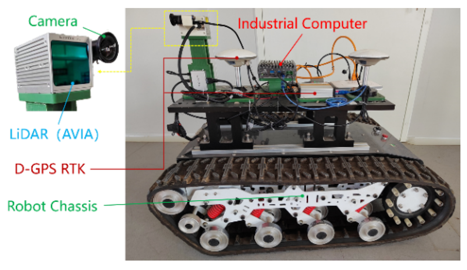
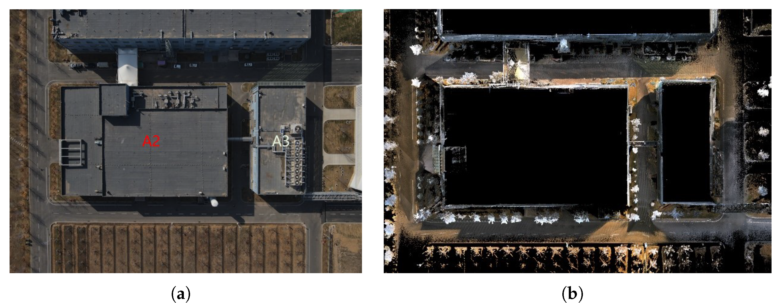
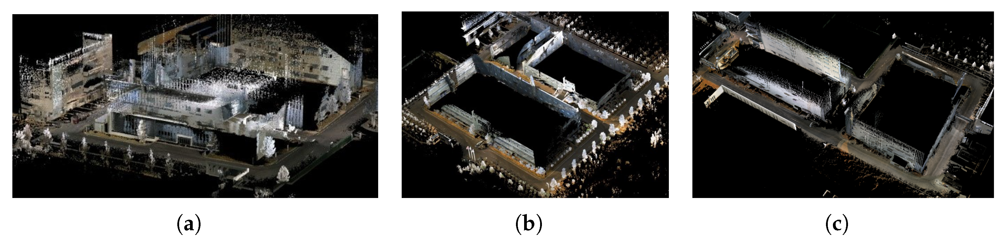
  • A variety of indoor and outdoor field experiments were conducted using a crawler robot (see Figure 1) to validate the robustness and accuracy of the system. Some field experiment results obtained are shown in Figure 2; regarding the roads surrounding the buildings, the algorithm proposed by us shows high accuracy in mapping, so it can meet the requirements of the navigation tasks of mobile robots.

2. Framework Overview

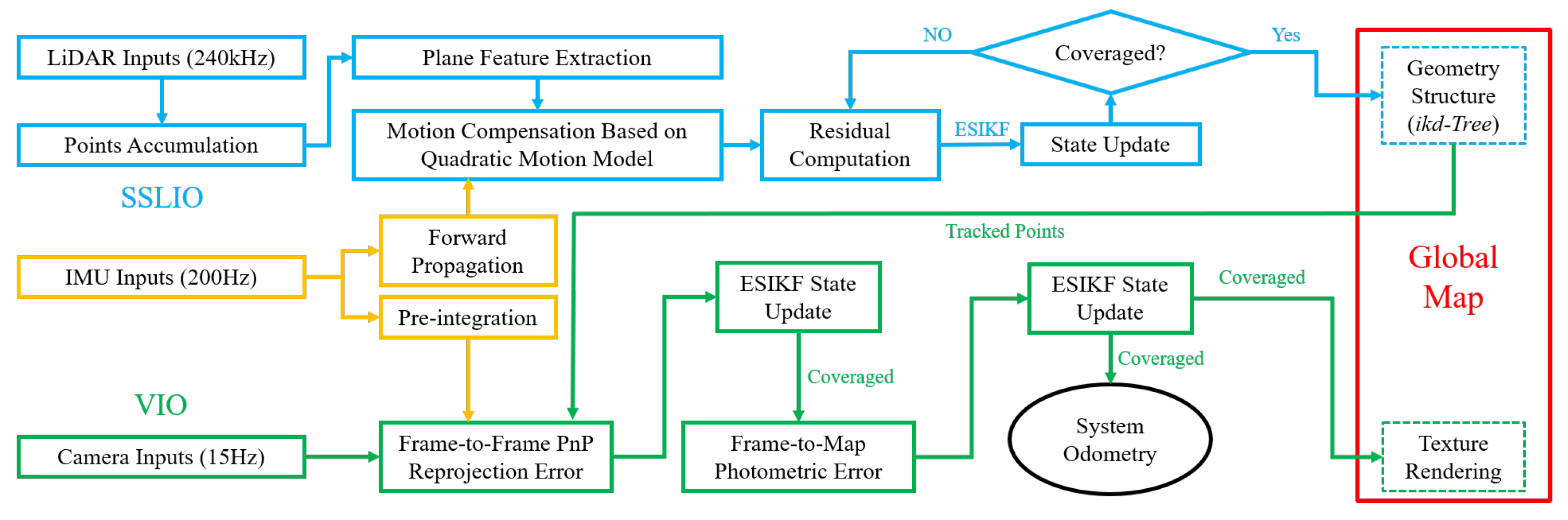
2.1. System Pipeline

Figure 3 provides an overview of our system pipeline. The SSLIO subsystem extracts the plane feature points from the accumulated LiDAR raw points, then performs the motion distortion compensation on the feature points based on the backward propagation of the quadratic motion model, and finally calculates the residuals and updates the subsystem state by ESIKF. The LiDAR feature points are transformed into the global frame to form the global map geometry structure represented by the ikd-Tree.
The VIO subsystem first selects the tracking points from the global map geometry structure to calculate the frame-to-frame PnP re-projection error and then uses ESIKF to perform the first update of the VIO subsystem state; then, it calculates the frame-to-map photometric error and uses ESIKF to perform the second state update, at which time the VIO subsystem state is used as the odometry output of the whole system. The obtained optimal state and state covariance are used for (1) global map RGB coloring (i.e., rendering the texture) and tracked points update, and (2) as the initial point for the forward propagation of the IMU in the subsequent scan of the SSLIO or IMU pre-integration in the next frame update of VIO. However, in order to improve the real-time performance of the system, unlike [25], which performs real-time estimation of the camera and IMU extrinsic parameter, our VIO calibrates this extrinsic parameter in advance. The detailed implementation procedure of our VIO subsystem can be found in [24,25].

2.2. Nomenclature and Full State Vector

Table 1 presents the key nomenclature used in this paper.
In this paper, the full-state variable is x defined as
x = G R I T G p I T G υ I T b g T b a T G g T I t C T M = S O ( 3 ) × R 16
where the dimension of the state manifold space M is dim M = 19 . The initial IMU body frame I is used as the reference global frame G. In Equation (1), G R I and G p I denote the rotation matrix and translation vector of the IMU with regard to the global frame, respectively; G g and G υ I are the acceleration of gravity and IMU velocity with regard to the global frame, respectively; and b a and b g are the biases of the accelerometer and gyroscope, respectively, for which the mathematical treatment is detailed in [28]. I t C represents the temporal difference between the timestamps of the camera data and IMU data. It plays a crucial role in the computation of the real-time time calibration factor within the VIO subsystem [30].

2.3. Extrinsic Calibration between Sensors

It is assumed that the exact extrinsic parameter I T L between the solid-state LiDAR and the IMU is known, and the camera and the solid-state LiDAR are rigidly connected together by a fixture. The exact extrinsic parameter L T C between the camera and the LiDAR is first obtained using the targetless calibration method [31], and then the extrinsic parameter I T C between the camera and the IMU can be calculated by the following transformation equation:
I T C = I R C , I p C = I T L L T C

3. Solid-State-LiDAR-Inertial Odometry Subsystem

The state update acquired upon the convergence of the ESIKF within the VIO subsystem serves as the most recent state of the entire system. This updated state is then employed as the initial point for the forward propagation of the IMU data in the subsequent scan of the SSLIO subsystem state update.
Our SSLIO subsystem is similar to Point-LIO, and the state estimation method is the tightly coupled error-state iterated Kalman filter. However, our SSLIO has two key novelties: (1) Unlike Point-LIO, which uses a point-by-point framework (i.e., the system state is updated once for each point measured by the LiDAR), our proposed SSLIO framework accumulates LiDAR points into one frame before processing (i.e., the state is updated frame by frame). Furthermore, it employs a quadratic motion model to handle the distortion of LiDAR point clouds caused by motion. (2) To exploit the high resolution of solid-state LiDAR, we designed a metric weighting function for the feature point residual term when constructing the LiDAR measurement model, which ensures both geometric consistency in feature correlation, like Point-LIO, and reflectivity consistency [19]. We assume that the extrinsic parameter is known. In fact, for rigidly connected LiDAR and IMU, their precise extrinsic parameter can be calibrated beforehand [32], while some manufacturers have produced a LiDAR with a built-in IMU (e.g., AVIA and MID-360 produced by LIVOX), whose precise extrinsic parameter is detailed in the product specifications.
Unlike most researchers’ derivation of the error-state Kalman filter on European space, such as in [33], to make our algorithm more suitable for mobile robot system, we use the ⊞ (“boxplus”) operation and its inverse ⊟ (“boxminus”) from [16,34] to parameterize the error-state on the n-dimensional differentiable manifold M :
: M × R n M ; : M × M R n S O 3 : R r = R Exp r ; R 1 R 2 = Log R 2 T R 1 R n : c d = c + d ; c d = c d
where Exp · and Log · denote the exponential map and logarithmic map on S O 3 , respectively, which are essentially Rodrigues’ transformations. Detailed definitions of ⊞ and ⊟ can be found in [34].

3.1. IMU State Transition Model

Since the SSLIO subsystem does not need to consider camera data, the state x represented by Equation (1) does not need to include the temporal difference I t C ; that is, the state x in the SSLIO subsystem is simplified as shown below:
x = G R I T G p I T G υ I T b g T b a T G g T T M = S O ( 3 ) × R 15
Moreover, the corresponding dimension of the differentiable manifold space M is dim M = 18 .
The standard IMU continuous-time kinematic model (see [33] for a detailed derivation) is
G R ˙ I = G R I ω m b g n g × G υ ˙ I = G R I a m b a n a + G g b ˙ g = n bg , b ˙ a = n ba
where a m and ω m are the measurements of the accelerometer and gyroscope, n a and n g denote the noise during the measurement, n ba and n bg are Gaussian noise, and for the definition of the symbol · × , the reader can refer to [28]. The derivatives of G g and G p I are 0 and G υ I , respectively.
To accommodate the discrete time interval Δ T (i.e., the time interval between two adjacent IMU measurements, denoted as Δ T ), the continuous-time kinematic model represented by Equation (4) can be transformed into a discrete-time kinematic model [34]:
x i + 1 = x i Δ T F x i , u i , w i
where x i denotes the state variable x at the moment τ i , function F can be seen in [13], and the input vector u and the process noise w are defined in [34].

3.2. Preprocessing of Raw LiDAR Points and Forward Propagation

The AVIA solid-state LiDAR samples roughly 240 k LiDAR points per second, and its built-in IMU takes 200 measurements per second, i.e., 240 kHz and 200 Hz for the LiDAR and IMU, respectively. The data obtained by the conventional mechanical spinning LiDAR for each 360 scan are called a scan (or a frame), but for the AVIA LiDAR, a scan needs to be defined artificially. In this paper, LiDAR points collected within 100 ms are defined as a scan so that LiDAR raw points and IMU measurements can be packaged and sent to an SSLIO subsystem at a frequency of 10 Hz for fusion.
As shown in Figure 4a, t k denotes the end moment of the k-th solid-state LiDAR scan, τ i denotes the i-th sampling moment of IMU during a solid-state LiDAR scan, and ρ j denotes the sampling moment of the j-th LiDAR feature point during a solid-state LiDAR scan. The raw points accumulated by the LiDAR during t k 1 , t k are called a LiDAR scan, and feature extraction is carried out on the raw points within a scan. As shown in Figure 4b, for all feature points extracted in a scan, plane feature points far outnumber edge feature points. To ensure the robustness of the subsequent state estimation, we only select plane feature points [35]. Please refer to [10] for detailed steps of the feature extraction. It is assumed that the number of feature points extracted during t k 1 , t k is m, and each feature point sampled at time ρ j is denoted as L j p f j ( L j denotes the local frame of the solid-state LiDAR at moment ρ j ). Note the sampling time of the m-th feature point ρ m = t k (i.e., the last feature point). There are multiple IMU measurements during t k 1 , t k , and each IMU measurement is sampled at τ i with the state x i as in Equation (3).
As shown in Figure 4a, the optimal state and covariance matrix of the whole system are assumed to be x ¯ k 1 * and ¯ k 1 * at t k 1 , respectively, by fusing the most recent LiDAR scan and the last frame image. Once the system receives a new IMU measurement input, it initiates the forward propagation process. In this process, the value of w i is set to 0 . Based on Equation (5), the forward propagation is
x ^ i + 1 = x ^ i Δ T F x ^ i , u i , w i ^ i + 1 = F x ˜ i ^ i F x ˜ i T + F w i Φ i F w i T
where Φ i is the covariance matrix of w i , and the calculation of the Jacobian matrix F x ˜ i and F w i can be referred to in the appendix of [13]. At the beginning of the forward propagation, x ^ 0 = x ¯ k 1 * , ^ 0 = ¯ k 1 * ; at the end of forward propagation (i.e., the end of the new k-th scan at t k ), the state propagation is x ^ k ( x k denotes the state variable x at the moment of t k ), and the covariance matrix is ^ k .

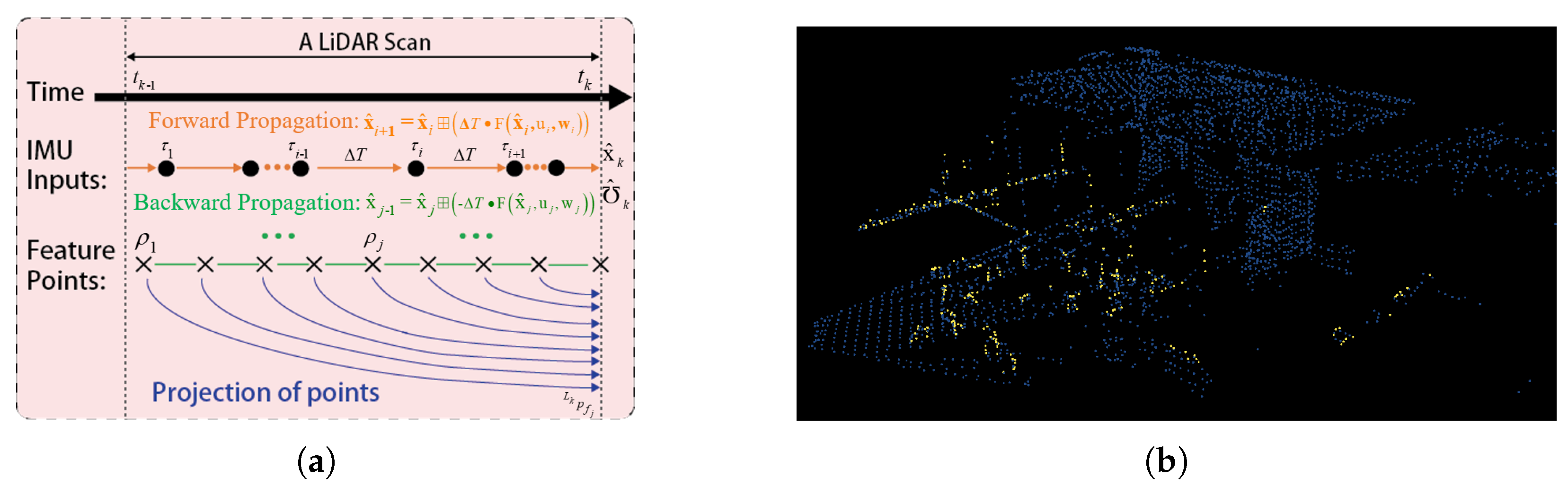
3.3. Motion Distortion Compensation Based on the Quadratic Motion Model

The difference between the LiDAR point sampling frequency and the IMU measurement frequency is huge; when performing in-frame (or in-scan) motion distortion compensation [36], if the angular velocity and acceleration between two adjacent IMU measurement are assumed to be constant (i.e., constant model), this assumption will be inappropriate to deal with in-frame motion distortion when facing situations such as drastic acceleration and angular velocity changes. To enable our SSLIO subsystem to cope with severe in-frame motion distortion, inspired by [23], we innovatively propose the quadratic motion model; that is, we fit the acceleration and angular velocity at any moment between two adjacent IMU measurements by a second-order polynomial depicting this variable motion:
ω = ζ 0 + ζ 1 Δ t ˙ + ζ 2 Δ t ˙ 2 , a = ϑ 0 + ϑ 1 Δ t ˙ + ϑ 2 Δ t ˙ 2
where Δ t ˙ is the time difference of ρ j from the right IMU measurement (the right measurement in two adjacent IMU measurements; that is, for ρ j τ i 1 , τ i , Δ t ˙ is the time difference between ρ j and τ i ). Compared to the constant model, the quadratic motion model adds first-order and second-order terms, and ζ α , ϑ α ( α = 0 , 1 , 2 ) is the coefficient being estimated.
Assuming that a series of data obtained by IMU measurements is available, the acceleration can be written as a η , a η 1 , a η + 1 , the angular velocity can be written as ω η , ω η 1 , ω η + 1 , and the subscript η denotes the discrete series. According to Equation (7), we have
1 Δ t ˙ 1 Δ t ˙ 1 2 1 0 0 1 Δ t ˙ 2 Δ t ˙ 2 2 ζ 0 ζ 1 ζ 2 = ω η 1 ω η ω η + 1 , 1 Δ t ˙ 1 Δ t ˙ 1 2 1 0 0 1 Δ t ˙ 2 Δ t ˙ 2 2 ϑ 0 ϑ 1 ϑ 2 = a η 1 a η a η + 1
where Δ t ˙ 1 = t η 1 t η , Δ t ˙ 2 = t η + 1 t η , t η 1 , t η and t η + 1 are the corresponding IMU measurement sample times; for example, you can take τ i 1 , τ i and τ i + 1 respectively, and the specific setting method can be determined according to the IMU frequency. Our quadratic motion model is essentially an interpolation method. As shown in Figure 4a, when interpolating the acceleration and angular velocity of ρ j at any moment in any interval τ i 1 , τ i during the period t k 1 , t k , our motion model takes into account the effect of the change of acceleration and angular velocity in the previous interval on it. Therefore, when our motion model interpolates the acceleration and angular velocity of ρ j at any moment in any interval τ i , τ i + 1 during the period t k 1 , t k , we uniformly use the data of the moments τ i 1 , τ i and τ i + 1 . Equation (8) can be simplified as
Γ Ω = ω , Γ = a
where Γ = 1 Δ t ˙ 1 Δ t ˙ 1 2 1 0 0 1 Δ t ˙ 2 Δ t ˙ 2 2 , Ω = ζ 0 ζ 1 ζ 2 , ω = ω η 1 ω η ω η + 1 , = ϑ 0 ϑ 1 ϑ 2 , a = a η 1 a η a η + 1 .
Using the generalized invertible matrix, we can estimate the coefficient vector as
Ω ^ = Γ T Γ 1 Γ T ω , ^ = Γ T Γ 1 Γ T a
where Γ T is the transpose of matrix Γ , Ω ^ = ζ ^ 0 ζ ^ 1 ζ ^ 2 T , ^ = ϑ ^ 0 ϑ ^ 1 ϑ ^ 2 T .
Substituting the estimated results Ω ^ and ^ into Equation (7), the angular velocity ω ^ and acceleration a ^ at any moment ρ j between the two adjacent IMU measurements can be obtained as given below:
ω ^ = ζ ^ 0 + ζ ^ 1 Δ t ˙ + ζ ^ 2 Δ t ˙ 2 , a ^ = ϑ ^ 0 + ϑ ^ 1 Δ t ˙ + ϑ ^ 2 Δ t ˙ 2
To eliminate the feature point motion distortion within the new scan and compensate for the relative motion between ρ j and t k , we use backward propagation (i.e., x ^ j 1 = x ^ j Δ T F x ^ j , u j , w j , x j denotes the state variable x at the moment of ρ j ) to obtain the pose of the body frame at feature points sampling moment ρ j relative to t k : I k T I j ( I j and I k denote the IMU body frame at the ρ j and t k , respectively). This relative pose converts the coordinate value L j p f j of the sampled points under the LiDAR local frame L j at the respective sampling moment ρ j to the coordinate value L k p f j under the LiDAR local frame L k at the end moment t k of the scan (see Figure 4a). For all feature points collected at the ρ j moment ( ρ j τ i 1 , τ i ) between two adjacent IMU measurements, we now have the measurement a m i 1 , ω m i 1 and the estimation a ^ , ω ^ at ρ j obtained from Equation (11). We can now take their average value as the backward propagation input, as given below:
a i 1 i n p u t = a m i 1 + a ^ 2 = a m i 1 + ϑ ^ 0 + ϑ ^ 1 Δ t ˙ + ϑ ^ 2 Δ t ˙ 2 2 ω i 1 i n p u t = ω m i 1 + ω ^ 2 = ω m i 1 + ζ ^ 0 + ζ ^ 1 Δ t ˙ + ζ ^ 2 Δ t ˙ 2 2
During the IMU backward propagation, the estimation x j of x j in relation to x k is as follows:
I k p I j 1 = I k p I j I k υ I j Δ t , s t a r t i n g f r o m I k p I m = 0 ; I k υ I j 1 = I k υ I j I k R I j ( a i 1 i n p u t b ^ a k ) Δ t I k g ^ k Δ t , s t a r t i n g f r o m I k υ I m = G R ^ I k T G υ I k , I k g ^ k = G R ^ I k T G g ^ k ; I k R I j 1 = I k R I j Exp ( ( b ^ g k ω i 1 i n p u t ) Δ t ) , s t a r t i n g f r o m I k R I m = I
where I k R I j and I k p I j are the rotation matrix and translation vector of I k T I j , respectively, and the Exp · operation rules refer to [16,34].
The transformation of L j p f j by the relative pose I k T I j is obtained from Equation (13) as given below:
L k p f j = I T L 1 I k T I j I T L L j p f j

3.4. Point-to-Plane Residual Computation

With the in-frame motion distortion removal in Equation (14), we treat all the plane feature points L k p f j within this new scan as being collected at t k . Assuming that the latest iteration of the SSLIO subsystem ESIKF is the γ -th one, the state estimation is x ^ k γ . When γ = 0, x ^ k γ = x ^ k , x ^ k is the predicted state obtained from the forward propagation Equation (6). When the measurement noise is not considered, we transform L k p f j to G: G p ^ f j γ ; j = 1 , , m . We search the global map for the five points p 1 j , p 2 j , p 3 j , p 4 j and p 5 j that are closest to the point G p ^ f j γ , which lie on the same tiny plane j . The measurement model is built using the distance between the global frame coordinate value G p ^ f j γ of the estimated feature point and the plane patch j (see concrete derivation in [16]):
0 = o j x k , L n j = G φ j T G T ^ I k γ I T L L k p f j + L n j G c j
where G φ j is the normal vector of the plane patch j , LiDAR measurement noise L n j is composed of ranging noise and beam-directing noise [31], G c j is the center of the plane patch j , and G T ^ I k γ is the pose of I relative to G at t k .
The measurement model represented by Equation (15) only considers the geometric consistency of the LiDAR feature points, and we designed a metric weighting function to ensure the reflectivity consistency:
ν j L j p f j = λ G φ j T G φ j exp ι = 1 5 r L j p f j r ι
where r L j p f j is the reflectivity (i.e., intensity) measured when the LiDAR acquires feature point L j p f j , r ι denotes the reflectivity of p ι j ( ι = 1 , 2 , 3 , 4 , 5 ), ν j L j p f j denotes the weight, and λ is a constant experience value. Combining Equations (15) and (16), we obtain the new measurement model as given below:
0 = o j x k , L n j = ν j L j p f j G φ j T G T ^ I k γ I T L L k p f j + L n j G c j
The approximate form of the measurement model (17) can be obtained by first-order approximation at x ^ k γ :
0 = o j x k , L n j o j x ^ k γ , 0 + O j γ x ˜ k γ + r j = Z j γ + O j γ x ˜ k γ + r j
where error-state x ˜ k γ = x k x ^ k γ (or equivalently x k = x ^ k γ x ˜ k γ ), and O j γ is the Jacobian matrix, i.e., the partial differential of o j in Equation (17) with respect to x ˜ k γ . The Z j γ shown below is the point-to-plane residual used to construct the maximum a posteriori estimation (MAP) problem:
Z j γ = o j x ^ k γ , 0 = ν j L j p f j G φ j T G T ^ I k γ I T L L k p f j G c j
Moreover, owing to the LiDAR raw measurement noise L n j , a total measurement noise r j = ν j L j p f j G φ j T G T ^ I k γ I T L L n j N 0 , j with covariance j is obtained. In the practical robot application, we set j to a constant value according to the specific operating environment of the robot, and the effect is excellent.

3.5. ESIKF Update

The prior distribution of error-state is as follows:
x k x ^ k = x ^ k γ x ˜ k γ x ^ k = x ^ k γ x ^ k + J γ x ˜ k γ N 0 , ^ k
where J γ is the Jacobian matrix of x k x ^ k with respect to x ^ k γ at 0 . Refer to [14] for calculation of J γ .
The observation distribution of error-state can be obtained from the measurement model (18) given below:
r j = Z j γ + O j γ x ˜ k γ N 0 , j
The MAP problem of x ˜ k γ is obtained by combining Equations (20) and (21) as given below:
min x ˜ k γ x k x ^ k ^ k 2 + j = 1 m Z j γ + O j γ x ˜ k γ j 2
Similarly to [16], the IKFoM [34] framework is used to solve the MAP problem, and the optimal x ¯ k and ¯ k of the SSLIO subsystem can be obtained. We use state update x ¯ k to transform the LiDAR plane feature points to G: G p ¯ j = G T ¯ I k γ I T L L k p f j ; j = 1 , , m . The points G p ¯ j that are appended to the global map eventually form the geometry structure of the global map.

4. Field Experiments and Evaluation Results

We used the Point-LIO publicly available dataset (available online https://github.com/hku-mars/Point-LIO (accessed on 5 July 2023)) and our own dataset for experiments.

4.1. Experimental Platform

To gather real-world data, we engineered a hardware system comprising a crawler robot and a sensor suite as depicted in Figure 1. The sensor suite consists of an AVIA LiDAR, AVIA, a HIKVISION MV-CA013-A0UC global shutter camera, a high-precision GNSS real-time kinematic (GNSS RTK) system, and an industrial computer. The AVIA LiDAR incorporates a BMI088 IMU and features an elliptical FoV measuring 70.4° (horizontal) × 77.2° (vertical). For target objects with 80% reflectivity and at 20 m away, the random error of LiDAR range is less than 2 cm and the random error of angle is less than 0.05 degrees. The BMI088 model IMU has an accelerometer and gyroscope with zero offset of ±20 mg and ±1 degree/s, respectively. The camera is equipped with a lens with an FoV of 82.9° (horizontal) × 66.5° (vertical). The GNSS RTK system was used to provide the reference ground-truth for our algorithm for quantitative evaluation. The industrial computer used for data collection is equipped with an ARM rev0(v8l)×6 CPU and 8 GB RAM.

4.2. Extrinsic Calibration between Camera and IMU

We used the targetless calibration method [31] to obtain the extrinsic calibration L T C = L R C , L p C between AVIA LiDAR and the HIKVISION camera. The basic idea of this calibration method is to extract natural edge features from a natural scene image (see Figure 5a) and corresponding scene LiDAR point cloud (see Figure 5b), and then match and align the edge features obtained by these two sensors. The maximum likelihood estimation equation of the extrinsic calibration L T C estimation was established, and then the estimation problem was solved iteratively. The LiDAR point cloud was projected onto the camera image using the initial extrinsic parameter before calibration and the optimal extrinsic parameter after calibration; the obtained calibration results can be evaluated. Figure 5c,d depict the LiDAR point cloud projection in the upper layer, while the lower layer illustrates the camera-captured image. From the red boxes marked in Figure 5c,d, evidently, it is observable that the initial extrinsic cannot make the LiDAR point cloud projection and image match well before calibration, while the calibrated extrinsic enables the projection and image to match well, indicating that the calibration results are accurate. After we obtained the exact L T C , the I T C could be calculated using Equation (2).

4.3. Experiment-1: Experimental Verification of the Validity of Quadratic Motion Model and Weight Function

To verify the effectiveness of the quadratic motion model and weight function in our SSLIO subsystem, we turned off the VIO subsystem and the global map RGB coloring function of our algorithm, and then conducted experiments using the public dataset and our private datasets.

4.3.1. Experiment-1.1: Public Dataset Experiment

To verify the robustness of the SSLIO subsystem at a high angular velocity, we used the “spinning_ platform” sequence from the Point-LIO public dataset to build a map. The “spinning_ platform” sequence collected data with AVIA fixed on a rotating platform, and the duration of the sequence was 130 s. In the first 40 s, the angular velocity of the rotating platform around the z-axis increased from 0 to 35 rad/s (35 rad/s is the angular velocity measurement limit of the built-in IMU of AVIA). Because our SSLIO subsystem is a tightly coupled LIO, we discarded the data collected during the last 90 s of the sequence, and used only the first 40 s of the sequence (because the actual angular velocity exceeded the built-in IMU angular velocity range of 35 rad/s for a long time in the last 90 s). Even if the angular velocity exceeded 30 rad/s, the map geometry built by our SSLIO subsystem basically reflects the real experimental environment as shown in Figure 6 (see [16] for the specific dataset acquisition environment).

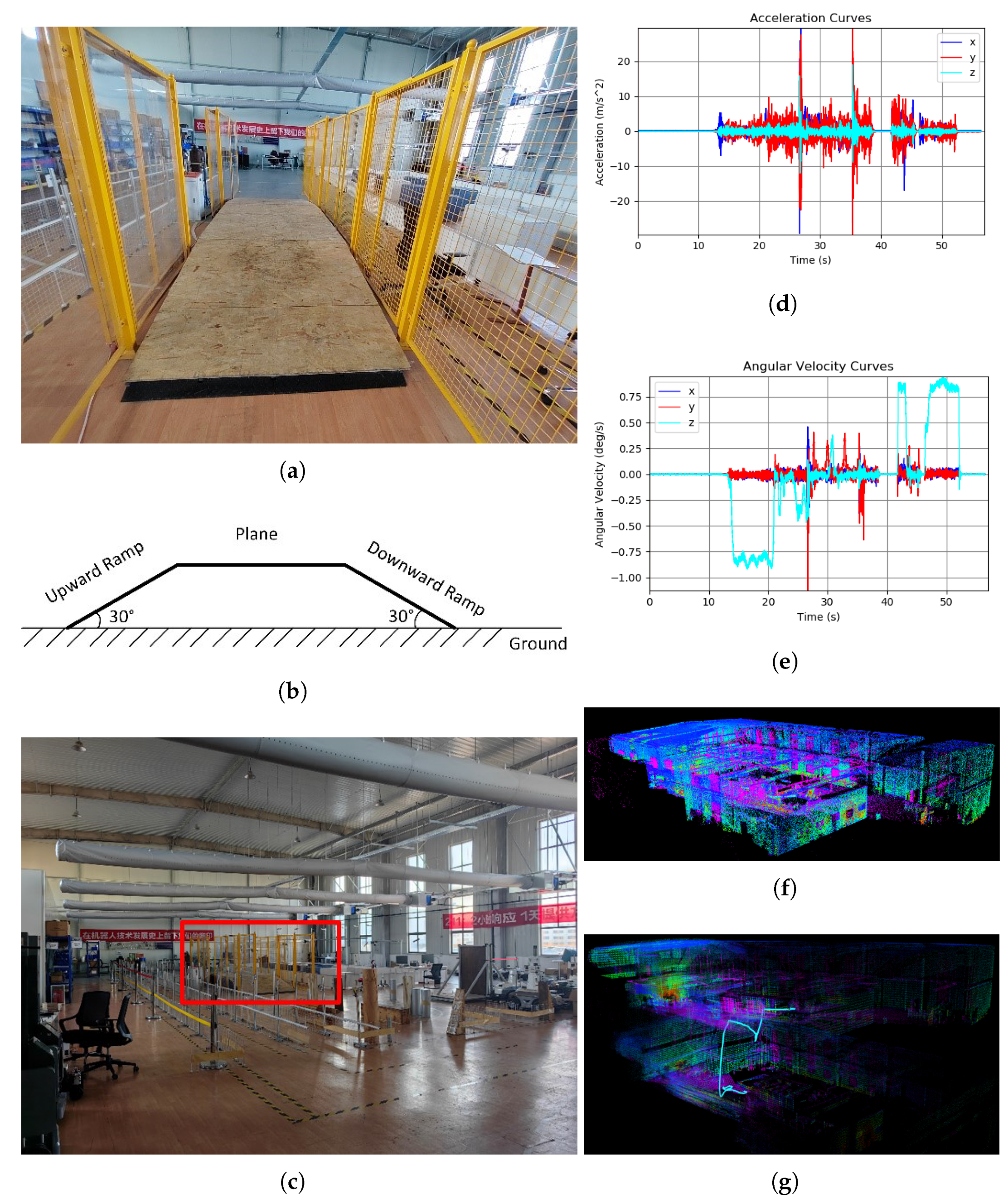
4.3.2. Experiment-1.2: Fast Crossing of the Steep Ramp Experiment Test

Motion distortion compensation based on the quadratic motion model helps the algorithm handle motion distortion, so we conducted a steep ramp experiment to verify the ability of the SSLIO subsystem to handle severe motion distortion. As shown in Figure 7a,b, the steep ramp test platform consists of an upward ramp, a plane, and a downward ramp, and it is located in a spacious plant with only one floor (as shown in the Figure 7c, the red box marks the location of the steep ramp).
During the experiment, the crawler robot first rotated in the ground, quickly rushed through the steep ramp test platform, and finally rotated in the ground. When the robot was moving fast on the steep ramp test platform, it would generate strong vibration. Owing to the absence of dampers, the vibration originating from the crawler robot chassis was directly transferred to the sensor suite, resulting in significant shaking. Figure 7d,e, exhibit the IMU measurements, revealing significant variations in both the acceleration and angular velocity (we suspect that the actual instantaneous acceleration maximum may have exceeded the measurement range of the IMU, i.e., 30 m/s2, but we lack equipment with a larger range to measure the actual maximum acceleration). Our proposed SSLIO subsystem and Point-LIO mapping results are shown in Figure 7f,g, respectively. The map generated by Point-LIO has a serious drift, and the plant that has only one floor becomes a plant with two floors in the map, while the mapping accuracy of our SSLIO for this plant is much better than that of Point-LIO.
In order to objectively illustrate that our proposed quadratic motion model has practical engineering utility, the dataset collected in the above-mentioned steep ramp experiment test was used to conduct mapping experiments in two cases: without quadratic motion model in SSLIO subsystem (called SSLIO-WQMM) and with piecewise linear model in SSLIO subsystem (called SSLIO-PLM) [37,38], respectively. The duration of the aforementioned collected steep ramp experiment test dataset totaled 56 s. As shown in Figure 8a, the SSLIO subsystem without quadratic motion model has serious drift in the odometry output and mapping results. The pose estimation and mapping of the whole subsystem starts to drift around the 25th second (when the acceleration and angular velocity start to change drastically), and the direction of drift is shown by the red arrows, and even the final estimated odometry trajectory is far beyond the area shown in the figure, which does not match with the actual motion trajectory of the crawler robot. The acceleration and angular velocity between the two adjacent IMU measurements are interpolated using a simple piecewise linear model and used in the backward propagation of SSLIO, called SSLIO, using a piecewise linear model, i.e., SSLIO-PLM. The final mapping result of this approach is shown in Figure 8b. Although the mapping result is much better compared to that of the SSLIO subsystem without a quadratic motion model, there is still a drift downward compared to the actual environment, such as the area marked by the red box, and such a mapping result will have an adverse effect on the robot’s subsequent tasks, such as path planning.
The experimental findings demonstrate that our quadratic motion model handles the motion distortion well, even when the acceleration and angular velocity vary drastically within a sample interval of the IMU.

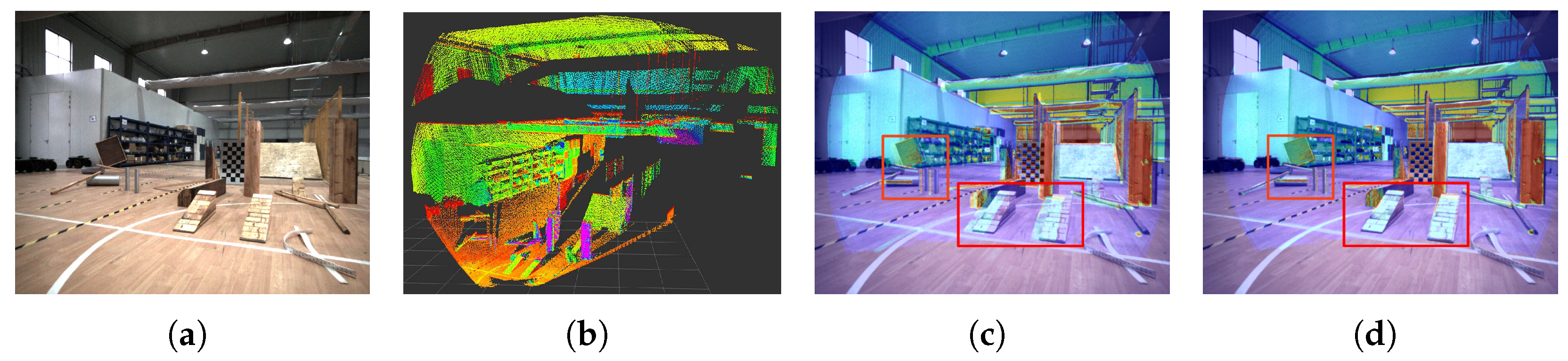
4.3.3. Experiment-1.3: Validation Experiment on the Validity of Weighting Function

To verify that the weight function designed by our algorithm can improve the construction accuracy of the global map geometry, we used the data collected between buildings B1 and B3 within Raytron (called B1B3_seq) for the validation experiments. During the acquisition of the B1B3_seq sequence, the crawler robot occasionally passed through a speed bump on the road, thus generating instantaneous and dramatic changes in acceleration. The maps were constructed using our proposed complete SSLIO subsystem and the SSLIO subsystem with the weight function omitted (called SSLIO-WFO), respectively. Figure 9a shows the SSLIO subsystem mapping result, and the mapping results are consistent with the data collection environment. In terms of mapping details, the experimental results indicate that SSLIO outperforms SSLIO-WFO in terms of accuracy. For example, for the small area marked by red box in Figure 9a, SSLIO-WFO mapping result is shown in Figure 9b, there is an extra wall that does not exist in the actual scene, and the actual scene taken by drone is shown in Figure 9c; the SSLIO mapping result for this area is shown in Figure 9d. The experimental results show that the weight function we designed makes a positive contribution to the map accuracy improvement.

4.4. Experiment-2: Quantitative Evaluation of Localization Accuracy Using GNSS RTK

By conducting a trajectory comparison between our proposed algorithm, VINS-Mono [28], and LiLiOM [19] against the ground-truth trajectory acquired through the GNSS RTK system, we were able to assess the quantitative accuracy of each algorithm. The trajectories were projected onto the Y-X plane as depicted in Figure 10. The difference between VINS-Mono and the ground-truth trajectory is large, and the LiLiOM trajectory and the trajectory of our system match the ground-truth trajectory fairly well. However, the length of the LiLiOM trajectory differs more from the ground-truth trajectory than our proposed algorithm (the length of the trajectory of each algorithm is shown in Table 2). Table 2 presents the root mean square error (RMSE) of the absolute pose error (APE) for the rotation angle, measured in radians (rad). Moreover, the rotation error of our proposed algorithm framework is smaller. The VINS-Mono trajectory is too different to have a reference for its rotation error, so it is not listed.

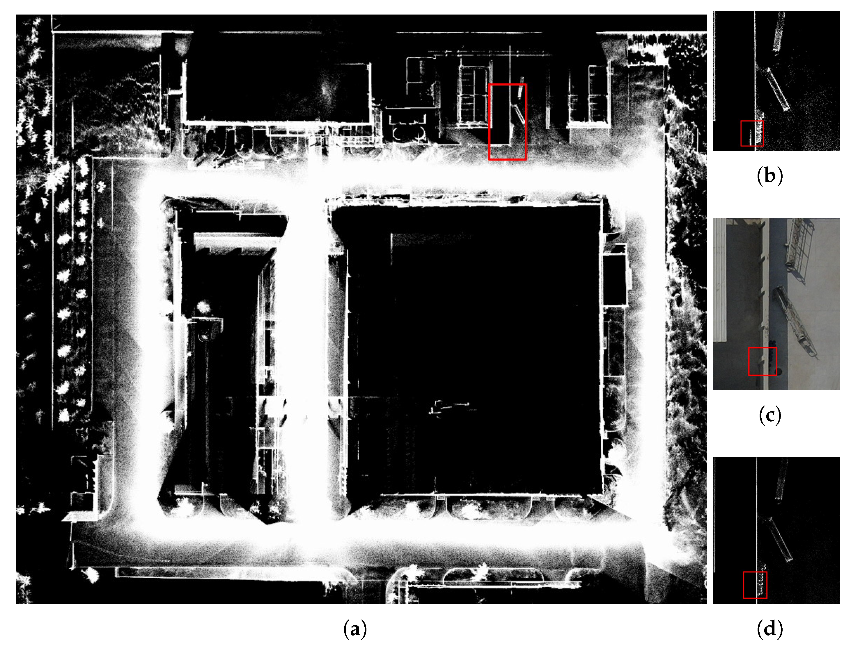
4.5. Experiment-3: Outdoor Large-Scale Challenging Factory Environment Mapping

This experiment collected multiple sequence datasets (i.e., B1B3_seq, A1A2A3_seq, and B1B3B4_seq, respectively) within Raytron, where many building facades are composed of glass, and there are often circular pipes above the roads, making it challenging to localization and mapping [39]. The mapping of the three sequences is shown in Figure 11a–c. Our proposed algorithm can accurately reconstruct RGB-colored, 3D-dense, large-scene modern factory plant environments, and the maps can be used for outdoor robot navigation. However, when our proposed algorithm framework builds the map, RGB color distortion is easily seen for the tiny branches on the trees on both sides of the road, as shown in Figure 11b, where the originally yellowish branches turn white instead.
The APE of each sequence is shown in Figure 12a–c. Each sequence trajectory reference length and RMSE of APE with regard to the translational part is shown in Table 3, and the reference is provided by the GNSS RTK system.

4.6. Run-Time Analysis

The computing platform on which our algorithm runs is a desktop computer with an i9-11900 CPU and 48 GB RAM. We used the three sequences of data collected in Experiment-3 for the run-time analysis. Compared to the multi-sensor fusion algorithm R3LIVE, since our main difference and novelties are in the SSLIO subsystem, we compared the average time consumption of our SSLIO subsystem with that of the LIO subsystem of R3LIVE for processing each frame LiDAR point (as shown in Table 4). Our SSLIO subsystem takes longer than the LIO subsystem of R3LIVE because of the quadratic motion model in the motion compensation and the calculation of the residual term weight for each LiDAR feature point. However, our SSLIO subsystem still requires less than 100 ms per frame (i.e., cumulative time per LiDAR point frame), meeting the real-time requirement.

5. Discussion

Our solid-state-LiDAR-inertial-visual fusion system is divided into two modules: the SSLIO subsystem and the VIO subsystem. SSLIO utilizes the point clouds obtained from LiDAR scans to form the geometry of the global map, and VIO, in addition to further refining the state output obtained from SSLIO, will also color the global map. The results of the field experiments and evaluations illustrate that our proposed ESIKF-based multi-sensor fusion SLAM system can provide robust localization and mapping for robots in challenging situations. This section will delve into the practical engineering implications of our algorithm and its advantages over existing classical algorithms, explore different research paths, and elucidate the shortcomings of our system and directions for extended applications.
Our main innovation lies in the SSLIO subsystem, including the quadratic motion model and the weight function designed by utilizing the reflectivity information. Through the steep ramp experiment test, it is demonstrated that our proposed quadratic motion model not only can cope with drastic changes in acceleration and angular velocity more effectively than SSLIO-WQMM and SSLIO-PLM but also shows better motion compensation capability compared with the state-of-the-art solid-state LiDAR-inertial SLAM algorithm Point-LIO. This is of great significance when the robot performs real-world engineering tasks, such as rapidly crossing rocky hillsides and speed bumps on the ground, where the robot transmits vibrations to the IMU and causes drastic changes in acceleration and angular velocity measurements. The accumulation time of a frame of our LiDAR point cloud is 100 ms, while our SSLIO processes each frame in less than 30 ms on average, which greatly satisfies the real-time requirement.
In addition, in order to reduce the number of state components that need to be estimated during state estimation, we used an indirect approach to calibrate the extrinsic parameters of the VIO subsystem in advance.
In order to verify the robustness and accuracy of the whole system for localization in outdoor environments, we quantitatively evaluated our algorithm using a GNSS RTK device and compared it with the classical algorithms VINS-Mono and LiLiOM. The experimental results show that under the same environment, compared to VINS-Mono and LiLiOM, the robot trajectory estimated by our proposed algorithm not only matches the reference trajectory provided by the GNSS RTK equipment better but also has a smaller APE regarding the rotation.
However, our algorithm is prone to color distortion for objects such as small branches when mapping, and we still need to further improve our VIO coloring function.
In terms of SLAM, to further improve the robustness of our proposed algorithm in robot navigation tasks, we can incorporate loop closure detection, such as DBoW2 [40], intensity scan context [20], and STD [41]. To avoid the estimation of the temporal difference between IMU and camera data, we can employ hardware synchronization to synchronize the timestamps of the three sensors [26]. If further extended, our algorithm can be used for game development and VR [25].

6. Conclusions

This paper introduces a framework for odometry and mapping, utilizing an ESIKF, which integrates data from solid-state LiDAR, a camera, and IMU. We used the quadratic motion model in the motion compensation of the SSLIO subsystem; in addition, we designed a weight function for the LiDAR point residual term to ensure the geometric consistency and reflectivity consistency in feature association. To evaluate our work, after calibrating the extrinsic parameter between the camera and IMU, we carried out a public dataset experiment, a steep ramp experiment, localization accuracy quantitative evaluation experiments, outdoor large-scene modern factory plant mapping experiments, and run-time analysis in the field. The experimental results showed that (1) our tightly coupled SSLIO subsystem can handle instantaneous and drastic acceleration and angular velocity changes, and the accuracy of SSLIO can still meet the mapping requirements even when the acceleration and angular velocity reach 30 m/s2 and 35 rad/s, respectively. (2) High-performance localization and mapping are achieved by our proposed multi-sensor fusion SLAM framework, as well as its guaranteed real-time performance. However, our algorithm is prone to RGB color distortion when handling tiny cylindrical objects and therefore needs to be improved.

Author Contributions

Conceptualization, J.Y. and T.Y.; Methodology, T.Y. and J.Y.; Software, T.Y. and C.N.; Validation, T.Y., J.Y. and Y.L.; Formal Analysis, J.Y. and C.N.; Investigation, J.Y. and T.Y.; Resources, J.Y.; Data Curation, T.Y., Y.L. and C.N.; Writing—Original Draft Preparation, T.Y. and J.Y.; Writing—Review and Editing, J.Y. and T.Y.; Visualization, T.Y. and Y.L.; Supervision, J.Y. All authors have read and agreed to the published version of the manuscript.

Funding

This work was funded by the Shandong Province Key R&D Program of the Department of Science and Technology of Shandong Province (Research and Application of High-Efficiency Construction Technology for High-End Passenger Rolling Vessels, 2021CXGC010702 and Research and Application of Key Technology of Intelligent River and Sea Direct Access Vessel, 2022CXGC020403).

Institutional Review Board Statement

Our work does not involve any ethical guidelines.

Data Availability Statement

We used a dataset from Point-LIO, which is available online. We have to use the private experimental datasets collected in this paper for further research, so we did not make it publicly available.

Acknowledgments

The authors thank the Robotics and Artificial Intelligence Laboratory of Raytron for supporting the experiments of this paper, as well the master’s student Xiuxuan Qin of Yantai Research Institute at Harbin Engineering University for his help processing the experimental data.

Conflicts of Interest

The authors affirm that there are no potential conflicts of interest regarding the research, authorship, and publication of this article.

Abbreviations

The manuscript utilizes the following abbreviations:
SLAMSimultaneous localization and mapping
ESIKFError-state iterated Kalman filter
SSLIOSolid-state-LiDAR-inertial odometry
VIOVisual-inertial odometry

References

  1. Chen, N.; Kong, F.; Xu, W.; Cai, Y.; Li, H.; He, D.; Qin, Y.; Zhang, F. A self-rotating, single-actuated UAV with extended sensor field of view for autonomous navigation. Sci. Robot. 2023, 8, eade4538. [Google Scholar] [CrossRef] [PubMed]
  2. Chen, W.; Wang, Y.; Chen, H.; Liu, Y. EIL-SLAM: Depth-enhanced edge-based infrared-LiDAR SLAM. J. Field Robot. 2022, 39, 117–130. [Google Scholar] [CrossRef]
  3. Wang, J.; Chen, F.; Huang, Y.; McConnell, J.; Shan, T.; Englot, B. Virtual Maps for Autonomous Exploration of Cluttered Underwater Environments. IEEE J. Ocean. Eng. 2022, 47, 916–935. [Google Scholar] [CrossRef]
  4. Sousa, R.B.; Sobreira, H.M.; Moreira, A.P. A systematic literature review on long-term localization and mapping for mobile robots. J. Field Robot. 2023, 40, 1245–1322. [Google Scholar] [CrossRef]
  5. Chen, W.; Zhou, C.; Shang, G.; Wang, X.; Li, Z.; Xu, C.; Hu, K. SLAM Overview: From Single Sensor to Heterogeneous Fusion. Remote Sens. 2022, 14, 6033. [Google Scholar] [CrossRef]
  6. Elhashash, M.; Albanwan, H.; Qin, R. A Review of Mobile Mapping Systems: From Sensors to Applications. Sensors 2022, 22, 4262. [Google Scholar] [CrossRef] [PubMed]
  7. Lopac, N.; Jurdana, I.; Brnelić, A.; Krljan, T. Application of Laser Systems for Detection and Ranging in the Modern Road Transportation and Maritime Sector. Sensors 2022, 22, 5946. [Google Scholar] [CrossRef]
  8. Robosense Laser Beam Solid-State Lidar Priced At 1898. Available online: https://lidarnews.com/ (accessed on 15 June 2023).
  9. Van Nam, D.; Gon-Woo, K. Solid-State LiDAR based-SLAM: A Concise Review and Application. In Proceedings of the IEEE International Conference on Big Data and Smart Computing (BigComp), Jeju Island, Republic of Korea, 17–20 January 2021. [Google Scholar]
  10. Lin, J.; Zhang, F. Loam_ livox: A fast, robust, high-precision LiDAR odometry and mapping package for LiDARs of small FoV. In Proceedings of the IEEE International Conference on Robotics and Automation (ICRA), Paris, France, 31 May–15 June 2020. [Google Scholar]
  11. Yuan, C.; Xu, W.; Liu, X.; Hong, X.; Zhang, F. Efficient and Probabilistic Adaptive Voxel Mapping for Accurate Online LiDAR Odometry. IEEE Robot. Autom. Lett. 2022, 7, 8518–8525. [Google Scholar] [CrossRef]
  12. Wang, H.; Wang, C.; Xie, L.H. Lightweight 3-D Localization and Mapping for Solid-State LiDAR. IEEE Robot. Autom. Lett. 2021, 6, 1801–1807. [Google Scholar] [CrossRef]
  13. Xu, W.; Zhang, F. FAST-LIO: A Fast, Robust LiDAR-Inertial Odometry Package by Tightly-Coupled Iterated Kalman Filter. IEEE Robot. Autom. Lett. 2021, 6, 3317–3324. [Google Scholar] [CrossRef]
  14. Xu, W.; Cai, Y.; He, D.; Lin, J.; Zhang, F. FAST-LIO2: Fast Direct LiDAR-Inertial Odometry. IEEE Trans. Robot. 2022, 38, 2053–2073. [Google Scholar] [CrossRef]
  15. Cai, Y.; Xu, W.; Zhang, F. Ikd-tree: An incremental kd tree for robotic applications. arXiv 2021, arXiv:2102.10808. [Google Scholar]
  16. He, D.; Xu, W.; Chen, N.; Kong, F.; Yuan, C.; Zhang, F. Point-LIO: Robust High-Bandwidth Light Detection and Ranging Inertial Odometry. Adv. Intell. Syst. 2023. [Google Scholar] [CrossRef]
  17. Bai, C.; Xiao, T.; Chen, Y.; Wang, H.; Zhang, F.; Gao, X. Faster-LIO: Lightweight Tightly Coupled Lidar-Inertial odometry Using Parallel Sparse Incremental Voxels. IEEE Robot. Autom. Lett. 2022, 7, 4861–4868. [Google Scholar] [CrossRef]
  18. Zhang, J.; Singh, S. LOAM: Lidar Odometry and Mapping in Real-time. In Proceedings of the 10th Robotics: Science and Systems, RSS 2014, Berkeley, CA, USA, 12–16 July 2014. [Google Scholar]
  19. Li, K.L.; Li, M.; Hanebeck, U.D. Towards High-Performance Solid-State-LiDAR-Inertial Odometry and Mapping. IEEE Robot. Autom. Lett. 2021, 6, 5167–5174. [Google Scholar] [CrossRef]
  20. Wang, H.; Wang, C.; Xie, L. Intensity Scan Context: Coding Intensity and Geometry Relations for Loop Closure Detection. In Proceedings of the IEEE International Conference on Robotics and Automation (ICRA), Paris, France, 31 May–15 June 2020. [Google Scholar]
  21. Zhang, Y.; Tian, Y.; Wang, W.; Yang, G.; Li, Z.; Jing, F.; Tan, M. RI-LIO: Reflectivity Image Assisted Tightly-Coupled LiDAR-Inertial Odometry. IEEE Robot. Autom. Lett. 2023, 8, 1802–1809. [Google Scholar] [CrossRef]
  22. Liu, K.; Ma, H.; Wang, Z. A Tightly Coupled LiDAR-IMU Odometry through Iterated Point-Level Undistortion. arXiv 2022, arXiv:2209.12249. [Google Scholar]
  23. Ma, X.; Yao, X.; Ding, L.; Zhu, T.; Yang, G. Variable Motion Model for Lidar Motion Distortion Correction. In Proceedings of the Conference on AOPC—Optical Sensing and Imaging Technology, Beijing, China, 20–22 June 2021. [Google Scholar]
  24. Lin, J.; Zheng, C.; Xu, W.; Zhang, F. R (2) LIVE: A Robust, Real-Time, LiDAR-Inertial-Visual Tightly-Coupled State Estimator and Mapping. IEEE Robot. Autom. Lett. 2021, 6, 7469–7476. [Google Scholar] [CrossRef]
  25. Lin, J.; Zhang, F. R3LIVE: A Robust, Real-time, RGB-colored, LiDAR-Inertial-Visual tightly-coupled state Estimation and mapping package. In Proceedings of the 39th IEEE International Conference on Robotics and Automation, Philadelphia, PA, USA, 23–27 May 2022. [Google Scholar]
  26. Zheng, C.; Zhu, Q.; Xu, W.; Liu, X.; Guo, Q.; Zhang, F. FAST-LIVO: Fast and Tightly-coupled Sparse-Direct LiDAR-Inertial-Visual Odometry. In Proceedings of the IEEE/RSJ International Conference on Intelligent Robots and Systems (IROS), Kyoto, Japan, 23–27 October 2022. [Google Scholar]
  27. Shan, T.; Englot, B.; Ratti, C.; Rus, D. LVI-SAM: Tightly-coupled Lidar-Visual-Inertial Odometry via Smoothing and Mapping. In Proceedings of the IEEE International Conference on Robotics and Automation (ICRA), Xi’an, China, 30 May–5 June 2021. [Google Scholar]
  28. Qin, T.; Li, P.L.; Shen, S.J. VINS-Mono: A Robust and Versatile Monocular Visual-Inertial State Estimator. IEEE Trans. Robot. 2018, 34, 1004–1020. [Google Scholar] [CrossRef]
  29. Shan, T.; Englot, B.; Meyers, D.; Wang, W.; Ratti, C.; Rus, D. LIO-SAM: Tightly-coupled Lidar Inertial Odometry via Smoothing and Mapping. In Proceedings of the IEEE/RSJ International Conference on Intelligent Robots and Systems (IROS), Las Vegas, NV, USA, 24 October–24 January 2020. [Google Scholar]
  30. Qin, T.; Shen, S.J. Online Temporal Calibration for Monocular Visual-Inertial Systems. In Proceedings of the 25th IEEE/RSJ International Conference on Intelligent Robots and Systems (IROS), Madrid, Spain, 1–5 October 2018. [Google Scholar]
  31. Yuan, C.; Liu, X.; Hong, X.; Zhang, F. Pixel-Level Extrinsic Self Calibration of High Resolution LiDAR and Camera in Targetless Environments. IEEE Robot. Autom. Lett. 2021, 6, 7517–7524. [Google Scholar] [CrossRef]
  32. Mishra, S.; Pandey, G.; Saripalli, S. Target-free Extrinsic Calibration of a 3D-Lidar and an IMU. In Proceedings of the IEEE International Conference on Multisensor Fusion and Integration for Intelligent Systems (MFI), Karlsruhe, Germany, 23–25 September 2021. [Google Scholar]
  33. Sola, J. Quaternion kinematics for the error-state Kalman filter. arXiv 2017, arXiv:1711.02508. [Google Scholar]
  34. He, D.; Xu, W.; Zhang, F. Kalman filters on differentiable manifolds. arXiv 2021, arXiv:2102.03804. [Google Scholar]
  35. Yuan, Z.; Lang, F.; Xu, T.; Yang, X. LIW-OAM: Lidar-Inertial-Wheel Odometry and Mapping. arXiv 2023, arXiv:2302.14298. [Google Scholar]
  36. Neuhaus, F.; Koc, T.; Kohnen, R.; Paulus, D. MC2SLAM: Real-Time Inertial Lidar Odometry Using Two-Scan Motion Compensation. In Proceedings of the 40th German Conference on Pattern Recognition, Stuttgart, Germany, 9–12 October 2018. [Google Scholar]
  37. Esfandiari, R.S. Numerical Methods for Engineers and Scientists Using MATLAB, 2nd ed.; CRC Press: Boca Raton, FL, USA, 2017; pp. 160–248. [Google Scholar]
  38. Rabbath, C.A.; Corriveau, D. A comparison of piecewise cubic Hermite interpolating polynomials, cubic splines and piecewise linear functions for the approximation of projectile aerodynamics. Def. Technol. 2019, 15, 741–757. [Google Scholar] [CrossRef]
  39. Tibebu, H.; Roche, J.; De Silva, V.; Kondoz, A. LiDAR-Based Glass Detection for Improved Occupancy Grid Mapping. Sensors 2021, 21, 2263. [Google Scholar] [CrossRef] [PubMed]
  40. Galvez-Lopez, D.; Tardos, J.D. Bags of Binary Words for Fast Place Recognition in Image Sequences. IEEE Trans. Robot. 2012, 28, 1188–1197. [Google Scholar] [CrossRef]
  41. Yuan, C.; Lin, J.; Zou, Z.; Hong, X.; Zhang, F. STD: Stable Triangle Descriptor for 3D place recognition. arXiv 2022, arXiv:2209.12435. [Google Scholar]
Figure 1. Experimental platform for validation. The hardware sensors consist of a LIVOX AVIA LiDAR, a monocular camera, an industrial computer, and a GNSS RTK system. The hardware sensors are carried by a crawler robot.
Electronics 12 03633 g001
Figure 2. An example of mapping around the A2 building and A3 building of Raytron Technology Co. (called Raytron). (a) the color image depicting the mapping region taken from a top view by a DJI Mavic3 drone; (b) the mapping result (top view) of the proposed algorithm.
Electronics 12 03633 g002
Figure 3. System pipeline of our proposed algorithm framework. The system is generally divided into the solid-state-LiDAR-inertial odometry (SSLIO) subsystem (the blue part) and visual-inertial odometry (VIO) subsystem (the green part).
Electronics 12 03633 g003
Figure 4. LiDAR measurement processing schematic. (a) IMU forward propagation and backward propagation; (b) extracted plane (blue) and edge (yellow) features.
Electronics 12 03633 g004
Figure 5. Extrinsic calibration between AVIA LiDAR and the HIKVISION camera. (a) natural scene image; (b) LiDAR point cloud; (c) before calibration; (d) after calibration.
Electronics 12 03633 g005
Figure 6. Mapping results of SSLIO subsystem using “spinning_ platform” sequence.
Electronics 12 03633 g006
Figure 7. Steep ramp experiment test. (a) steep ramp test platform (front view); (b) steep ramp test platform diagram (side view); (c) internal environment of the plant; (d) acceleration curves; (e) angular velocity curves; (f) our proposed SSLIO subsystem mapping results; (g) Point-LIO mapping results.
Electronics 12 03633 g007
Figure 8. Validation of effect of quadratic motion model. (a) The results of our SSLIO subsystem mapping without quadratic motion model; (b) the results of our SSLIO subsystem mapping when using a piecewise linear model.
Electronics 12 03633 g008
Figure 9. Weighting function validation experiment. (a) Mapping result of SSLIO subsystem using B1B3_seq; (b) small-area SSLIO-WFO mapping result; (c) small-area drone image; (d) small-area SSLIO mapping result.
Electronics 12 03633 g009
Figure 10. The comparison of trajectories in Experiment-2.
Electronics 12 03633 g010
Figure 11. The result of each sequence mapping. (a) B1B3_seq; (b) A1A2A3_seq; and (c) B1B3B4_seq.
Electronics 12 03633 g011
Figure 12. The result of each sequence APE. (a) B1B3_seq; (b) A1A2A3_seq; and (c) B1B3B4_seq.
Electronics 12 03633 g012
Table 1. Important nomenclature.
SymbolsMeanings
G · Component of the state in global frame.
L · Component of the state in LiDAR frame.
I T L Extrinsic for transformation between LiDAR frame to IMU frame(the extrinsic parameter T includes the rotation matrix R and the translation vector p , i.e., T = R , p , the same below).
I T C Extrinsic for transformation between camera frame to IMU frame.
x , x ^ , x ¯ Ground-truth state, propagation state, and ESIKF update state, respectively.
x ˜ Error-state (i.e., the difference between the ground-truth x and its corresponding estimation x ^ ).
Table 2. The comparison of trajectory length estimated by different algorithms.
Ground TruthProposedLiLiOMVINS-Mono
Length of851.671856.067882.4191136.503
trajectory (m)
Rotation error (rad)×0.01080.0380×
Table 3. The reference length of each sequence trajectory and APE.
B1B3_seqA1A2A3_seqB1B3B4_seq
Length of reference
trajectory (m)
586.931655.166709.091
RMSE (m)0.5241.4491.529
Table 4. SSLIO (or LIO) subsystem average time consumption per frame.
B1B3_seqA1A2A3_seqB1B3B4_seq
SSLIO per-frame
cost time (ms)
27.1526.9727.23
LIO per-frame
cost time (ms)
19.3519.9420.11
Disclaimer/Publisher’s Note: The statements, opinions and data contained in all publications are solely those of the individual author(s) and contributor(s) and not of MDPI and/or the editor(s). MDPI and/or the editor(s) disclaim responsibility for any injury to people or property resulting from any ideas, methods, instructions or products referred to in the content.

