BFD-YOLO: A YOLOv7-Based Detection Method for Building Façade Defects

Abstract

Façade defects not only detract from the building’s aesthetics but also compromise its performance. Furthermore, they potentially endanger pedestrians, occupants, and property. Existing deep-learning-based methodologies are facing some challenges in terms of recognition speed and model complexity. An improved YOLOv7 method, named BFD-YOLO, is proposed to ensure the accuracy and speed of building façade defects detection in this paper. Firstly, the original ELAN module in YOLOv7 was substituted with a lightweight MobileOne module to diminish the quantity of parameters and enhance the speed of inference. Secondly, the coordinate attention module was added to the model to enhance feature extraction capability. Next, the SCYLLA-IoU was used to expedite the rate of convergence and increase the recall of the model. Finally, we have extended the open datasets to construct a building façade damage dataset that includes three typical defects. BFD-YOLO demonstrates excellent accuracy and efficiency based on this dataset. Compared to YOLOv7, BFD-YOLO’s precision and [email protected] are improved by 2.2% and 2.9%, respectively, while maintaining comparable efficiency. The experimental results indicate that the proposed method obtained higher detection accuracy with guaranteed real-time performance.

1. Introduction

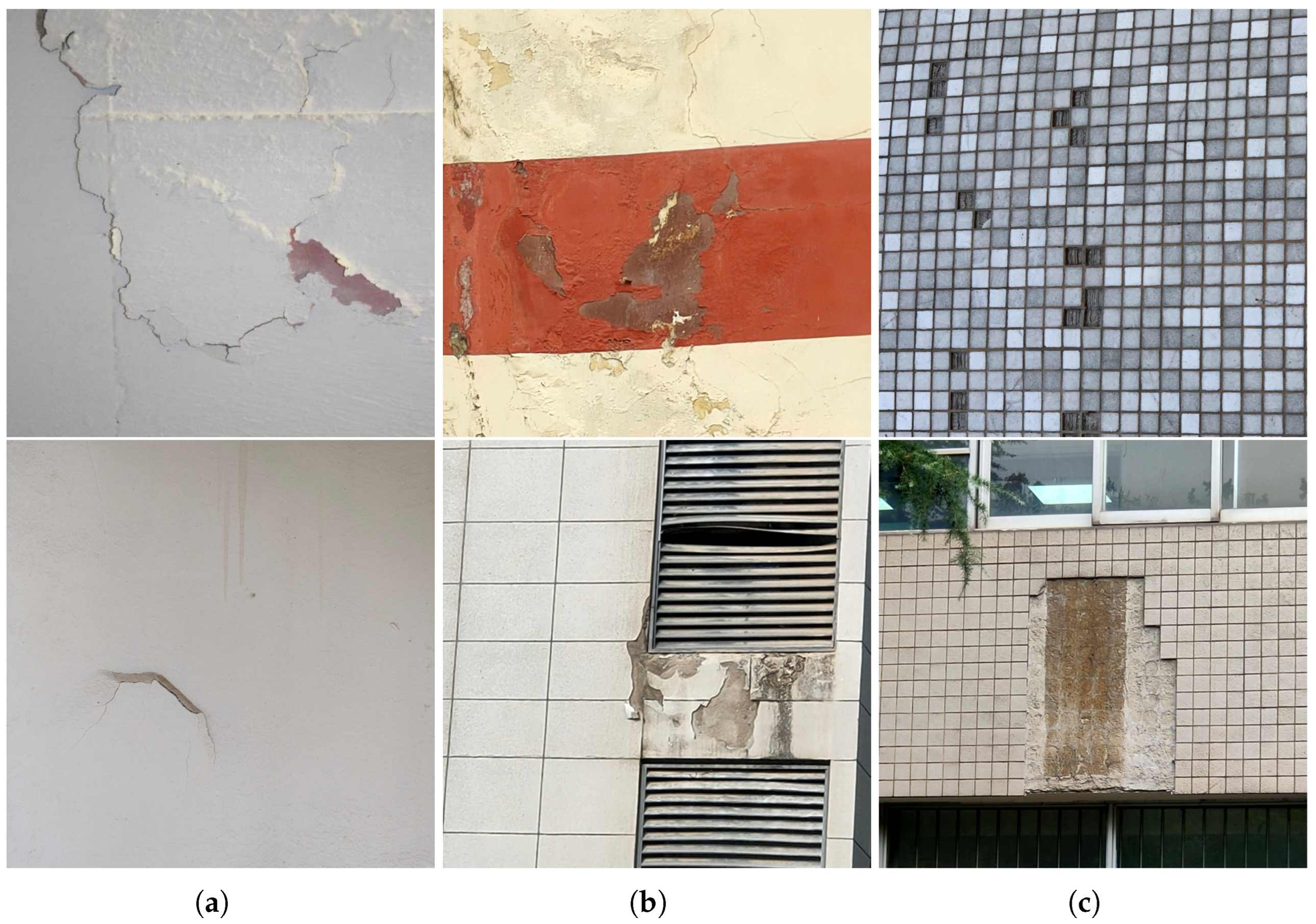
The presence of façade defects is a pressing issue in the operational phase of buildings, which is commonly attributed to mechanical and environmental factors. Typical defects manifest as concrete peeling, decorative spalling, component cracks, large-scale deformation, tile injury, moisture damage, etc. [1,2,3,4]. These defects can affect the appearance and reduce the service life expectancy of the building. More seriously, the façade falling objects may cause safety accidents and irreparable losses [5]. Structural damage detection is an integral part of structural health monitoring (SHM) and is essential for ensuring the safe operation of buildings [6]. As a component of structural damage detection, the detection of building façade defects can enable the government and management to gain a precise comprehension of the comprehensive status of the building façade, thereby facilitating the establishment of rational maintenance programs. It is an effective approach to reduce building maintenance costs, extend building service life, and mitigate the impact of façade damage [7]. Policies for regular standardized visual inspections are now being developed in many countries and regions [8,9]. The detection of building façade defects has become a critical component of building maintenance.

Visual inspection is an easy and trustworthy method to evaluate the condition of a building façade [10]. Conventional building façade inspection usually requires professionals with specialized tools to reach the inspection location, where visual observation, hammering, and other techniques are utilized for the assessment. These methods rely on the expertise and experience of the inspectors, which are subjective, dangerous, and inefficient [11]. Owing to the incremental quantity and growing size of buildings, manual visual inspection methods have become inadequate for fulfilling the demands of large-scale inspection. With the advancement of technology, many new methods (such as laser scanning, 3D thermal imaging, and SLAM) are being utilized for façade damage inspection via drones and robotic platforms [12]. These new methods are more convenient and safer compared with traditional techniques, but they are time-consuming and high-cost [13]. So, these methods are also confronting challenges in meeting the demands for large-scale inspections. Therefore, the development of a more precise and efficient method for detecting façade defects is necessary to enhance inspection efficiency and decrease computational costs [14].

Recent years have seen widespread adoption of deep learning in SHM, particularly in structural damage detection [15,16]. Object detection algorithms based on deep learning can be classified into two primary categories. One category is the two-stage region-proposal-based algorithm represented by region-based convolutional neural networks (R-CNN) [17]. The other is the single-stage regression-based algorithm represented by You Only Look Once (YOLO) [18] and Single Shot MultiBox Detector (SSD) [19]. In 2014, Girshick et al. presented R-CNN algorithm, which represented the first successful implementation of deep learning techniques for the task of object detection. In this algorithm, selective search algorithm [20] is initially employed to extract candidate regions. These regions are subsequently resized to a fixed size and input into a convolutional neural network sequentially for feature extraction. The extracted features are then subjected to support vector machine (SVM) classification and region regression to obtain location information. However, R-CNN has some limitations, including intricate and computationally intensive calculations. To solve these problems, Ren et al. proposed Faster R-CNN [21] algorithm, which is based on Fast R-CNN [22]. The Faster R-CNN algorithm introduced region proposal network (RPN) as a replacement for selective search algorithm. RPN is capable of predicting the region of interest. The anchor box mechanism and the border regression mechanism are also introduced in Faster R-CNN to enable it to directly generate candidate regions with multiple scales and multiple aspect ratios. These methods have reduced the computational cost of the inference process. Compared with R-CNN, the accuracy and speed of detection have been improved substantially in Faster R-CNN.

Numerous scholars have conducted research on the detection of building façade defects using two-stage algorithms. These studies primarily focus on the effectiveness of feature extraction techniques and the accuracy of the detection methods. Murad Samhouri et al. [23] proposed a CNN-based method for the classification of erosion, material degradation, chromatic alterations in stone, and damage in the façades of architectural heritage sites. Despite having good reliability, with an average detection accuracy of 95%, the proposed method exhibits a high computational cost due to the large number of model parameters, which results in a slow inference speed. Kisu Lee et al. [24] proposed a Faster-R-CNN-based defects detection system for building façade. Four typical defects of building façade (delamination, cracks, peeling paint, and water leakage) can be detected by this system. The model achieves an average accuracy of 62.7%, but its performance in real-time detection is unsatisfactory. Jingjing Guo et al. [25] combined a rule-based deep learning method with Mask R-CNN. Different annotation rules and suggested weighting rules are used separately during data annotation and model training phases of this method, resulting in a 27.9% growth in defects detection accuracy, and the stability of façade defects detection has effectively improved. This method focuses on improving detection accuracy, and the efficiency is not high.

The single-stage algorithm demonstrates greater efficiency in comparison to the two-stage algorithm because it achieves object detection through a singular feature extraction process. However, it is imperative to realize that the accuracy of the single-stage algorithm is susceptible to compromise. M Mishra et al. [26] proposed a YOLOv5-based structural defects detection method to detect four types of defects: discoloration, exposed bricks, cracks, and spalling. Their model achieved 93.7% mAP on their custom dataset and has ample potential for real-time detection. Idjaton K et al. [27] proposed a YOLOv5 network incorporating Transformer for detecting spalled areas in limestone walls. The network’s accuracy has achieved 79%, representing a significant improvement over the original YOLOv5x. However, the addition of a Transformer structure causes significant resource consumption during the network training. Chaoxian Liu et al. [28] proposed a lightweight YOLOv5 network, which incorporates the convolutional block attention module (CBAM), bi-directional feature pyramid network (BiFPN), and depthwise separable convolution (DSConv). The improved network achieves more than 90% detection accuracy for a wide range of defects targets, with an inference speed of 24 FPS.

Current single-stage object detection algorithms are developing rapidly. YOLOv7 [29] used strategies such as re-parameterized and label matching to construct the network and achieves 56.8% accuracy on the COCO dataset [30]. YOLOv7 has enormous potential in façade defects detection. However, there is less research on the application of YOLOv7 in building façade defects detection, and there is still room to improve the speed and accuracy of this model in defects detection.

In response to these above problems, an improved YOLOv7-based defects detection method for building façade named BFD-YOLO is proposed in this paper. Firstly, to improve the network’s inference speed, the MobileOne [31] lightweight network module is introduced into YOLOv7, which effectively reduces the inference time consumption. Secondly, the image background of the building façade is complex, and the object detection algorithm needs to mitigate the interference of the complex background. Hence, the coordinate attention [32] mechanism is incorporated to enhance the feature extraction capability of the network and make the network focus more on key information. Finally, the SCYLLA-IoU (SIoU) [33] regression loss function is introduced to improve the convergence speed of the network and reduce the false detection problem. The experimental results demonstrate that our method achieves satisfactory performance on building façade defects in complex environments.

2. Materials and Methods

2.1. Dataset

2.1.1. Image Acquisition

There are many types of building façade defects and different detection methods are applicable. The common types include cracks, spalling, and wall hollowing. For cracks, there are more studies using semantic segmentation for detection. For wall hollowing, tapping method and infrared thermal are more widely used. This research selected defect types that are suitable for object detection methods and easily obtainable to construct the dataset. The images in the dataset are mainly from images of building façade taken through cell phones, video cameras, and drone cameras. Moreover, some images from the Internet and public datasets [34] were also used for expansion. All images are between 1000 and 3000 pixels wide and 2000–5000 pixels high. The dataset consists of three building façade defects: delamination, spalling, and tile loss. A total of 1907 original images were collected, and it contains about 2% background images. Background images are images with no defects that are added to the dataset to reduce false position. The training set, validation set, and test set were divided according to the ratio of 7:2:1. Figure 1 shows the examples of defects in the dataset.

2.1.2. Image Preprocessing and Data Labeling

The training and inference speed of the neural network will be reduced if the image resolution is too high. So, the resolution of all images was resized to $640\times 640$ and then manually labeled by the LabelImg image tool. Data labeling adheres to a uniform standard. Defects that lack intervals or have indistinct intervals are marked as a single instance, while defects with distinct intervals are marked separately. The marked labels were saved as text files (.txt). Each image file corresponds to a label file. Every line in the label file has five numbers that represent an instance. The five numbers, respectively, represent the category of the instance, the abscissa of the center point, the ordinate of the center point, width, and height. The number of instances in the dataset is shown in

Table 1. Number of instances in dataset.

Defects Type	Number
Delamination	958
Spalling	1395
Tile Loss	1120

. It can be observed from Table 1 that there is a slight issue of class imbalance among the three classes. Specifically, the number of delamination accounted for 27.6% of the total, while spalling and tile loss accounted for 40.2% and 32.2%, respectively. Delamination has a small proportion in the dataset. To solve this problem, we used data augmentation techniques to increase the number of delamination samples in next section.

2.1.3. Data Augmentation

A substantial amount of data is often required in the model training of neural networks. However, the acquisition of images of building façade defects is relatively difficult and there is an issue of class imbalance in the collected data. In order to mitigate the impact of this issue, we applied data augmentation techniques to the training data. Data augmentation is a prevalent technique for performing various transformations on raw data. It is widely used in the field of deep learning to systematically generate more training data. Data augmentation can help the model learn more data variations, preventing it from overly relying on specific training samples. Supervised data augmentation techniques include geometric transformations (e.g., flip, rotate, scale, crop, etc.) and pixel transformations (e.g., noise, blur, brightness adjustment, saturation adjustment, etc.).

Three data augmentation methods were employed to enhance the training images in this research, separately rotation, scaling, and brightness adjustment. Image rotation and image scaling use the OpenCV-Python library, while brightness adjustment uses the Python Image Library. Specifically, the image rotation operation takes the center point of the picture as the rotation center and randomly selects a number between 30 and 60 as the rotation angle to rotate clockwise and counterclockwise. The image scaling operation randomly selects a number between 1.2 and 1.5 as the scaling factor. Random noise fills the uninformative regions resulting from rotation and scaling. For the distortion caused by amplification, use the cubic spline interpolation method to reduce the distortion effect. The brightness adjustment operation randomly picks a number between 0.5 and 0.8 to increase and decrease exposure. Figure 2 shows the effects of three types of data augmentation. The number of training images increased to 4812 after augmentation. The number of instances of A, B, and C is expanded to 4416, 4853, and 4313. The proportions are 32.5%, 35.7%, and 31.8%, respectively.

2.1.4. Objects Information

The number and distribution of objects in the training set are shown in Figure 3.

Figure 3a displays the objects’ names and corresponding amounts on the horizontal and vertical axes, respectively, indicating that the dataset encompasses an adequate number of instances for each defect type, with the three defect categories exhibiting balance in terms of quantity. Figure 3b illustrates the distribution of the object’s position in the image. The horizontal and vertical coordinates correspond to the ratio of the label center coordinates to the width and height of the image. The distribution of objects is observed throughout most locations within the images. The size of objects was shown in Figure 3c, and it can be seen that there are more small- and medium-sized objects in the dataset.

3. Improved Network

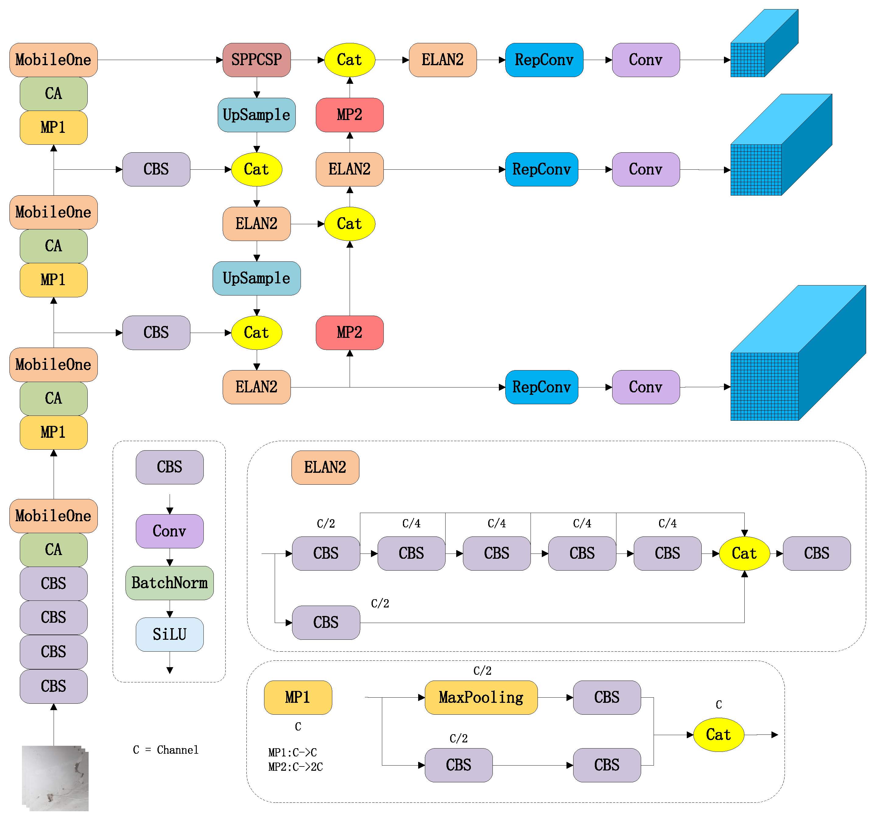
The improved YOLOv7 structure in this paper is shown in Figure 4.

It can be divided into the backbone and the head. The function of the backbone network is to extract features. The original backbone of YOLOv7 is composed of several CBS, MP, and ELAN modules. The CBS is a module consisting of convolution kernel, batch normalization, and SiLU activation function. The MP is consisting of MaxPooling and CBS. The improved backbone replaced the ELAN module with the MobileOne module to increase speed, and a coordinate attention module was added after each MobileOne module. The proposed improvement method has the capability to attend to salient features and suppress extraneous information in the input image, thereby improving detection accuracy effectively.

The head of the network is a PaFPN structure, which consists of a SPPCPC, several ELAN2, CatConv, and three RepVGG blocks. The design of ELAN adopts the gradient path design strategy. In contrast to the data path design strategy, the gradient path design strategy focuses on analyzing the sources and composition of gradients to design network architectures that effectively utilize network parameters. The implementation of this strategy can make the network architecture more lightweight. The distinction between ELAN and ELAN2 lies in the difference in their number of channels. The structural re-parameterization method is applied to the RepVGG block. A multi-branch structure for training and a single-branch structure for inference were used by this method to improve the performance during training and the speed during inference. After outputting three feature maps, the head generates three different-sized prediction results through three RepConv modules.

3.1. MobileOne Module

Calculating cost is an important factor to consider for building façade defects detection. The question of how to enhance computational efficiency while maintaining the efficacy of network detection is of significant value. Generally, there exists a positive correlation between the accuracy of a model and its complexity. However, the increase in complexity will reduce the inference speed of the model and decrease memory utilization [35]. To solve this problem, MobileOne module is incorporated into the YOLOv7’s backbone. MobileOne is an efficient backbone network. In order to maintain the advantages of multi-branch structures during training and the advantages of regular structures during inference, over-parametrization and re-parametrization methods are used to alter the network architecture. Specifically, an over-parametrization structure is used for training and a re-parametrization structure is used for inference to build the network. The reduction in model parameters brought about by re-parameterization can improve the inference performance of the network.

3.1.1. Over-Parametrization Structure

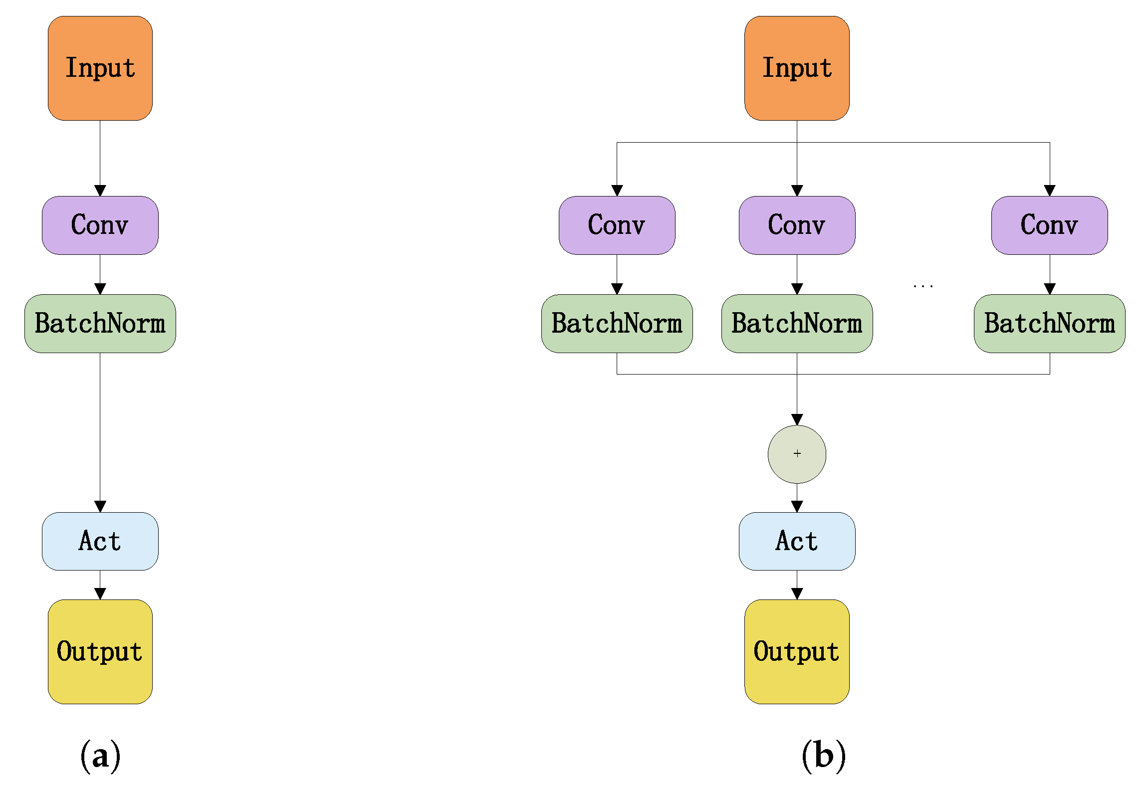
The regular convolution kernel and the over-parameterized convolution kernel are illustrated in Figure 5a and Figure 5b, respectively.

The regular convolution module is composed of convolution kernel, batch normalization, and activation function. In contrast, several identical parallel branches were contained by over-parameterized convolution and the outputs of all branches are summed before entering the activation function. The addition of branching structures can enhance the representational capacity of the model. By increasing the complexity during training, the performance of the model has been improved.

3.1.2. Re-Parametrization Structure

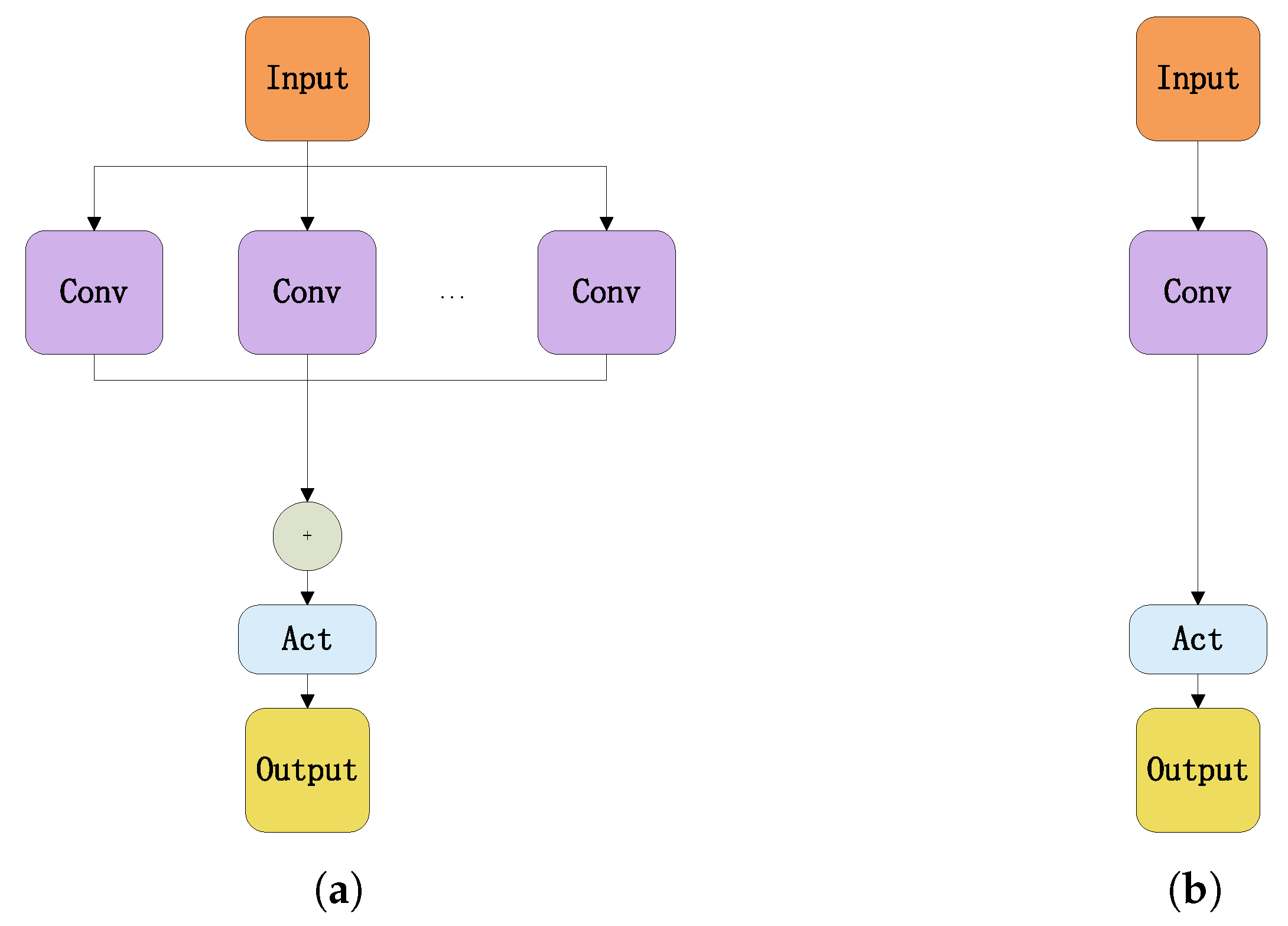
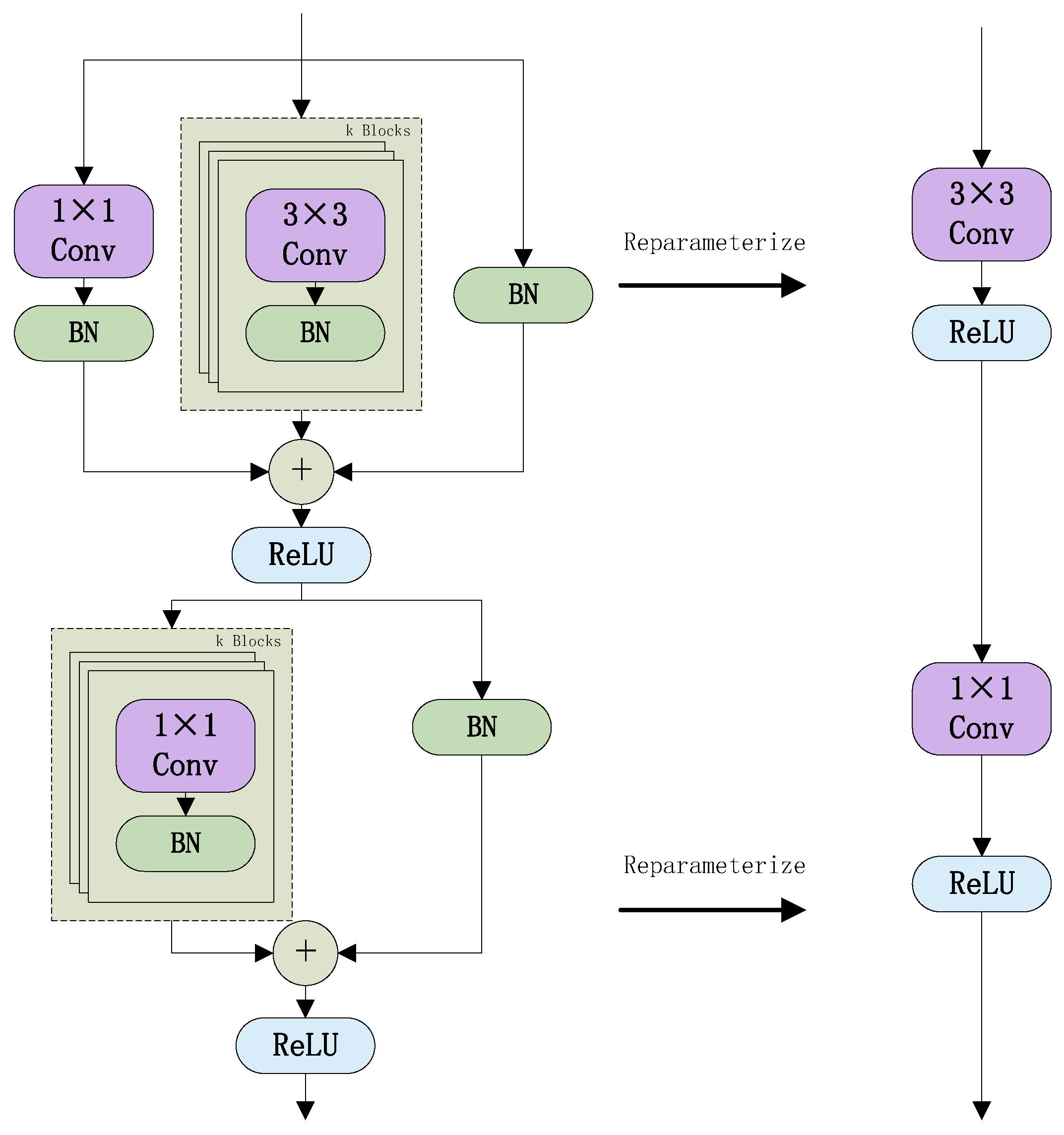
The re-parameterization process is shown in Figure 6. For multiple convolution modules with the same hyperparameters, every Conv-BN branch can be merged into a single convolution module by using the convolution and BN merge method, and all convolution modules can be combined into a new convolution module by using the multi-branch sum method. In the inference phase, the over-parameterized module has only one convolution module and one activation function module, the same as the regular convolution module. The transformation of the multi-branch structure into a single-branch structure results in a reduction in the number of parameters and inference time of the model.

3.1.3. MobileOne Module

The primary structure of MobileOne module is analogous to that of MobileNetV1, with the key distinction being the integration of over-parameterization and re-parameterization methods. MobileOne module structure is shown in Figure 7. The left-hand side of Figure 7 shows the structure of MobileOne module during training, which is composed of a depthwise convolution layer in the upper half and a pointwise convolution layer in the lower half. Depthwise convolution layer is essentially a grouped convolution, which is composed of three branches. The left branch is a $1\times 1$ Conv, the middle branch has k over-parameterized $3\times 3$ convolutions, and the right branch is a jump connection containing a batch normalization. The number of convolutional groups is equivalent to the quantity of input channels. The pointwise convolution layer is composed of two branches, the left branch has k over-parameterized $1\times 1$ convolutions, and the right branch is a jump connection containing a batch normalization. In this paper, k is set at 4.

The right-hand side of Figure 7 shows the structure of MobileOne module during inference. The upper and lower parts are the re-parameterized structure of depthwise convolution layer and pointwise convolution layer, respectively. Depthwise convolution consists of three branches. In the first branch of depthwise convolution, the zero padding method is used to convert the $1\times 1$ convolution kernel to a $3\times 3$ convolution kernel. This $3\times 3$ convolution kernel is merged with the batch normalization to become the first new $3\times 3$ convolution kernel. Equations (1) and (2) are used to calculate the weights ${\omega }^{\prime }$ and biases $b^{\prime }$ of the new convolution kernel.

$${\omega }^{\prime }=\frac{\gamma \ast \omega }{\sqrt{{\sigma }^2+\epsilon }}$$

(1)

$$b^{\prime }=\beta +\gamma \ast \frac{b-\mu }{\sqrt{{\sigma }^2+\epsilon }}$$

(2)

where $\omega$ and b are the weights and biases of the convolution, $\gamma$, $\beta$, $\mu$, and ${\sigma }^2$ are the weights, biases, means, and variances of batch normalization, and $\epsilon$ is a small value to prevent division by zero. The merging of the convolution and batch normalization in the second branch utilizes the same methodology. The parameters of the k convolution kernel are summed after the merger to become the second new $3\times 3$ convolution kernel. The third branch has no convolution layer, so a $3\times 3$ convolution kernel is built before the batch normalization layer to ensure that the three branches can be fused. The $3\times 3$ convolution kernel is merged with the batch normalization to form the third new $3\times 3$ convolution kernel. These three new $3\times 3$ convolution kernels are fused to form the re-parameterized structure of depthwise convolution. The same method is used for the re-parameterized structure of pointwise convolution.

3.2. Coordinate Attention Module

Some defects are challenging to detect by the detector due to the effects of light, weather, background, size, and shape. In order to highlight the features in the image that are beneficial for detection, suppress the noise that causes interference, and make the network focus on a part of the image rather than the whole region during detection, the coordinate attention (CA) module is added to YOLOv7.

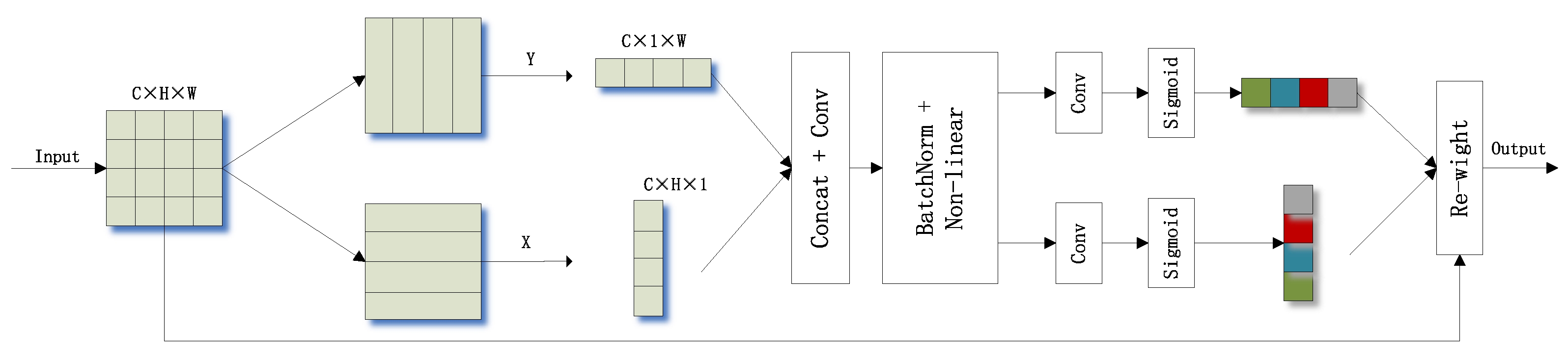
Channel attention mechanisms (e.g., SE, GSoP) [36,37] and spatial attention mechanisms (e.g., EMANet) [38] have achieved significant results. However, channel attention mechanisms only consider inter-channel information and ignore location information, while spatial attention mechanisms can only extract local relations and cannot extract long-distance relations. A lightweight channel attention mechanism called coordinate attention is proposed by Hou, Q et al. to solve these problems. The processing of CA is shown in Figure 8. It can be seen that CA encodes horizontal and vertical location information into channel attention, which allows the network to focus on an extensive range of location information without incurring excessive computational effort.

Coordinate attention encodes channel relationships and long-term dependencies by precise location information, which can be divided into two steps: coordinate information embedding and coordinate attention generation.

3.2.1. Coordinate Information Embedding

The global pooling approach is usually used for global encoding in the channel attention mechanism. However, this approach compresses the global spatial information into the channel descriptors, making it difficult to preserve crucial spatial information. For the input X, CA encodes features from two directions, horizontal and vertical, by using pooling kernels $(H,1)$ and $(1,W)$, respectively, which enables the attention module to capture remote spatial interactions with precise location information. The global pooling approach is decomposed according to the following Equation (3).

$$z_c=\frac{1}{H\times W}\sum _{i=1}^H\sum _{j=1}^W{x}_c\left(i,j\right)$$

(3)

According to Equation (3), the output of the c dimension feature is

$$z_c^h\left(h\right)=\frac{1}{W}\sum _{0\le i<W}{x}_c\left(h,i\right)$$

(4)

$$z_c^w\left(w\right)=\frac{1}{H}\sum _{0\le j<W}{x}_c\left(j,w\right)$$

(5)

These two transformations ((4) and (5)) output two direction-aware feature maps that integrate features from the horizontal and vertical directions, respectively.

3.2.2. Coordinate Attention Generation

The above operation can obtain global receptive field and positional information, and the intermediate feature containing both horizontal and vertical spatial information f can obtained by connecting $z_c^h\left(h\right)$ and $z_c^w\left(w\right)$ with a $1\times 1$ convolution kernel $F_1$ through Equation (6)

$$f=\delta \left(F_1\left(\left[Z^h,Z^w\right]\right)\right),f\in {\mathbb{R}}^{C/r\times \left(H+W\right)}$$

(6)

where $Z^h$ is the output of all channels at the height h, $Z^w$ is the output of all channels at the width w, $\delta$ is the activation function, and r is the ratio of downsampled. Subsequently, f is divided horizontally and vertically into two independent feature maps $f^h$ and $f^w$. Then, convolution and activation are performed on $f^h$ and $f^w$ to obtain the horizontal and vertical attention weights $g^h$ and $g^w$ by Equations (7) and (8)

$$g^h=\sigma \left(F_h\left(f^h\right)\right)$$

(7)

$$g^w=\sigma \left(F_w\left(f^w\right)\right)$$

(8)

where $F_h$ and $F_w$ are $1\times 1$ convolution kernels, and $\sigma$ is the Sigmoid function.

Finally, $g^h$ and $g^w$ are combined into a weight matrix and the $output$ of the coordinate attention mechanism is calculated using Equation (9).

$$output=x_c\left(i,j\right)\times g_c^h\left(i\right)\times g_c^w\left(j\right)$$

(9)

where $g_c^h\left(i\right)$ denotes the horizontal attention weight for height i on channel c, and $g_c^w\left(j\right)$ denotes the vertical attention weight for width j on channel c.

The transitions in coordinate attention are concise and efficient. By utilizing positional information to locate areas of interest while effectively capturing the relationships between channels, the ability to identify targets is enhanced.

3.3. SIoU Loss

In the object detection algorithm, many bounding boxes with high confidence are generated around the real target, and the non-maximum suppression (NMS) algorithm is used to remove the duplicate bounding boxes so that there is only one detection box for each object. The conventional NMS algorithm generates bounding boxes based on object detection scores. Firstly, the list of candidate boxes is sorted in descending order according to the confidence level. Then, the bounding box A with the highest confidence level is selected, added to the output list, and removed from the list of bounding boxes. Finally, the intersection over union (IoU) values of A and all detected boxes in the candidate box list are calculated, and the bounding boxes larger than the threshold value (the threshold value is usually chosen as 0.5) are removed. The algorithm keeps repeating the above process until the list of bounding boxes is empty and returns the output list.

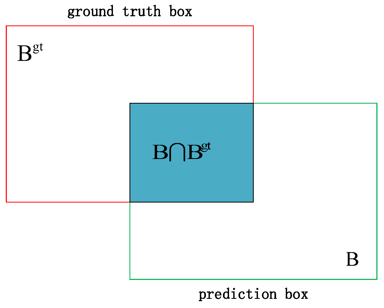
The IoU refers to the ratio of the intersection area and union area of the predicted box and the ground truth box, as shown in Figure 9. Equations (10) and (11) are the equations for IoU and the IoU loss

$$IoU=\frac{\left|B\cap B^{gt}\right|}{\left|B\cup B^{gt}\right|}$$

(10)

$$L_{IoU}=1-\frac{\left|B\cap B^{gt}\right|}{\left|B\cup B^{gt}\right|}$$

(11)

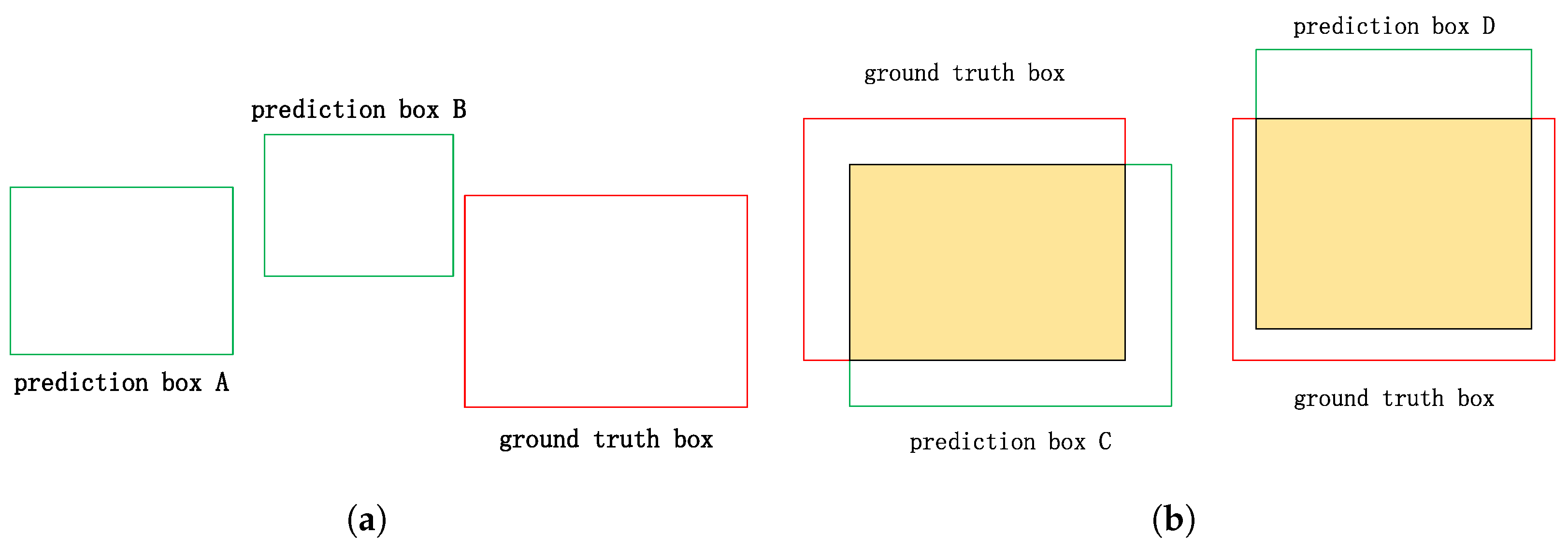
where B is the predicted box and $B^{gt}$ is the ground truth box. The value of $L_{IoU}$ is positively correlated with the degree of overlap between the predicted box and the ground truth box. The IoU is widely applied in object detection algorithms. Nevertheless, there are two issues with IoU, as shown in Figure 10. Figure 10a shows one scenario. Two predicted boxes, A and B, have no intersection with the ground truth box. According to Equation (11), their losses are both 1. However, predicted box B is closer to the ground truth box than predicted box A; therefore, the loss of predicted box B should be smaller. Figure 10b shows the other scenario. Predicted boxes C and D differ in their spatial relationships with the ground truth box. Yet, the loss remains the same for both. It is difficult to determine which predicted box is more accurate in this situation. These existing problems lead to less efficient convergence of IoU.

Compared with the IoU, the SIoU considers not only the overlapping area, distance, and aspect but also the angle between two bounding boxes. The SIoU loss function consists of four cost functions, which are angle cost, distance cost, shape cost, and IoU cost.

3.3.1. Angle Cost

In the early stage of training an object detection network, the situation that the predicted box and the ground truth box do not intersect often happens. Therefore, how to quickly converge the distance between the predicted box and the ground truth is a question worthy of consideration. The SIoU first determines which direction is closer between the predicted box and the ground truth box in X-axis and Y-axis. Then, it moves towards the ground truth box in the closer direction. 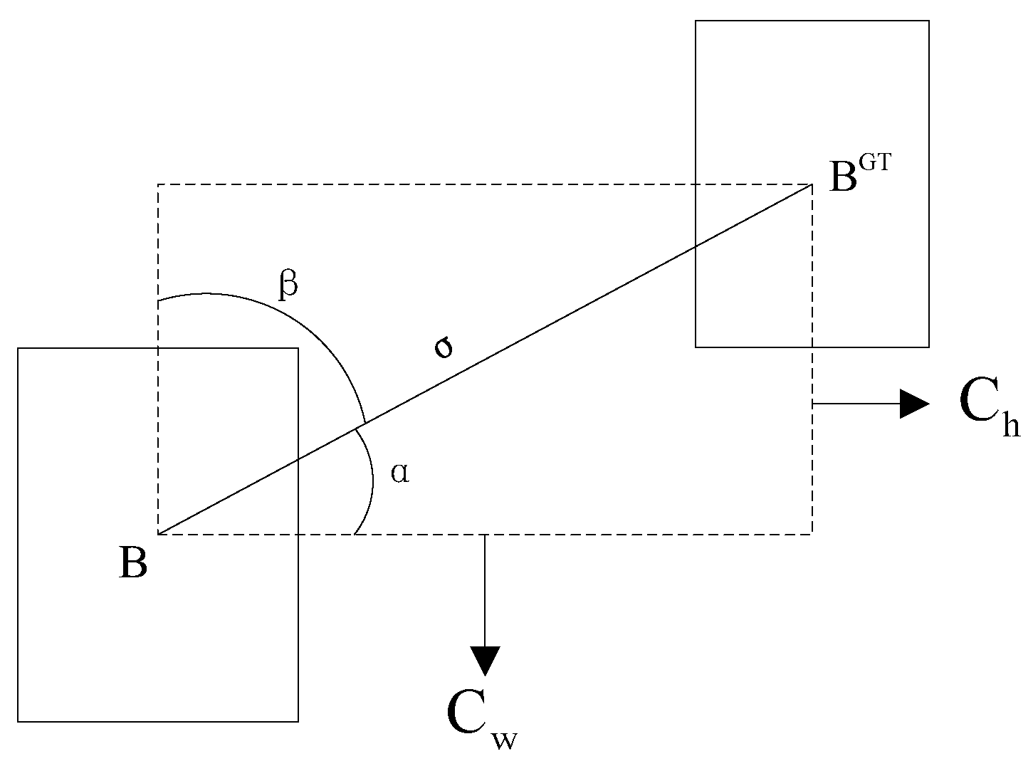Figure 11 shows the boundary regression of SIoU, where $\alpha$ is the angle between the line connecting the center points of the two boxes and the x-axis, $\beta$ is the angle with the y-axis, $C_h$ is the height difference between the center point of the ground truth box and the predicted box, and $\sigma$ is the distance between the center point of the real box and the predicted box.

If $\alpha \le {45}^{\circ }$, the convergence process will first minimize $\alpha$ and otherwise minimize $\beta$. The angle cost $\mathrm{\Lambda }$ is calculated by Equations (12) and (13)

$$\mathrm{\Lambda }=1-2\ast {sin}^2\left(arcsin\left(x\right)-\frac{\pi }{4}\right)$$

(12)

$$x=\frac{C_h}{\sigma }=sin\left(\alpha \right)$$

(13)

3.3.2. Distance Cost

The distance cost $\mathrm{\Delta }$ is calculated by Equations (14) and (15)

$$\mathrm{\Delta }=2-e^{-{\gamma \rho }_x}-e^{-{\gamma \rho }_y}$$

(14)

$${\rho }_x={\left(\frac{b_{c_x}^{gt}-b_{c_x}}{c_w}\right)}^2,{\rho }_y={\left(\frac{b_{c_y}^{gt}-b_{c_y}}{c_h}\right)}^2,\gamma =2-\mathrm{\Lambda }$$

(15)

where ${\rho }_x$ and ${\rho }_y$ represent the distance error in horizontal and vertical directions, respectively. $c_w$ and $c_h$ are the width and height of the smallest external rectangle of the ground truth and predicted boxes, and $\mathrm{\Lambda }$ is the angle cost calculated in the previous section.

3.3.3. Shape Cost

The calculation formula of shape cost $\mathrm{\Omega }$ is as follows.

$$\mathrm{\Omega }=\sum _{t=w,h}{\left(1-e^{-{\omega }_t}\right)}^{\theta }$$

(16)

$${\omega }_w=\frac{\left|w-w^{gt}\right|}{max\left(w,w^{gt}\right)},{\omega }_h=\frac{\left|h-h^{gt}\right|}{max\left(h,h^{gt}\right)}$$

(17)

where ${\omega }_w$ and ${\omega }_h$ represent the normalization coefficients in the horizontal and vertical directions, respectively. $\theta$ indicates the degree of concern about shape cost, which takes values between 2 and 6 depending on the dataset, and $\theta$ is set to 4 in this paper.

3.3.4. IoU Cost

The IoU cost in SIoU is the same as the normal IoU and is calculated using (10). The overall loss calculation formula for SIoU is shown below.

$$L_{SIoU}=1-IoU+\frac{\mathrm{\Delta }+\mathrm{\Omega }}{2}$$

(18)

Compared with the traditional IoU algorithm, SIoU considers the angle between the predicted box and the ground truth box and proposes a more accurate loss calculation method, which is conducive to improving the accuracy and efficiency of the regression. Therefore, SIoU is used by BFD-YOLO as the loss function.

4. Results and Discussion

4.1. Experimental Platform and Parameter Settings

An experimental platform was built for training the model and performing tests. The hardware and software configuration of the experimental platform are shown in

Table 2. Experimental platform.

Equipment	Name
System	Windows 10
CPU	i7-11700
GPU	RTX 3060 12 GB
RAM	32 GB
Programming Languages	Python 3.7
Deep Learning Framework	Pytorch 1.11.0

. In this study, the Stochastic Gradient Descent (SGD) optimizer was employed for model training, with a momentum of 0.937 and a weight decay rate of 0.0005. Lr0 and lrf were set to 00.1 and 0.1, respectively, which means the initial learning rate was 0.01 and the final learning rate was 0.1 times the initial learning rate. Further, five epochs of warm-up training were conducted to make the model fit the data better. The warm-up training method allows the model to stabilize in the first few epochs and then train at the preset learning rate to converge faster. All experiments were performed with 150 epochs, with the batch size set to 16.

4.2. Evaluation Index

The evaluation metrics used in the experiments of this paper are F1 score (F1), precision (P), recall (R), mean average precision ([email protected]), parametric number (Params), and frames per second (FPS). These are common evaluation metrics for object detection [39]. Precision is used to evaluate the error detection rate; recall is used to evaluate the miss detection rate. The F1 score is the harmonic mean of precision and recall, used to evaluate the detection accuracy of the model. Mean average precision is used to evaluate the average accuracy of all categories; the parametric number is used to evaluate the complexity of the model. Frames per second is used to evaluate the detection inference speed of the network, indicating the number of images that the model can process per second. The evaluation metrics are calculated as follows.

$$P=\frac{TP}{TP+FP}$$

(19)

$$R=\frac{TP}{TP+FN}$$

(20)

$$F1=\frac{2\times P\times R}{P+R}$$

(21)

$$AP=\frac{TP+TN}{N}$$

(22)

$$mAP=\frac{1}{n}\sum _{i=1}^n{AP}_i$$

(23)

$$FPS=\frac{1000}{T_f}$$

(24)

where $TP$ denotes the number of positive samples predicted as positive class. $FP$ denotes the number of negative samples predicted as positive class. $FN$ denotes the number of positive samples predicted as negative class. The suffix @.5 in [email protected] indicates that the IoU threshold is taken to be greater than 0.5. n indicates the number of all samples. $T_f$ represents the time required for the model to infer an image, in milliseconds.

4.3. Detection Effect of Different Defects

Representative scenes involving the three defect types were selected as shown in Figure 12. The BFD-YOLO based on MobileOne, CA, and SIoU was used to exhibit the detection effect. The three-colored inspection boxes represent delamination, spalling, and tile loss, respectively. The confidence level of the detection box is indicated by the number above the box, which represents whether the model can effectively detect defects of the façade.

Table 3. Detection results.

Types	Precision (%)	Recall (%)	[email protected] (%)	F1 (%)
Delamination	76.6	70.3	77.8	73.3
Spalling	83.8	79.2	83.8	81.4
Tile loss	84.4	83.9	85.6	84.1
Average	81.6	77.8	82.4	79.7

presents the detection performance for each type of defect and the average detection performance.

It can be observed from Table 3 that the precision, recall, and [email protected] of the three types achieved 81.6%, 77.8%, and 82.4%, respectively. There are some differences in the detection effect of each type of defects. This suggests that the improved network performs relatively better in recognizing spalling and tile loss, but its performance in delamination is comparatively lower. Overall, the model demonstrates satisfactory performance and meets the precision requirements for façade detection.

4.4. Ablation Experiments

Five sets of ablation experiments, including YOLOv7, coordinate attention-based YOLOv7 (CA-YOLOv7), SIoU-based YOLOv7 (SIoU-YOLOv7), MobileOne-based YOLOv7 (MobileOne-YOLOv7), and our proposed method for building façade defects detection (BFD-YOLO), were performed to verify the effectiveness of the improvements proposed in this paper. The recall and [email protected] curves of models employing different improvements are depicted in Figure 13. It can be seen from Figure 13 that the MobileOne module effectively enhances the accuracy of the model, while the CA and SIoU modules improve the recall.

The combination of the three improvements results in significant improvements of BFD-YOLO over the original YOLOv7 in terms of both accuracy and recall. The results of the ablation experiments are shown in

Table 4. Ablation experiment results.

Model Name	Precision (%)	Recall (%)	[email protected] (%)	F1 (%)	Params	FPS
YOLOv7	79.4	75.7	79.5	77.5	36,492,560	83
MobileOne-YOLOv7	77.6	74.2	77.4	75.9	32,602,512	101
CA-YOLOv7	81.2	77.1	82.2	79.1	36,719,104	59
SIoU-YOLOv7	79.3	77.0	81.5	78.1	36,492,560	81
MobileOne-CA-YOLOv7	80.7	76.4	81.8	78.5	34,140,800	77
BFD-YOLOv7	81.6	77.8	82.4	79.7	34,140,800	76

.

The first set of experiments uses original YOLOv7 as the benchmark. The MobileOne module was integrated in YOLOv7 in the second set of experiments. Its precision and [email protected] decreased 1.8% and 2.1%, respectively. Nevertheless, there was a reduction of 10.6% in the number of parameters, while the FPS achieved 101. The CA module was incorporated into YOLOv7 in the third set of experiments. There was an increase in the number of model parameters and inference speed, but precision was improved by 1.8% and [email protected] was improved by 2.7%. SIoU was used to replace the original IoU in the fourth set of experiments; the recall and accuracy of the model increased by 1.3% and 2%, respectively. The fifth set of experiments combined the MobileOne module and the CA module. Compared with the second group of experiments, the addition of the CA module has enhanced the ability of the network to acquire features, and both the accuracy and recall have been improved. However, the extra computation brought by the CA module also reduces the inference speed of the model by 23.8%. The sixth set of experiments combined three improvement methods. It achieved an accuracy of 81.6%, recall of 77.8%, and [email protected] of 82.4%, exhibiting the optimal detection performance.

4.5. Comparative Analysis of Different Models

Ablation experiments demonstrate the effectiveness of the proposed improvements in this paper, while further comparative evaluations are required to determine whether our method has reached a competitive performance level. Experiments were conducted on YOLOv5 [40], RetinaNet [41], and Faster R-CNN [21] using the dataset proposed in this paper and were compared with the BFD-YOLO. The official default configuration was used for the training of YOLOv5, RetinaNet, and Faster R-CNN. Specifically, the YOLOv5l model was selected, momentum was set to 0.937, weight decay rate was set to 0.0005, and the number of warm-up epochs was set to three during training of YOLOv5. Resnet50 was chosen as the backbone network, momentum was set to 0.9, and weight decay rate was set to 0.0005 by both RetinaNet and Faster R-CNN. SGD was adopted for the training of the three models. Different models’ training results are shown in Figure 14. It can be observed from Figure 14 that our method achieves higher recall and [email protected] than the other methods.

Figure 15 shows the training loss function curves of the five methods. The class loss is used to determine the consistency between anchor boxes label and their true label, while box loss is used to measure the error between predicted boxes and ground truth boxes. It can be observed that our proposed method effectively enhances the correctness of the classification process and the precision of the anchor box process.

Table 5. Comparative experiment results.

Methods	Precision (%)	Recall (%)	[email protected] (%)	F1 (%)	FPS
BFD-YOLO	81.6	77.8	82.4	79.7	76
YOLOv5l	76.2	73.4	77.9	74.8	64
RetinaNet	73.1	70.5	73.8	71.8	35
Faster R-CNN	75.4	73.7	77.2	74.5	17

shows the comparative experiment results of four models. It can be observed that YOLOv5l slightly outperforms Faster R-CNN in accuracy and has an advantage in speed. The performance of RetinaNet is not satisfactory, and BFD-YOLO demonstrates the best performance in terms of accuracy and efficiency among the four models.

In order to verify the generalization ability of the model proposed in this paper, we selected images from the test set that contained small targets and complex backgrounds for comparison, and the detection results are shown in Figure 16, Figure 17 and Figure 18.

The results show that other methods have phenomena of missed detection and false detection in complex environments and when detecting small targets, while BFD-YOLO maintains an accurate detection. These results indicate that the improved method proposed in this paper effectively enhances the performance of exterior façade defect detection.

5. Conclusions

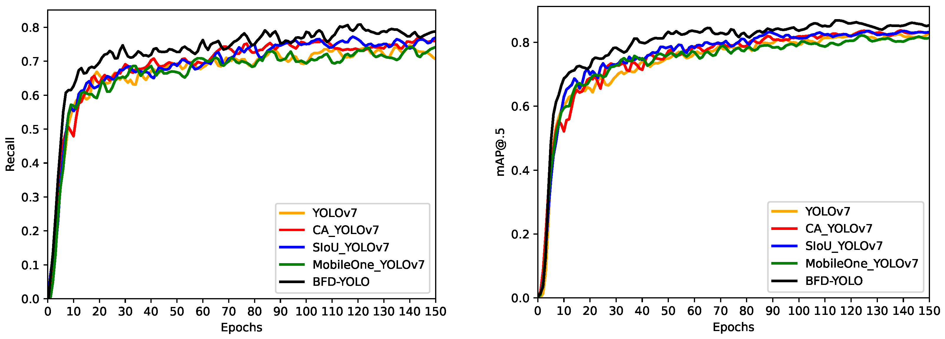
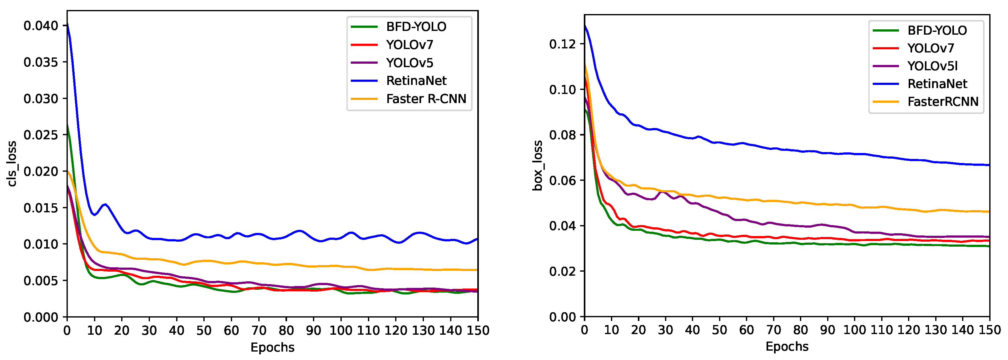
This paper proposes an improved YOLOv7 façade defects detection method named BFD-YOLO, which can achieve high speed and accurate detection of façade defects on buildings. The experimental analysis shows that the incorporation of over-parametrization and re-parameterization methods enables the model to efficiently acquire more features, and the incorporation of the MobileOne module can reduce the parameter amount and complexity of the network, thus decreasing the inference time effectively. The coordinate attention takes into account inter-channel information and orientation-related positional information, which helps the model to better localize and identify targets. So, the combination of coordinate attention and YOLOv7 can effectively enhance the feature extraction capability and improve the object detection accuracy of the network. SIoU added the orientation factor to the calculation of IoU and redefined the penalty metrics to more accurately reflect the relationship between the predicted box and the ground truth box and improve the convergence speed of the model. The utilization of SIoU effectively improves the recall rate and enhances the convergence ability of the network. Based on the original YOLOv7, the precision of BFD-YOLO increased by 2.2%, while its recall and [email protected] increased by 2.1% and 2.9%, respectively. In comparison to other models, this method has obvious advantages and the FPS of 76 can meet the requirements of real-time detection. Moreover, we expanded on the open dataset to construct a dataset containing three types of façade defects.

Currently, the development trend of building façade defect detection is automation and intelligence. The method proposed in this paper can help realize this goal. We are now trying to use the industrial-grade drone (Phantom 4 RTK) to automatically photograph building façades on a planned flight path and detect defects using BFD-YOLO on real-time image transfer data. The detected damage will be localized to the 3D reconstruction model of the building. In future research, we will expand the type and number of the dataset to increase the types of defects that can be detected by the proposed method. Meanwhile, we will explore more effective methods to improve the accuracy and speed of defect detection.

References

1. Lee, J.S. Value engineering for defect prevention on building façade. J. Constr. Eng. Manag. 2018, 144, 04018069. [Google Scholar] [CrossRef]
2. Chong, W.K.; Low, S.P. Latent building defects: Causes and design strategies to prevent them. J. Perform. Constr. Facil. 2006, 20, 213–221. [Google Scholar] [CrossRef]
3. Faqih, F.; Zayed, T.; Soliman, E. Factors and defects analysis of physical and environmental condition of buildings. J. Build. Pathol. Rehabil. 2020, 5, 19. [Google Scholar] [CrossRef]
4. ASTM F2659; Standard Guide for Preliminary Evaluation of Comparative Moisture Condition of Concrete, Gypsum Cement and Other Floor Slabs and Screeds Using a Non-Destructive Electronic Moisture Meter. ASTM: West Conshohocken, PA, USA, 2015.
5. Guo, J.; Wang, Q.; Li, Y. Semi-supervised learning based on convolutional neural network and uncertainty filter for façade defects classification. Comput.-Aided Civ. Infrastruct. Eng. 2021, 36, 302–317. [Google Scholar] [CrossRef]
6. Ye, X.; Jin, T.; Yun, C. A review on deep learning-based structural health monitoring of civil infrastructures. Smart Struct. Syst. 2019, 24, 567–585. [Google Scholar]
7. Kim, S.; Frangopol, D.M.; Zhu, B. Probabilistic optimum inspection/repair planning to extend lifetime of deteriorating structures. J. Perform. Constr. Facil. 2011, 25, 534–544. [Google Scholar] [CrossRef]
8. Anuar, M.Z.T.; Sarbini, N.N.; Ibrahim, I.S.; Osman, M.H.; Ismail, M.; Khun, M.C. A comparative of building condition assessment method used in Asia countries: A review. IOP Conf. Ser. Mater. Sci. Eng. 2019, 513, 012029. [Google Scholar] [CrossRef]
9. Vilhena, A.; Costa Branco De Oliveira Pedro, J. Portuguese method for buildings’ Condition assessment: Analysis of the first three years of application. In Proceedings of the Building a Better World: CIB World Congress, Salford, UK, 10–13 May 2010. Citeseer. [Google Scholar]
10. D’Aloisio, J.A. Structural building condition reviews: Beyond distress. In Proceedings of the Structures Congress, Denver, CO, USA, 6–8 April 2017; pp. 289–301. [Google Scholar]
11. Faqih, F.; Zayed, T. Defect-based building condition assessment. Build. Environ. 2021, 191, 107575. [Google Scholar] [CrossRef]
12. Shariq, M.H.; Hughes, B.R. Revolutionising building inspection techniques to meet large-scale energy demands: A review of the state-of-the-art. Renew. Sustain. Energy Rev. 2020, 130, 109979. [Google Scholar] [CrossRef]
13. Riveiro, B.; Solla, M. Non-Destructive Techniques for the Evaluation of Structures and Infrastructure; CRC Press: Boca Raton, FL, USA, 2016; Volume 11. [Google Scholar]
14. Zhao, Y.; Li, T.; Zhang, X.; Zhang, C. Artificial intelligence-based fault detection and diagnosis methods for building energy systems: Advantages, challenges and the future. Renew. Sustain. Energy Rev. 2019, 109, 85–101. [Google Scholar] [CrossRef]
15. Ghosh Mondal, T.; Jahanshahi, M.R.; Wu, R.T.; Wu, Z.Y. Deep learning-based multi-class damage detection for autonomous post-disaster reconnaissance. Struct. Control. Health Monit. 2020, 27, e2507. [Google Scholar] [CrossRef]
16. Perez, H.; Tah, J.H. Deep learning smartphone application for real-time detection of defects in buildings. Struct. Control. Health Monit. 2021, 28, e2751. [Google Scholar] [CrossRef]
17. Girshick, R.; Donahue, J.; Darrell, T.; Malik, J. Rich feature hierarchies for accurate object detection and semantic segmentation. In Proceedings of the IEEE Conference on Computer Vision and Pattern Recognition, Columbus, OH, USA, 23–28 June 2014; pp. 580–587. [Google Scholar]
18. Redmon, J.; Divvala, S.; Girshick, R.; Farhadi, A. You only look once: Unified, real-time object detection. In Proceedings of the IEEE Conference on Computer Vision and Pattern Recognition, Las Vegas, NV, USA, 27–30 June 2016; pp. 779–788. [Google Scholar]
19. Liu, W.; Anguelov, D.; Erhan, D.; Szegedy, C.; Reed, S.; Fu, C.Y.; Berg, A.C. Ssd: Single shot multibox detector. In Proceedings of the European Conference on Computer Vision, Amsterdam, The Netherlands, 11–14 October 2016; Springer: Cham, Switzerland, 2016; pp. 21–37. [Google Scholar]
20. Uijlings, J.R.; Van De Sande, K.E.; Gevers, T.; Smeulders, A.W. Selective search for object recognition. Int. J. Comput. Vis. 2013, 104, 154–171. [Google Scholar] [CrossRef]
21. Ren, S.; He, K.; Girshick, R.; Sun, J. Faster r-cnn: Towards real-time object detection with region proposal networks. Adv. Neural Inf. Process. Syst. 2015, 28, 91–99. [Google Scholar] [CrossRef]
22. Girshick, R. Fast r-cnn. In Proceedings of the IEEE International Conference on Computer Vision, Santiago, Chile, 7–13 December 2015; pp. 1440–1448. [Google Scholar]
23. Samhouri, M.; Al-Arabiat, L.; Al-Atrash, F. Prediction and measurement of damage to architectural heritages facades using convolutional neural networks. Neural Comput. Appl. 2022, 34, 18125–18141. [Google Scholar] [CrossRef]
24. Lee, K.; Hong, G.; Sael, L.; Lee, S.; Kim, H.Y. MultiDefectNet: Multi-class defect detection of building façade based on deep convolutional neural network. Sustainability 2020, 12, 9785. [Google Scholar] [CrossRef]
25. Guo, J.; Wang, Q.; Li, Y. Evaluation-oriented façade defects detection using rule-based deep learning method. Autom. Constr. 2021, 131, 103910. [Google Scholar] [CrossRef]
26. Mishra, M.; Barman, T.; Ramana, G. Artificial intelligence-based visual inspection system for structural health monitoring of cultural heritage. J. Civ. Struct. Health Monit. 2022, 1–18. [Google Scholar] [CrossRef]
27. Idjaton, K.; Desquesnes, X.; Treuillet, S.; Brunetaud, X. Transformers with yolo network for damage detection in limestone wall images. In Proceedings of the International Conference on Image Analysis and Processing, Lecce, Italy, 23–27 May 2022; Springer: Cham, Switzerland, 2022; pp. 302–313. [Google Scholar]
28. Liu, C.; Sui, H.; Wang, J.; Ni, Z.; Ge, L. Real-Time Ground-Level Building Damage Detection Based on Lightweight and Accurate YOLOv5 Using Terrestrial Images. Remote Sens. 2022, 14, 2763. [Google Scholar] [CrossRef]
29. Wang, C.Y.; Bochkovskiy, A.; Liao, H.Y.M. YOLOv7: Trainable bag-of-freebies sets new state-of-the-art for real-time object detectors. arXiv 2022, arXiv:2207.02696. [Google Scholar]
30. Lin, T.Y.; Maire, M.; Belongie, S.; Hays, J.; Perona, P.; Ramanan, D.; Dollár, P.; Zitnick, C.L. Microsoft coco: Common objects in context. In Proceedings of the European Conference on Computer Vision, Zurich, Switzerland, 6–12 September 2014; Springer: Cham, Switzerland, 2014; pp. 740–755. [Google Scholar]
31. Vasu, P.K.A.; Gabriel, J.; Zhu, J.; Tuzel, O.; Ranjan, A. MobileOne: An Improved One Millisecond Mobile Backbone. In Proceedings of the IEEE/CVF Conference on Computer Vision and Pattern Recognition, Vancouver, BC, Canada, 17–24 June 2023; pp. 7907–7917. [Google Scholar]
32. Hou, Q.; Zhou, D.; Feng, J. Coordinate attention for efficient mobile network design. In Proceedings of the IEEE/CVF Conference on Computer Vision and Pattern Recognition, Nashville, TN, USA, 19–25 June 2021; pp. 13713–13722. [Google Scholar]
33. Gevorgyan, Z. SIoU Loss: More Powerful Learning for Bounding Box Regression. arXiv 2022, arXiv:2205.12740. [Google Scholar]
34. Kung, R.Y.; Pan, N.H.; Wang, C.C.; Lee, P.C. Application of deep learning and unmanned aerial vehicle on building maintenance. Adv. Civ. Eng. 2021, 2021, 5598690. [Google Scholar] [CrossRef]
35. Ding, X.; Zhang, X.; Ma, N.; Han, J.; Ding, G.; Sun, J. Repvgg: Making vgg-style convnets great again. In Proceedings of the IEEE/CVF Conference on Computer Vision and Pattern Recognition, Nashville, TN, USA, 19–25 June 2021; pp. 13733–13742. [Google Scholar]
36. Hu, J.; Shen, L.; Sun, G. Squeeze-and-excitation networks. In Proceedings of the IEEE Conference on Computer Vision and Pattern Recognition, Salt Lake City, UT, USA, 18–23 June 2018; pp. 7132–7141. [Google Scholar]
37. Wang, Q.; Wu, B.; Zhu, P.; Li, P.; Zuo, W.; Hu, Q. ECA-Net: Efficient channel attention for deep convolutional neural networks. In Proceedings of the IEEE/CVF Conference on Computer Vision and Pattern Recognition, Seattle, WA, USA, 13–19 June 2020; pp. 11534–11542. [Google Scholar]
38. Li, X.; Zhong, Z.; Wu, J.; Yang, Y.; Lin, Z.; Liu, H. Expectation-maximization attention networks for semantic segmentation. In Proceedings of the IEEE/CVF International Conference on Computer Vision, Seoul, Republic of Korea, 27 October–2 November 2019; pp. 9167–9176. [Google Scholar]
39. Wan, F.; Sun, C.; He, H.; Lei, G.; Xu, L.; Xiao, T. YOLO-LRDD: A lightweight method for road damage detection based on improved YOLOv5s. EURASIP J. Adv. Signal Process. 2022, 2022, 98. [Google Scholar] [CrossRef]
40. Ultralytics. YOLOv5: A State-of-the-Art Real-Time Object Detection System. 2021. Available online: https://docs.ultralytics.com (accessed on 10 August 2023).
41. Lin, T.Y.; Goyal, P.; Girshick, R.; He, K.; Dollár, P. Focal loss for dense object detection. In Proceedings of the IEEE International Conference on Computer Vision, Venice, Italy, 22–29 October 2017; pp. 2980–2988. [Google Scholar]
Figure 1. Examples of images in dataset. (a) Delamination. (b) Spalling. (c) Tile loss.
Electronics 12 03612 g001
Figure 2. Data augmentation effects. (a) Original image. (b) Rotation. (c) Scaling. (d) Brightness adjustment.
Electronics 12 03612 g002
Figure 3. Instances information. (a) Number of instances. (b) Location of objects. (c) Size of objects.
Electronics 12 03612 g003
Figure 4. Structure of BFD-YOLO.
Electronics 12 03612 g004
Figure 5. Structures of regular and over-parametrization convolution. (a) Regular convolution. (b) Over-parametrization convolution.
Electronics 12 03612 g005
Figure 6. Re-parameterization process. (a) Merger of Conv and BN. (b) Merger of MultiConv branch.
Electronics 12 03612 g006
Figure 7. MobileOne module structure.
Electronics 12 03612 g007
Figure 8. Process of coordinate attention.
Electronics 12 03612 g008
Figure 9. Figure of IoU calculation.
Electronics 12 03612 g009
Figure 10. Two issues of IoU. (a) Scenario 1. (b) Scenario 2.
Electronics 12 03612 g010
Figure 11. Angle cost schematic of SIoU.
Electronics 12 03612 g011
Figure 12. Different defects recognition.
Electronics 12 03612 g012
Figure 13. Comparison of different improvements.
Electronics 12 03612 g013
Figure 14. Comparison of different modules.
Electronics 12 03612 g014
Figure 15. Loss of different modules.
Electronics 12 03612 g015
Figure 16. Detection results of common situations. (a) Original Image. (b) BFD-YOLO. (c) YOLOv5l. (d) RetinaNet. (e) Faster R-CNN.
Electronics 12 03612 g016
Figure 17. Detection results of small objects. (a) Original Image. (b) BFD-YOLO. (c) YOLOv5l. (d) RetinaNet. (e) Faster R-CNN.
Electronics 12 03612 g017
Figure 18. Detection results of complex background. (a) Original Image. (b) BFD-YOLO. (c) YOLOv5l. (d) RetinaNet. (e) Faster R-CNN.
Electronics 12 03612 g018