Article

Application of Vibration Data Mining and Deep Neural Networks in Bridge Damage Identification

1
School of Mechanical Engineering, Guizhou University, Guiyang 550025, China
2
State Key Laboratory of Public Big Data, Guizhou University, Guiyang 550025, China
*
Author to whom correspondence should be addressed.
Electronics 2023, 12(17), 3613; https://doi.org/10.3390/electronics12173613
Submission received: 6 August 2023 / Revised: 20 August 2023 / Accepted: 24 August 2023 / Published: 26 August 2023

Abstract

:
The aim of this paper is to mine the information contained in the bridge health monitoring data as well as to improve the shortcomings of traditional identification methods. In this paper, a bridge damage identification method based on the combination of data mining and deep neural networks is introduced. Firstly, a noise reduction method based on parameter optimisation of wavelet threshold decomposition is proposed, which further removes the noise signal by introducing two adjustment parameters in the threshold function to adapt to different wavelet decomposition layers. Furthermore, the Fast Fourier Transform is used to analyse the feature pattern of the original signal in the frequency domain, and the modal frequency features that exhibit the difference in damage categories are extracted from the spectrogram through sliding windows. Finally, a large number of irrelevant variables with small weight contributions are discarded by principal component analysis, and only the sensitive features with the most informative categories are retained as the input to the deep neural networks. The experimental results show that the new metrics after the feature engineering process improve the ability of damage identification and have stronger robustness, while our damage identification scheme achieves a good balance between the model computation and recognition accuracy. Furthermore, the recognition accuracy of the deep neural networks reaches over 93% with only three feature dimensions retained.

1. Introduction

As one of the transportation facilities in everyday life, bridges make an important contribution to the economic development of a region. Existing bridge structures are vulnerable to damage from factors such as material degradation and external loads during operation. Visual inspection is highly subjective when assessing bridge structures [1], so more and more bridges are being fitted with structural health monitoring systems [2]. These monitoring systems continuously collect various types of sensing data from the bridge, including a dynamic response, a static response, and an apparent morphology, which contain a large amount of damage information and form the basis for assessing the condition of the bridge [3]. Therefore, the interpretation of these data from the perspective of structural safety has become the focus of bridge damage identification research.
To improve the efficiency of damage identification, feature engineering is required to design more sensitive features before algorithmic identification. Features commonly used in data analysis include statistical features, frequency domain features, and time-frequency domain features. Among these, statistical features are usually calculated from existing features to account for their internal uncertainties. Zhang et al. [4] used the mean and standard deviation of data for the reliability analysis of structures. Mattson and Pandit [5] used variance, skewness, and peak values as damage features for structural damage identification.
Frequency domain features, including frequency, mode, and modal strain, have gained wide application over the past few decades [6]. Moughty and Casas [7] used vibration features for analysis in damage detection and system identification. However, this method is insensitive to local and small damages and cannot obtain the complete modal information of the structure. Time-frequency domain features can describe the local details of measurements in both the time and frequency domains and are therefore able to detect changes caused by damage promptly. Some researchers have used wavelet packet component energy [8] and instantaneous frequency after the Hilbert-Huang transform [9] to construct different damage features. Shahsavari et al. [10] and Suarez et al. [11] chose the coefficients and energy ratio of the wavelet transform for damage identification of structures with good results, respectively.
Existing damage identification methods can be divided into model-based and data-driven methods. Model-based approaches predict the outcome by building many mechanical and mathematical computational models [12]. However, the presence of a large amount of monitoring data makes it difficult to build finite element models to reflect information on the properties of the bridge structure, resulting in too little physical interpretability [13]. Data-driven methods can directly analyse measured structural change data, such as probability density functions [14], without any a priori knowledge and can therefore take into account the uncertainties in the raw data.
In recent years, deep learning architectures have shown great promise for automated structural health monitoring processes [15]. Deep learning can be used to obtain higher-level representations by combining lower-level representations. These high-level features can amplify the fundamental parts of the input used for differentiation and suppress irrelevant parts, so their performance will improve with the use of more data, where traditional methods may encounter bottlenecks [16,17].
Bao et al. [18] chose to convert raw time series measurements into image vectors and then input the image vectors into a deep neural network to identify various anomalies. In 2019, Zhenqing Liu et al. [19] used U-Net for the first time to detect concrete cracks, and the trained U-Net was able to accurately identify the crack locations from the original images under different conditions with high robustness. Parisi et al. [20] used finite element models of steel frame bridges under different damage scenarios to obtain strain data, extracted and selected features from the data that were more sensitive to damage, and fed these features into a one-dimensional convolutional neural network (CNN) with an accuracy of 93% for damage identification. In classification applications, recurrent neural networks are used specifically to process sequential data by combining previous outputs and current inputs into the current prediction and are typically used in structural damage recognition for feature extraction and end-to-end classification. For example, long short-term memory (LSTM) is used to classify and diagnose clinical monitoring data with poor data conditions [21]. A deep auto-encoder (DAE) consists of a stack of multiple auto-encoders, which is a three-layer network typically used for dimensionality reduction or feature extraction. Pathirage et al. [22] constructed two variants of a DAE with different hidden layers for early damage detection in bridges, localising and quantifying damage in both numerical and experimental frame structures, showing better performance than the artificial neural network.
For the classification problem of damaged data, most studies choose to take the raw data as input directly or select statistical features such as extreme value, mean, and variance for analysis, but these features can hardly reflect the correspondence between the implicit information of the data and the structural damage. Based on this, the research in this paper consists of the following three parts: the first part is the parameter optimisation of wavelet threshold decomposition; the second part is the feature extraction and selection of structural damage information; and the third part is the damage identification by deep neural networks. Specifically, firstly, the optimisation algorithm of random search introduces two adjustment parameters in the threshold function to accommodate different wavelet decomposition layers. Secondly, in the feature extraction process, the Fast Fourier Transform and sliding window are used to extract modal frequency features in the spectrum that contain differences in damage categories, and then the principal component analysis is used to discard the principal components with small weight contributions and only retain the sensitive features with the largest amount of category information. Finally, different deep neural networks are used for impairment identification, and the corresponding experimental comparisons and performance analyses are conducted.
The remainder of the paper is organised as follows: In Section 2, a brief overview of data processing and neural network-related methods is given. In Section 3, noise reduction methods based on wavelet threshold decomposition with parameter optimisation and feature engineering of the data are described in detail. In Section 4, experiments on damage identification are arranged, and the results are analysed and compared. In Section 5, the full paper is summarised.

2. Research Methods

This paper investigates data pre-processing, feature engineering, and damage identification techniques in the field of bridge monitoring while providing an in-depth analysis of feature dimensions and damage category information and proposing a damage identification method based on a combination of data mining and deep neural networks.

2.1. Wavelet Threshold Decomposition

The wavelet transform is an adaptive time-frequency domain analysis method, and the wavelet transform can be used to decompose different frequency components of the signal, which is very effective for signal decomposition and reconstruction [23].
Assume that the signal is defined by f ( t ) and f ( t ) L 2 ( R ) , whose continuous wavelet transform is defined as follows:
W f a , b = 1 a + f t ψ ^ t b a d t = < f t , ψ a , b t > ,
ψ a , b t = 1 a ψ t b a ,
in which ψ ( t ) is the mother wavelet function, ψ ^ ( ω ) is the Fourier spectrum of ψ ( t ) , and ψ a , b ( t ) is the wavelet basis function after a stretching translational transform, where a and b denote the stretch factor and translation factor, respectively. Another discrete wavelet transform is defined as follows:
W f m , n = a m / 2 + f t ψ a m t n d t .
Wavelet threshold decomposition in the wavelet transform is a simple and effective noise reduction method. By processing the coefficients of each layer with modes greater or less than a set threshold separately, the noise is suppressed to recover the original signal [24]. Figure 1 illustrates the basic principle of wavelet threshold decomposition.
In the above noise reduction process, the selection and design of different parameters can have a significant impact on the signal noise reduction effect. Common evaluation metrics are the signal-to-noise ratio (SNR) and the mean square error (MSE) [25], both of which are calculated as follows:
S N R = 10 log 10 n = 1 N f 2 n n = 1 N f n f n ¯ 2 ,
M S E = 1 N n = 1 N f n f n ¯ 2 .
In Equations (4) and (5), f ( n ) is the original noise-free signal, f ( n ) ¯ is the signal processed by wavelet threshold decomposition after adding noise to f ( n ) , and N denotes the signal length.

2.2. Fast Fourier Transform

The Fourier transform is a fundamental signal processing theory that shows that any continuously measured time-series signal can be represented as an infinite superposition of sinusoids of different frequencies, so that the spectrum of these sinusoids can be analysed to effectively extract the spectral features of the signal that are not visible in the original time domain. The Fast Fourier Transform is based on the properties of the Discrete Fourier Transform, which reduces the computational complexity from N 2 to N × log 10 N , greatly simplifying the computational process. The expression for the Discrete Fourier Transform is as follows:
X k = n = 0 N 1 x n e 2 j π k n / N ,
in which x n is the time domain signal, N denotes the number of samples, k denotes the subscripts of the samples in the frequency domain signal, and X k is the sequence of the obtained frequency domain signals.

2.3. Principal Component Analysis

In the process of data processing, it is often necessary to reduce the dimensionality of feature information in high-dimensional data, with the aim of spatially compressing the high-dimensional data to extract more effective key information. In the actual calculation, the principal component analysis (PCA) constructs the principal components by calculating the eigenvalues and eigenvectors of the correlation matrix between attributes, and the contribution of the principal components is determined based on the magnitude of the eigenvalues [26], discarding the principal components with small weights, which can effectively avoid the problem of overfitting. The calculation process is as follows:
Assuming a dataset of m samples with n features, the matrix X is obtained by decentralising all samples, and the covariance moment is calculated:
C = 1 m 1 × X T X .
The eigenvalues λ k and the corresponding eigenvectors υ k are obtained by eigendecomposition:
C υ k = λ k υ k ,
the eigenvectors are arranged into matrices in order of their corresponding eigenvalue magnitudes, and the first k columns are taken to form a matrix W . The sample features after compression to k dimensions are obtained by Y = X W , a matrix of order m × k .

2.4. Deep Neural Network

With the continuous development of neural networks, deep neural networks have not only achieved great success in imaging but have also started to be used in structured data processing. In this paper, three types of deep neural networks, namely CNN, LSTM, and DAE, are used for damage identification of bridge structure monitoring data. In the structure of a CNN, the first few layers are usually alternating between convolutional and pooling layers, while the last layers near the output consist of fully connected layers responsible for mapping the features extracted by the former to the corresponding damage classes [27]. The structure of a CNN is shown in Figure 2.
LSTM is a variant of a recurrent neural network that offers advantages in its ability to model temporal correlation and accept data of different lengths. By bringing cell states and gating mechanisms into the network, decisions are made as to which information should be saved or discarded while overcoming the effects of short-term memory. DAE is constructed by stacking multiple auto-encoders to learn mapping relationships through a neural network so that the input information can be reconstructed [2]. The advantage is the ability to extract the implicit information behind the data in an unsupervised manner, providing better generalisation capabilities and prediction accuracy. The auto-encoder mainly consists of two parts: the encoder and the decoder. The role of the encoder is to encode the high-dimensional input X into a low-dimensional hidden variable, and the role of the decoder is to restore the hidden variable h in the hidden layer to its initial dimension, X R X .

3. Data Preparation

In this section, the dataset used in this study is first introduced, followed by a detailed description of the noise reduction method based on wavelet threshold decomposition with parameter optimisation, after which feature engineering is proposed to extract and select feature information for the data categories.

3.1. Dataset

The dataset used in this study is derived from the public dataset for structural health monitoring provided by the European Workshop, which is available at http://users.metropolia.fi/~kullj/ (accessed on 12 March 2023), and a detailed description of the dataset is provided in reference [28]. The data is derived from a sequence of y-direction accelerations measured by 47 sensors, each with a certain deviation of Gaussian noise added to reflect the interference from the external environment of the bridge, with an average noise level of approximately 10% of the signal for each measurement of 2859 samples, a data size of 2859 × 47 , and a sampling frequency of 571 Hz. The first 50 measurements are taken from undamaged structures, and the last 50 measurements are taken for five types of damage: Damage 1, Damage 2, Damage 3, Damage 4, and Damage 5, with data measured from different damaged structures.

3.2. Data Pre-Processing

Considering the balance of the dataset, each type of data is randomly down-sampled according to the time series, with 6000 data samples for each type of data and a total of 36,000 data samples for one type of normal sample and five types of damage samples, thus forming the original dataset. Figure 3 illustrates the data distribution.
To eliminate the variability between different dimensions of the data, the original dataset is zero-mean normalised. As the bridge acceleration signal is time series data containing Gaussian noise, this paper proposes to use a wavelet threshold decomposition algorithm to reduce the noise of the original dataset. Based on previous studies [25] and the properties of the mother wavelet function, we chose the Daubechies (db) wavelet function, which is excellent in orthogonality, compact support, and symmetry, as the mother wavelet function. After multiple debuggings, the results are shown in Table 1. The db4 wavelet basis is selected to carry out the 4-layer wavelet decomposition of the signal, and a fixed threshold λ = 2 is chosen for the threshold value.
There are usually hard and soft threshold functions, but the hard threshold function will change from continuous to step at the threshold point, which will easily cause the signal to oscillate, and the soft threshold function will change the value of the wavelet decomposition coefficient during processing, which makes the signal introduce a large bias when reconstructing. Therefore, based on the previous research [29,30], this paper proposes a threshold function between soft and hard thresholding, based on the principle that the coefficient modulus transformation after wavelet transform conforms to the exponential decay property, with ± λ as the boundary, and introduces two adjustment parameters through the random search algorithm to let the function adapt to different wavelet decomposition layers, so as to further remove the noise signal, while the function is an odd function, and at W j , k = λ is also continuous, so it can achieve the same effect on positive and negative signals, and its expression is as follows:
W j , k ¯ = s i g n ( W j , k ) × W j , k λ W j , k α λ α + 1 α × 1 e W j , k λ β , W j , k λ 0 , W j , k < λ ,
in Equation (9), W j , k is the wavelet coefficient, λ denotes the threshold, α and β denote the regulatory factors, and s i g n denotes the sign function.
After parameter adjustment, the optimal regulatory factors α = 5 , β = 3 , and the image of the threshold function are shown in Figure 4. The improved threshold function rapidly brings the function closer to the hard threshold function while eliminating the discontinuity at the threshold.
Taking the first 500 data points from the first sensor as an example, Figure 5 shows a comparison of the noise reduction effect with different threshold functions. It can be seen that our method overcomes the amplitude loss problem of the soft and hard threshold functions while removing the maximum amount of noise. After experimental validation, the results of the noise reduction evaluation are shown in Table 2. The SNR and MSE obtained by our method are significantly better than the other two methods.

3.3. Feature Engineering

3.3.1. Feature Extraction

To be able to extract features that are more sensitive to structural damage, this paper proposes to use the Fast Fourier Transform to analyse the feature pattern of the original data. The input signal size at each Fast Fourier Transform is 1142 × 47 , the output result is an array of complex numbers of length 1142, and each complex number represents a sine wave; we normalise the output result, due to symmetry, and we only take half of the interval. Figure 6 shows the time domain and frequency spectrum plots of the first two data features for normal and Damage 1, respectively. When the bridge is damaged, high-frequency features are evident in the spectral signal of the data for Damage 1, and the spectral information obtained from the frequency domain shows a dependent difference in the damage category that is not shown in the time domain. Therefore, in this paper, modal frequency is chosen as the feature for damage identification, and the effectiveness of the method is verified in the subsequent experimental comparison.
This is done by sampling all data features over the entire sample length, choosing a sliding window size of 1142, which is twice the data sampling frequency, with a step size of 1, and extracting the modal frequency features at the point with the largest amplitude and the point with the second largest amplitude in the spectrogram for each sample point in each sliding window. Thus, after processing 36,000 samples, 94 data features are obtained for each sample, and the number of new samples is 35,400. These data constitute a new dataset, which has better stability than the original dataset.

3.3.2. Feature Selection

Since each data point in the frequency statistics dataset has 94 feature dimensions, overfitting tends to occur when training the model on data with too much dimensionality, so there is a need to reduce the dimensionality of the data while retaining as much feature information as possible. In this paper, we propose to use PCA for feature selection and dimensionality reduction, and the contribution of the principal components of each feature is shown in Figure 7.
It is clear from Figure 7 that the cumulative contribution of the first three principal components accounts for 86.1%, so the top three principal components are selected in descending order of contribution, and the other principal components with smaller weight contributions are discarded. The three principal components we selected are the three-dimensional XYZ directional bases that are maximally orthogonal to each other and linearly uncorrelated in the feature space. The three-dimensional vector coordinate transformations are used to synthetically represent the category information in the data while also allowing the damage classification labels to be separated.

4. Experiments

In this section, CNN, LSTM, and DAE are trained and tested, respectively, and the performance of damage identification, the impact of feature engineering, and the generalisation ability of the neural networks are compared and discussed in the corresponding experiments and analyses.

4.1. Experimental Method

This experiment is a classification problem based on damage identification, so a cross-entropy loss function suitable for multiple classifications is chosen for training to calculate the difference between the actual and predicted categories, which is calculated as follows:
L O S S = 1 N i = 0 N 1 k = 0 K 1 y i , k × log p i , k .
In Equation (10), N denotes the number of samples, K denotes the label category, y i , k is a symbolic function that takes 1 if the predicted category of the sample is equal to the true label and 0 otherwise, and p i , k is the predicted probability that the sample belongs to category k . All labels of the dataset are processed in one-hot encoding, for example, the Damage 1 of data are labelled [0,1,0,0,0,0], and all deep neural networks are pre-initialised randomly using a normal distribution. Table 3 shows the parameter settings for this experiment.
To reflect the independence of the test samples, 80% of the total data is randomly selected as the training set and the remaining 20% as the test set each time, after which the training and test sets are pre-processed and feature-engineered separately to ensure that there is no information interaction or data leakage between the two independent units. The algorithms in this paper are implemented using the Python language, and the deep learning computing platform is the TensorFlow framework. All experiments are run on a computer with an Intel Core [email protected] GHz CPU and an NVIDIA GeForce RTX3080 10 GB graphics processing unit.

4.2. Model Training

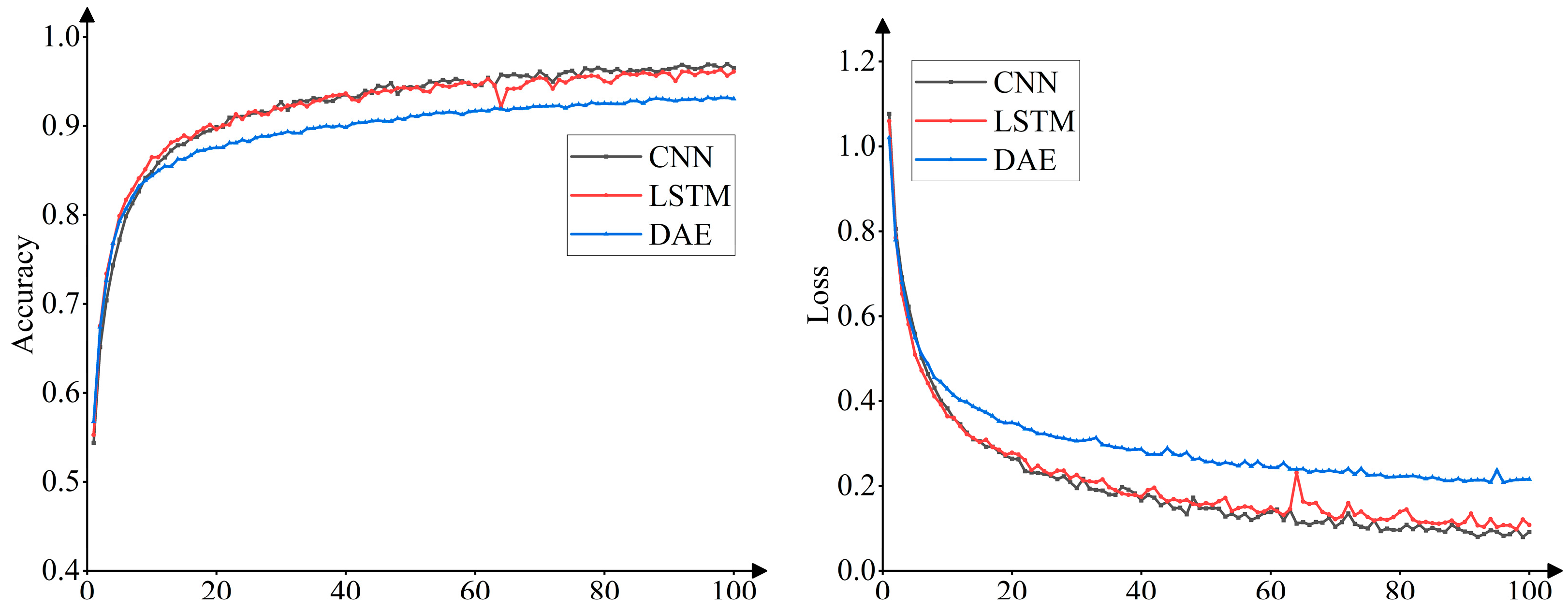
A total of 100 epochs are iteratively trained in this experiment, and Figure 8 shows the changes in accuracy and loss values during the training process. In Figure 8, with the increasing number of training iterations, the training curves of all three types of deep neural networks gradually reach convergence, and the final training accuracies of the CNN, LSTM, and DAE are 96.49%, 96.1%, and 93.03%.

4.3. Experimental Results

4.3.1. Evaluation Metrics

Evaluation metrics commonly used in damage classification problems include precision, recall, and F1-score, which are defined as follows:
P r e c i s i o n   =   T P T P   +   F P ,
R e c a l l   =   T P T P   +   F N ,
F 1   =   2   ×   P r e c i s i o n   ×   R e c a l l P r e c i s i o n   +   R e c a l l .
The precision indicates how many of the samples predicted to be in the damage category are correct, the recall indicates how many damage samples are correctly predicted, and the F1-score is the summed average of these two.

4.3.2. Experimental Results

Table 4 shows the test results of the three types of deep neural networks. With only three feature dimensions retained, the recognition accuracy of all three types of deep neural networks exceeds 93%, with the CNN having the highest recognition accuracy of 94.89%. The experimental results show that deep neural networks are still very good at recognising damage based on structural vibration signals when only selecting the feature dimension that accounts for 3.2% of the frequency statistics dataset after using sliding windows to extract modal frequencies and discarding many features with invalid damage information.
The confusion matrix for the CNN is shown in Table 5. As seen in Table 5, the CNN has high recognition accuracy for all six types of data, especially for the normal and Damage 5 types of data, with the highest F1-scores of 97.93% and 96.94%, respectively. Even for the Damage 1 type of data, which has relatively low recognition accuracy, the precision, recall, and F1-score exceed 92% when tested.

4.4. Experimental Comparison and Analysis

4.4.1. Influence of Feature Extraction Methods

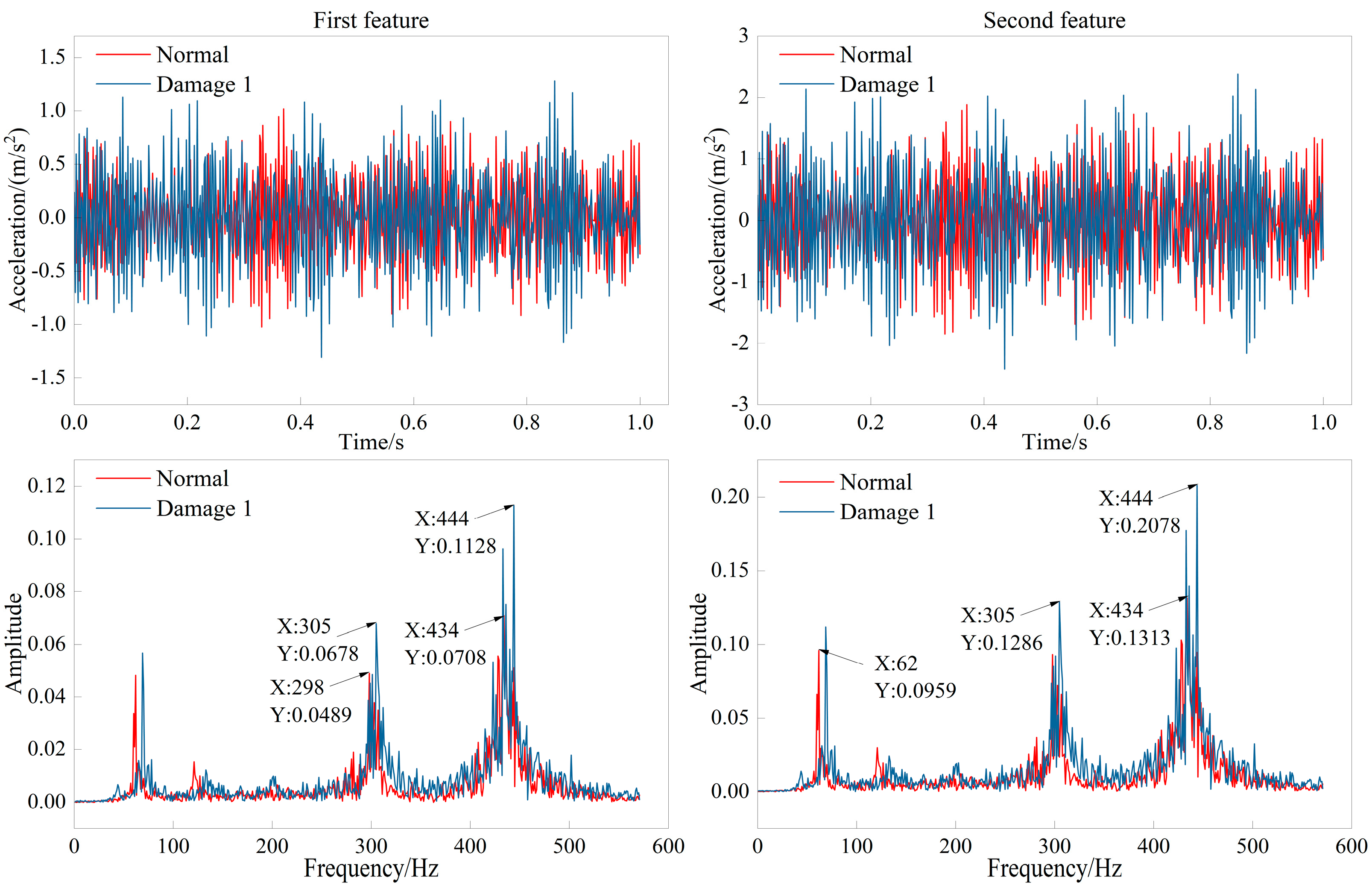
To analyse the validity of the modal frequency features, this paper also uses the extreme and mean values most commonly used in previous studies as feature representatives for time domain analysis for experimental comparison. Firstly, the maximum, minimum, and mean values are extracted for each sampling point using the same size sliding window and shift step as in the Fast Fourier Transform for feature extraction; secondly, the PCA is used for dimensionality reduction; and finally, the same model is used for training and the best model is retained using the five-fold cross-validation method. Table 6 shows the damage identification results. Compared to our proposed method, the recognition accuracy of the method using time-domain features on the three deep neural networks decreased by 4.96%, 3.04%, and 4.33%, respectively, indicating that the information extracted from the spectrograms did characterise the deeper damage class differences in the data.

4.4.2. Influence of Feature Selection Methods

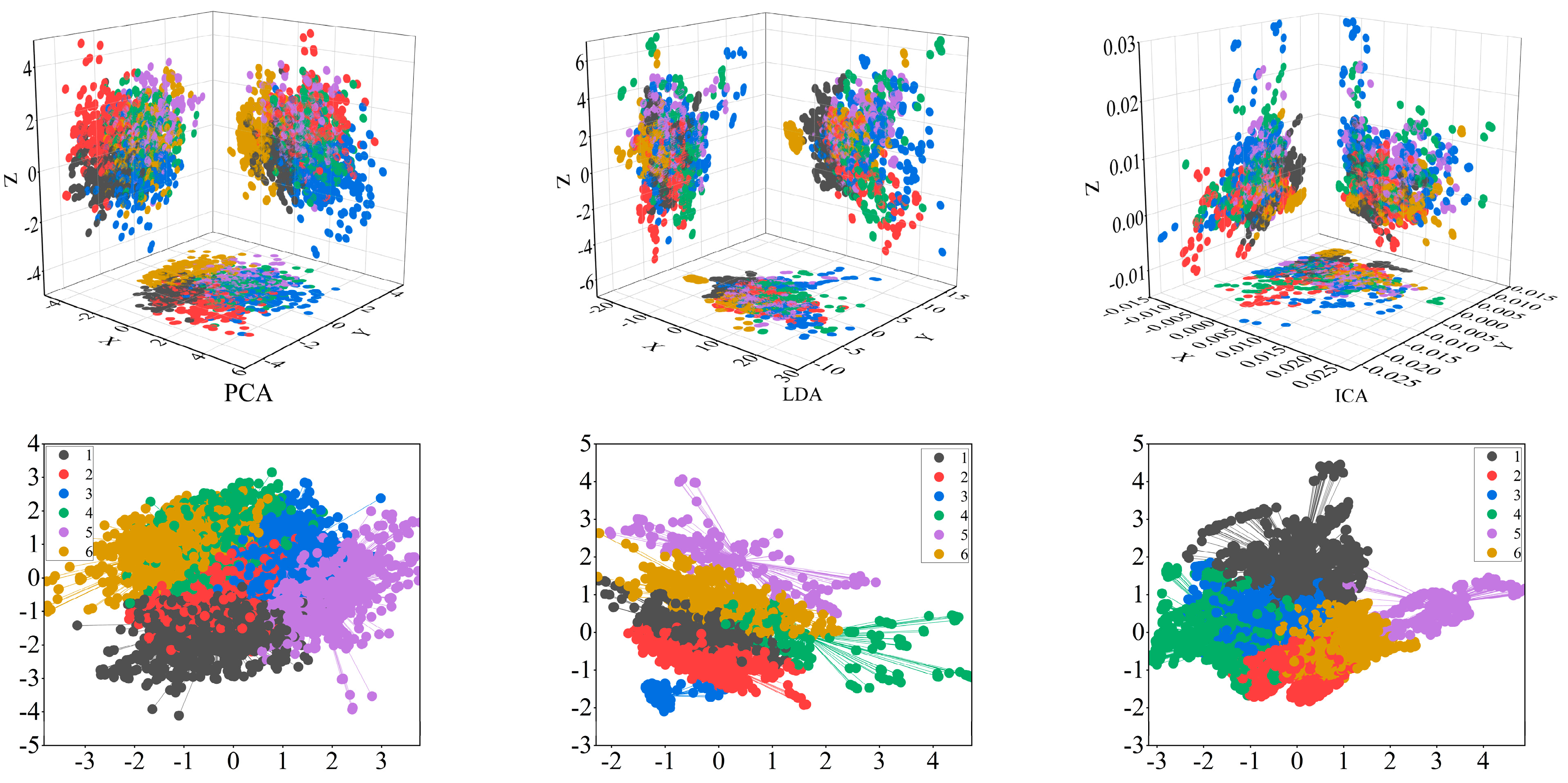
This paper also validates the effectiveness of PCA by investigating the impact of correlation and damage identification on data classification using two methods, linear discriminant analysis (LDA) and independent component analysis (ICA), respectively. Figure 9 shows the correlation distribution of data categories after processing using these three methods. Compared to these two methods, PCA reduces the dimensionality of the data while maintaining maximum differentiability through variance maximisation, effectively retaining information about the data categories, while the category distribution is generally consistent with the results obtained using the k-means clustering algorithm. Finally, using the same model, the damage recognition accuracy of PCA is also higher than the other two methods, and the results are shown in Table 7.
Only the first three features are selected for data downscaling using PCA, and the vast majority of features are discarded, so the effect of different feature dimensions on damage identification is investigated, as shown in Table 8. As the feature dimensionality increases, the recognition accuracy improves only slightly, the complexity of the model gradually increases exponentially, and the model starts to overfit. In contrast, our method achieves high accuracy in damage identification while keeping the computational effort to a minimum.

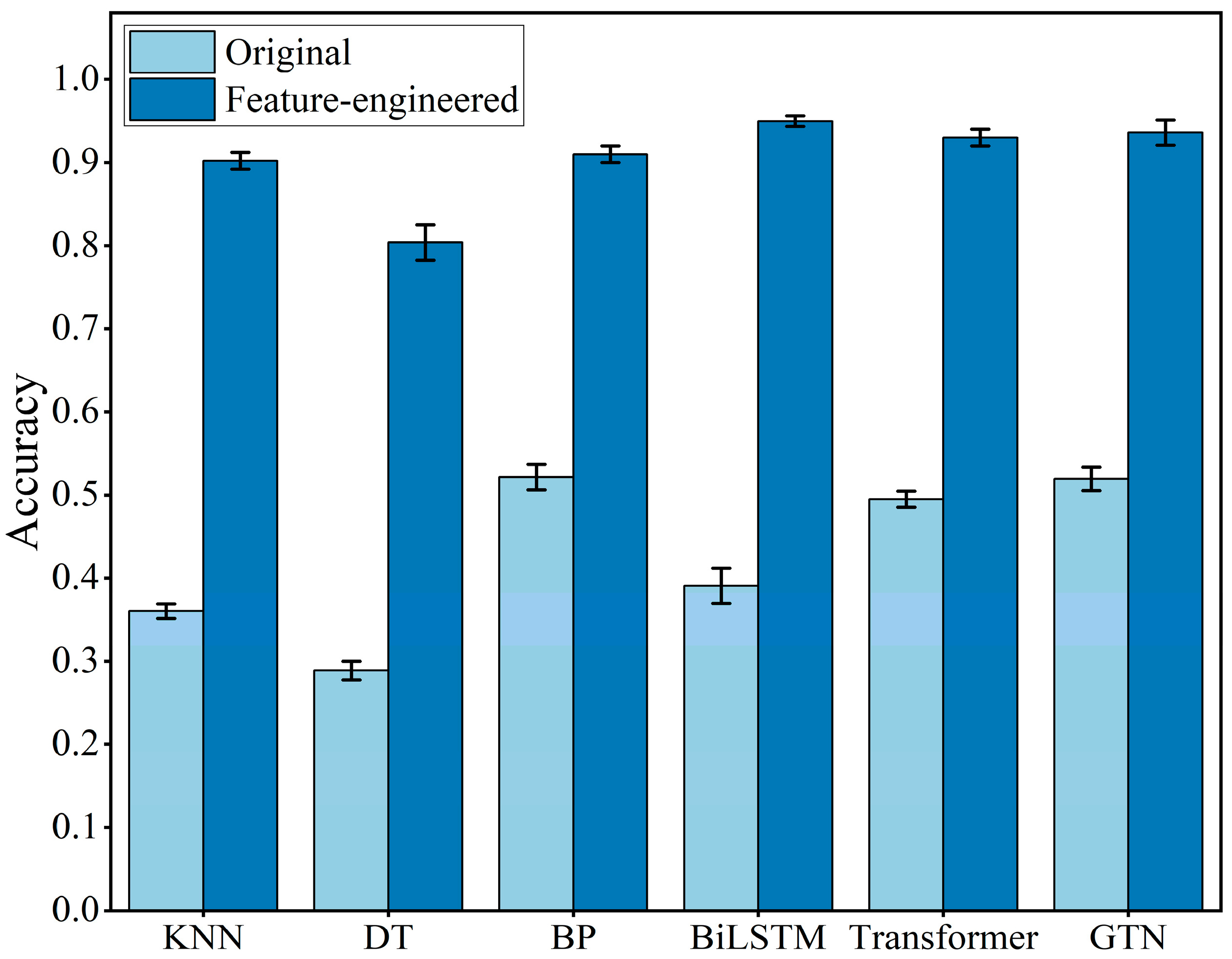
4.4.3. Influence of Different Algorithms

This paper uses other algorithms for comparison on the original dataset and the feature-engineered dataset, respectively, including KNN [31], DT [32], BP [33], BiLSTM [34], Transformer [35], and GTN [36]. For the machine learning algorithms, accuracy improvement is used as the objective function, and its hyperparameters are tuned through the Bayesian optimisation method in the fetch space by continuous iteration. The Transformer and GTN model architectures are both adopted from the original paper, and other relevant settings are used as described in this paper. Figure 10 shows the damage identification results. The recognition accuracy of the various algorithms is greatly improved on the feature-engineered dataset, which validates the effectiveness of our proposed feature engineering.

4.4.4. Influence of the Various Components in Feature Engineering

To investigate in detail the impact of the various aspects of feature engineering on the performance of damage identification, three different datasets are prepared, including the original dataset, the PCA-only dataset, and the fusion dataset, which is obtained by combining the PCA-only dataset with the feature-engineered dataset in the feature direction and by downsampling. In this paper, a shared model with parameters in the source and target domains is used to achieve transfer learning on the three datasets, thereby improving training speed and learning accuracy. Specifically, the pre-trained model based on the previous section is retrained on each of the three datasets. First, freezing the feature extraction layer of the model and training the fully connected layer near the output for 50 epochs to adapt it to the feature distribution in the new dataset, and then unfreezing it and fine-tuning the entire model architecture for 100 epochs. The initial learning rate is adjusted to 0.0001 for both stages, and other relevant settings are described in this paper; the test results are shown in Table 9.
Apart from the feature-engineered dataset, the fusion dataset performs relatively well because it contains not only the most original information but also the information after feature extraction and integration. The other two datasets both have lower recognition accuracy due to the inconspicuous distribution of the original features. This indicates that the modal frequency features extracted from the spectrograms in the damage feature extraction process greatly improve the sensitivity and accuracy of recognition.

4.5. Generalization Capability

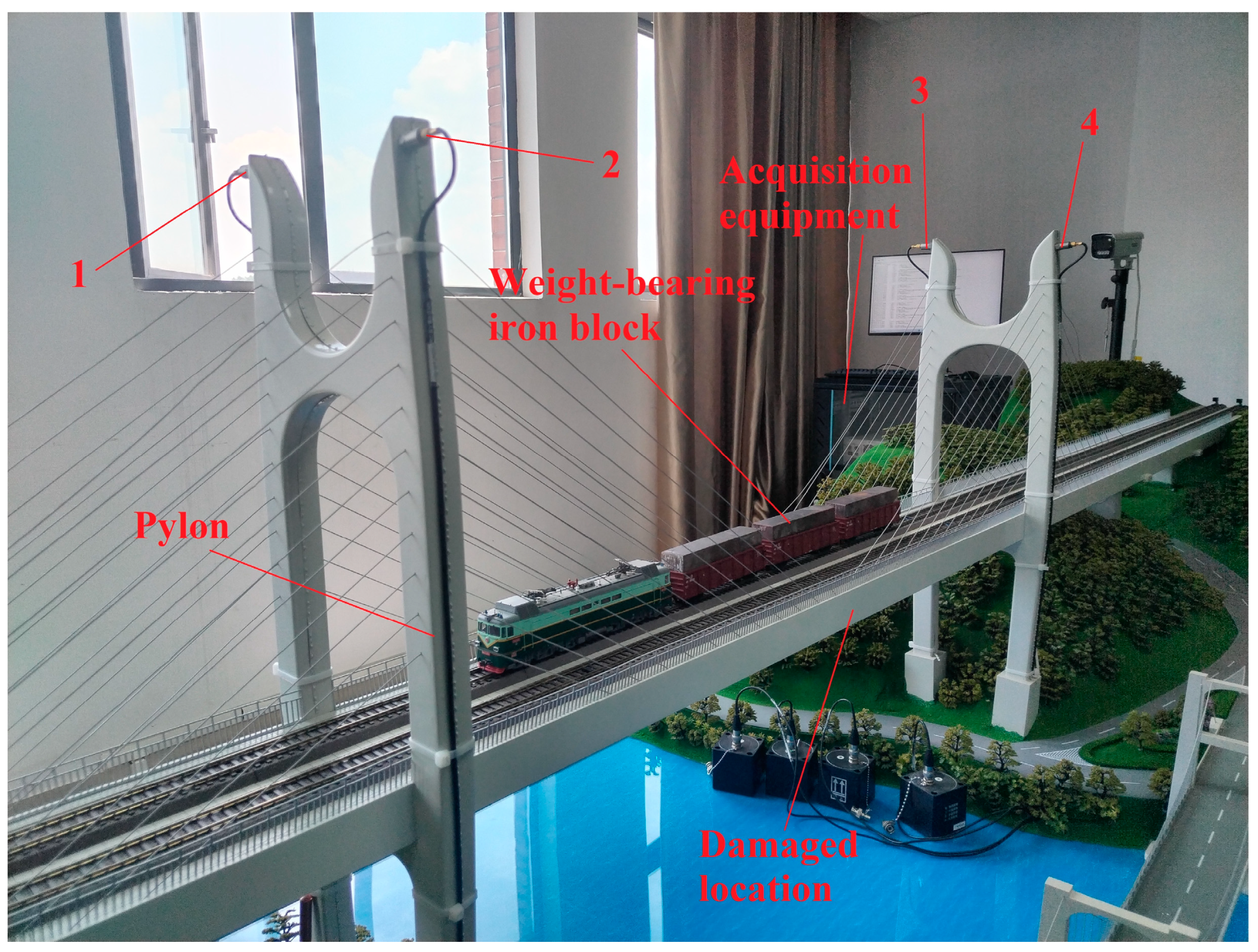
To show the generalisation capability of the recognition method based on the combination of data mining and deep neural networks, a bridge model is built in this paper and acquisition equipment such as sensors are arranged to obtain a monitoring dataset by collecting data in real-time. The dataset is the change data of vibration acceleration of the bridge when passing through the vehicle, the bridge structure and data acquisition equipment are shown in Figure 11.
The bridge as a whole is a cable-stayed bridge structure with a length of 5.1 m, and its cross-section is a uniform rectangle with a cross-section of 0.14   m × 0.04   m . To simulate the damage of the bridge, we artificially damage a rectangular skeleton base plate with a size of 0.13   m × 0.11   m in the shape of a metre at the bottom of the beams in the centre position of the two pylons. The vehicle is operated at a uniform speed of 0.13   m / s , on which six loaded iron blocks with a total mass of 3.6 kg are placed as vehicle loads, and four acceleration sensors on the bridges are mounted at the very top of both sides of the two pylons, with a sampling frequency of 1024 Hz. Through the experimental measurements, we obtain a dataset with a size of 24,000 × 4 , which consisted of 19,118 normal data and 4882 abnormal data.
Our proposed data pre-processing approach is applied to this dataset, while features are extracted in the frequency domain and downscaled by PCA; finally, the same model is used for experimental analysis. 
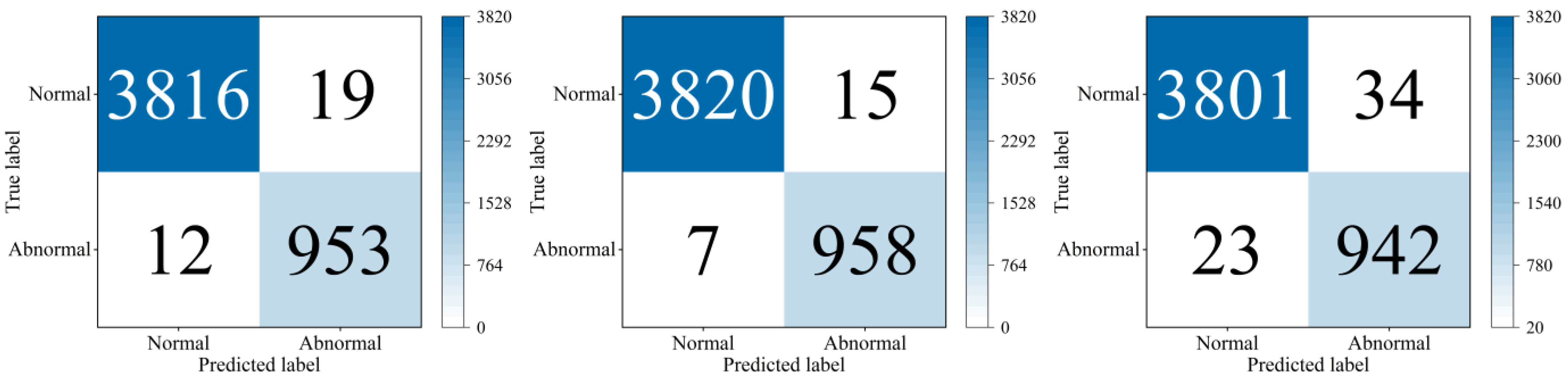
Figure 12 shows the confusion matrix for the three types of deep neural networks when tested.
As seen in the results, the detection accuracy of all three types of deep neural networks reaches over 98%, indicating that the trained deep neural networks can also give suitable outputs when our proposed method is applied to abnormal data detection.

5. Conclusions

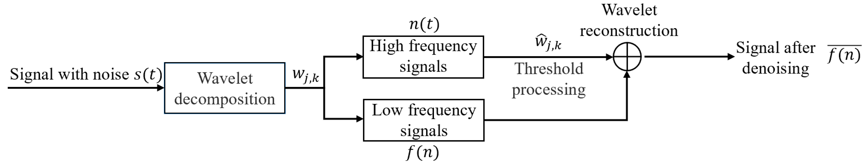
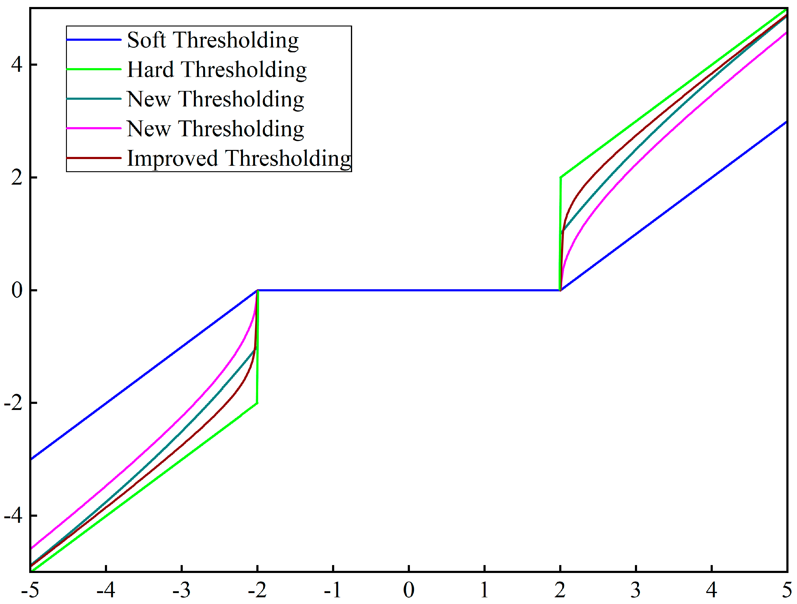
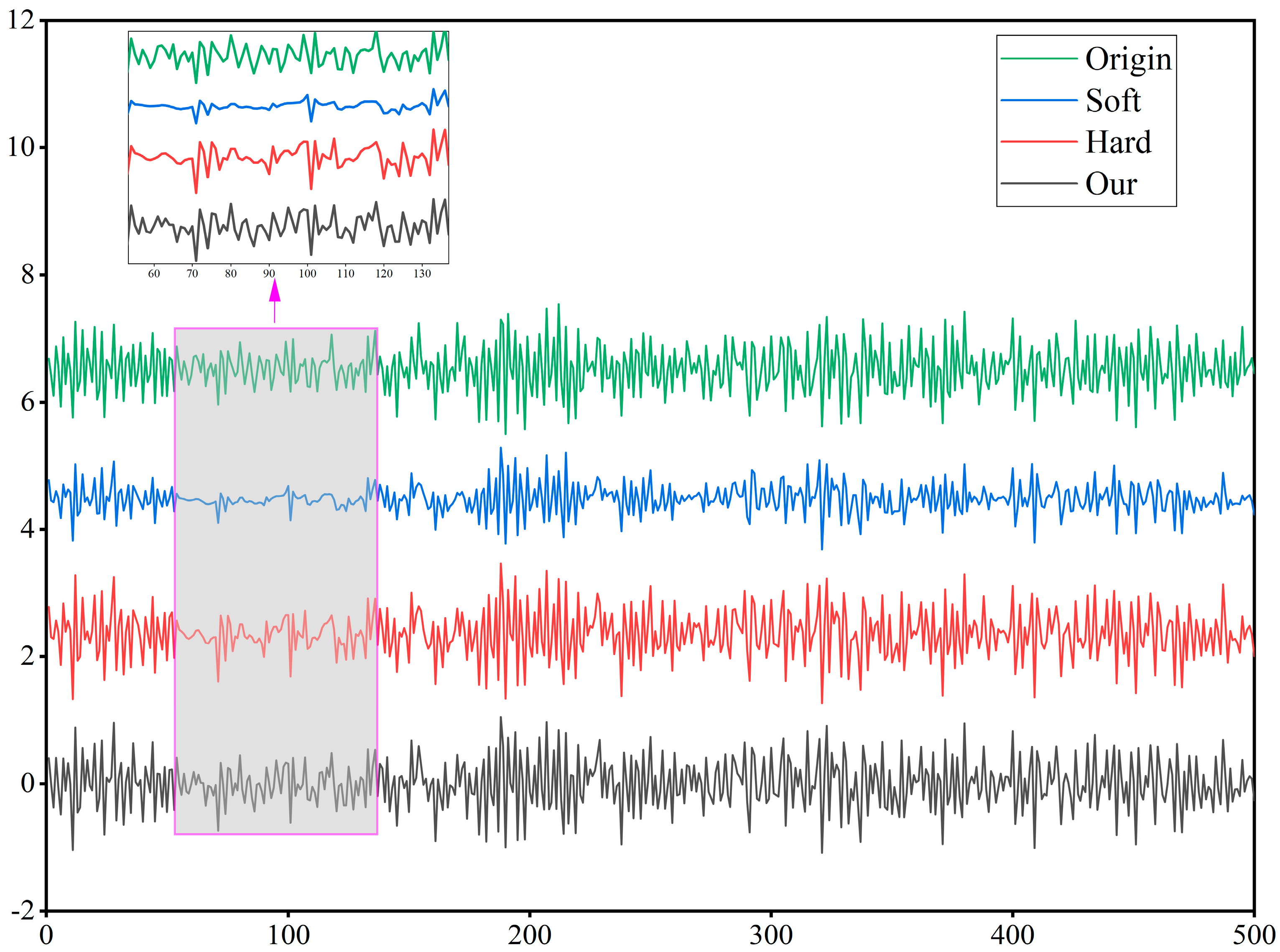
Based on structural vibration data and deep neural networks, this paper investigates data pre-processing, feature engineering, and damage identification techniques in the field of bridge health monitoring. Firstly, for the problem of noise interference in the original data, a wavelet threshold decomposition method based on parameter optimisationoptimisation is proposed, which effectively overcomes the discontinuity of the hard threshold function and the constant deviation of the wavelet coefficients in the soft threshold function by introducing two adjusting parameters in the threshold function to adapt to the different number of wavelet decomposition layers.
On the basis of this, to reflect the damage characteristics of the bridge structure, an in-depth analysis of the feature differences reflected in the signal spectrograms is carried out, and a feature extraction method based on the Fast Fourier Transform and sliding window extraction of modal frequencies and a feature selection method based on PCA are proposed so as to excavate the key information of the damage categories contained in the data. Finally, different deep neural networks are applied to identify the damaged data, the role of different feature engineering and data dimensions in damage identification is discussed, and the effectiveness of our method is verified by transfer learning.
The experimental results show that, compared with the original acceleration response, the new damage metrics effectively retain the information of the data categories and improve recognition ability and computational efficiency. Under the premise of retaining only three feature dimensions, the recognition performance and generalisation ability of the deep neural networks are extremely good, and their recognition accuracy on the test set exceeds 93%, with the highest F1-score of 97.93%. Therefore, our damage identification scheme achieves high recognition accuracy with minimal computational effort, has the ability to identify large amounts of monitoring data, and has the potential to be applied to real bridges.

Author Contributions

Conceptualization, Y.H. and X.Z.; Data curation, S.Z.; Investigation, S.Q. and S.W.; Methodology, Y.H.; Project administration, S.Q.; Software, X.L. and S.Z.; Supervision, X.Z.; Validation, S.Q. and X.Z.; Visualization, S.Q.; Writing—original draft, Y.H.; Writing—review & editing, S.W. All authors have read and agreed to the published version of the manuscript.

Funding

This research was funded by the National Key Research and Development Program of China (2020YFB1713300), and the Guizhou international science and technology cooperation base project: Guizhou optoelectronic information and intelligent application International Joint Research Center (Qiankehe platform talents No. 5802[2019]).

Data Availability Statement

No new data were created or analyzed in this study. Data sharing is not applicable to this article.

Conflicts of Interest

The authors declare no conflict of interest.

References

  1. Xu, Y.; Bao, Y.; Chen, J.; Zuo, W.; Li, H. Surface fatigue crack identification in steel box girder of bridges by a deep fusion convolutional neural network based on consumer-grade camera images. Struct. Health Monit. 2019, 18, 653–674. [Google Scholar] [CrossRef]
  2. Sun, L.; Shang, Z.; Xia, Y.; Bhowmick, S.; Nagarajaiah, S. Review of bridge structural health monitoring aided by big data and artificial intelligence: From condition assessment to damage detection. J. Struct. Eng. 2020, 146, 04020073. [Google Scholar] [CrossRef]
  3. Yi, T.-H.; Huang, H.-B.; Li, H.-N. Development of sensor validation methodologies for structural health monitoring: A comprehensive review. Measurement 2017, 109, 200–214. [Google Scholar] [CrossRef]
  4. Zhang, L.; Sun, L.; Shang, Z. Real-time reliability assessment based on acceleration monitoring for bridge. Sci. China Technol. Sci. 2016, 59, 1294–1304. [Google Scholar] [CrossRef]
  5. Mattson, S.G.; Pandit, S.M. Statistical moments of autoregressive model residuals for damage localisation. Mech. Syst. Signal Process. 2006, 20, 627–645. [Google Scholar] [CrossRef]
  6. Fan, W.; Qiao, P. Vibration-based damage identification methods: A review and comparative study. Struct. Health Monit. 2011, 10, 83–111. [Google Scholar] [CrossRef]
  7. Moughty, J.J.; Casas, J.R. A state of the art review of modal-based damage detection in bridges: Development, challenges, and solutions. Appl. Sci. 2017, 7, 510. [Google Scholar] [CrossRef]
  8. Hester, D.; González, A. A wavelet-based damage detection algorithm based on bridge acceleration response to a vehicle. Mech. Syst. Signal Process. 2012, 28, 145–166. [Google Scholar] [CrossRef]
  9. Roveri, N.; Carcaterra, A. Damage detection in structures under traveling loads by Hilbert–Huang transform. Mech. Syst. Signal Process. 2012, 28, 128–144. [Google Scholar] [CrossRef]
  10. Shahsavari, V.; Chouinard, L.; Bastien, J. Wavelet-based analysis of mode shapes for statistical detection and localization of damage in beams using likelihood ratio test. Eng. Struct. 2017, 132, 494–507. [Google Scholar] [CrossRef]
  11. Suarez, E.; Benavent-Climent, A.; Molina-Conde, R.; Gallego, A. Wavelet energy ratio index for health monitoring of hysteretic dampers. Struct. Control Health Monit. 2018, 25, e2071. [Google Scholar] [CrossRef]
  12. Kang, F.; Li, J.; Dai, J. Prediction of long-term temperature effect in structural health monitoring of concrete dams using support vector machines with Jaya optimizer and salp swarm algorithms. Adv. Eng. Softw. 2019, 131, 60–76. [Google Scholar] [CrossRef]
  13. Chandola, V.; Banerjee, A.; Kumar, V. Anomaly detection: A survey. ACM Comput. Surv. (CSUR) 2009, 41, 1–58. [Google Scholar] [CrossRef]
  14. Worden, K.; Manson, G. The application of machine learning to structural health monitoring, Philosophical Transactions of the Royal Society A: Mathematical. Phys. Eng. Sci. 2007, 365, 515–537. [Google Scholar] [CrossRef]
  15. Hajializadeh, D. Deep learning-based indirect bridge damage identification system. Struct. Health Monit. 2022, 22, 897–912. [Google Scholar] [CrossRef]
  16. Goodfellow, S.D.; Goodwin, A.; Greer, R.; Laussen, P.C.; Mazwi, M.; Eytan, D. Atrial fibrillation classification using step-by-step machine learning. Biomed. Phys. Eng. Express 2018, 4, 045005. [Google Scholar] [CrossRef]
  17. Chalapathy, R.; Chawla, S. Deep learning for anomaly detection: A survey. arXiv 2019, arXiv:1901.03407. [Google Scholar] [CrossRef]
  18. Bao, Y.; Tang, Z.; Li, H.; Zhang, Y. Computer vision and deep learning–based data anomaly detection method for structural health monitoring. Struct. Health Monit. 2019, 18, 401–421. [Google Scholar] [CrossRef]
  19. Liu, Z.; Cao, Y.; Wang, Y.; Wang, W. Computer vision-based concrete crack detection using u-net fully convolutional networks. Autom. Constr. 2019, 104, 129–139. [Google Scholar] [CrossRef]
  20. Parisi, F.; Mangini, A.; Fanti, M.; Adam, J.M. Automated location of steel truss bridge damage using machine learning and raw strain sensor data. Autom. Constr. 2022, 138, 104249. [Google Scholar] [CrossRef]
  21. Lipton, Z.C.; Kale, D.C.; Elkan, C.; Wetzel, R. Learning to diagnose with LSTM recurrent neural networks. arXiv 2015, arXiv:1511.03677. [Google Scholar] [CrossRef]
  22. Pathirage, C.S.N.; Li, J.; Li, L.; Hao, H.; Liu, W.; Ni, P. Structural damage identification based on autoencoder neural networks and deep learning. Eng. Struct. 2018, 172, 13–28. [Google Scholar] [CrossRef]
  23. Zheng, Z. Research and Application of Bridge Health Detection Based on Time-Frequency Analysis. Master’s Thesis, Chang’an University, Xi’an, China, 2019. [Google Scholar] [CrossRef]
  24. Wang, Y.; Zhu, G.; Wang, Z.; Wang, Z.; Wang, Y.; Yang, Q.; Gong, J. Research on white noise interference suppression of gis partial discharge online monitoring based on improved wavelet threshold. High Volt. Appar. 2019, 3, 37–43. [Google Scholar]
  25. Yang, E. Research on Multi-Source Heterogeneous Information Analysis and Data Fusion of Bridge Monitoring. Master’s Thesis, Yunnan University, Kunming, China, 2021. [Google Scholar] [CrossRef]
  26. Li, G. Research on Key Technologies of Bridge Health Monitoring Data Analysis Based on Deep Learning. Master’s Thesis, Chongqing Jiaotong University, Chongqing, China, 2018. [Google Scholar]
  27. Zhang, Y.; Lei, Y. Data anomaly detection of bridge structures using convolutional neural network based on structural vibration signals. Symmetry 2021, 13, 1186. [Google Scholar] [CrossRef]
  28. Kullaa, J. Distinguishing between sensor fault, structural damage, and environmental or operational effects in structural health monitoring. Mech. Syst. Signal Process. 2011, 25, 2976–2989. [Google Scholar] [CrossRef]
  29. Sun, W.; Wang, C. Power signal denoising based on improved soft threshold wavelet packet network. J. Nav. Univ. Eng. 2019, 4, 79–82. [Google Scholar]
  30. Liu, C.; Ma, L.; Pan, J.; Ma, Z. Pd signal denoising by joint vmd and improved wavelet threshold. Mod. Electron. Technol. 2021, 44, 45–50. [Google Scholar] [CrossRef]
  31. Feng, K.; González, A.; Casero, M. A kNN algorithm for locating and quantifying stiffness loss in a bridge from the forced vibration due to a truck crossing at low speed. Mech. Syst. Signal Process. 2021, 154, 107599. [Google Scholar] [CrossRef]
  32. Li, S.; Zuo, X.; Li, Z. Applying deep learning to continuous bridge deflection detected by fiber optic gyroscope for damage detection. Sensors 2020, 20, 911. [Google Scholar] [CrossRef]
  33. Zoubir, H.; Rguig, M.; Aroussi, M.E. Concrete Bridge defects identification and localization based on classification deep convolutional neural networks and transfer learning. Remote Sens. 2022, 14, 4882. [Google Scholar] [CrossRef]
  34. Mousavi, M.; Gandomi, H.A. Structural health monitoring under environmental and operational variations using MCD prediction error. J. Sound Vib. 2021, 512, 116370. [Google Scholar] [CrossRef]
  35. Katrompas, A.; Ntakouris, T.; Metsis, V. Recurrence and Self-Attention vs the Transformer for Time-Series Classification: A Comparative Study. In International Conference on Artificial Intelligence in Medicine; Springer International Publishing: Cham, Switzerland, 2022; pp. 99–109. [Google Scholar] [CrossRef]
  36. Liu, M.; Ren, S.; Ma, S. Gated transformer networks for multivariate time series classification. arXiv 2021, arXiv:2103.14438. [Google Scholar] [CrossRef]
Figure 1. Schematic diagram of wavelet threshold decomposition.
Electronics 12 03613 g001
Figure 2. CNN.
Figure 2. CNN.
Electronics 12 03613 g002
Figure 3. Data distribution.
Electronics 12 03613 g003
Figure 4. Threshold function. The dark cyan and magenta lines are threshold functions from references [29] and [30], respectively.
Electronics 12 03613 g004
Figure 5. Noise reduction comparison chart.
Electronics 12 03613 g005
Figure 6. Time domain and frequency domain comparison chart.
Electronics 12 03613 g006
Figure 7. Contribution of the principal components of each feature. The horizontal axis represents the 94 feature dimensions of the dataset, and the vertical axis represents the contribution of each feature component as well as the cumulative contribution, respectively.
Electronics 12 03613 g007
Figure 8. Changes in accuracy and loss values during training.
Electronics 12 03613 g008
Figure 9. Class correlation distribution for true and k-means cluster analysis. From left to right, the results of PCA, LDA and ICA analyses.
Electronics 12 03613 g009
Figure 10. Test results for different algorithms.
Electronics 12 03613 g010
Figure 11. Bridge structure and data acquisition equipment. The installation locations of the four sensors in the bridge are labelled using the numbers 1, 2, 3 and 4.
Electronics 12 03613 g011
Figure 12. Confusion matrix. From left to right, the test results for CNN, LSTM and DAE.
Electronics 12 03613 g012
Table 1. Selection of wavelet basis.
Wavelet Basisdb1db2db3db4db5db6db7db8
SNR20.89021.65820.91421.79521.63020.28420.96421.670
MSE0.0120.0100.0120.0100.0100.0140.0120.010
Table 2. Noise reduction assessment results.
Threshold FunctionsHard Threshold FunctionSoft Threshold FunctionOurs
SNR14.914813.314118.9289
MSE0.04970.07200.0194
Table 3. The setting of experimental parameters.
Optimisation AlgorithmLearning RateBeat1Beat2Decay RateBatch
Adam0.0010.90.99910−8128
Table 4. Test results of the three types of deep neural networks.
Evaluation MetricsPrecisionRecallF1-ScoreAccuracy
CNN94.87%94.88%94.87%94.89%
LSTM94.68%94.67%94.67%94.66%
DAE93.34%93.23%93.28%93.19%
Table 5. Confusion matrix for CNN.
Predicted Label
NormalDamage 1Damage 2Damage 3Damage 4Damage 5
Normal116043043
Damage 15110917191117
Damage 2114108917292
TrueDamage 31444101140192
labelDamage 411192619103413
Damage 541132181187
Total119512011148119711151224
Precision97.07%92.34%94.86%95.24%92.74%96.98%
Recall98.81%94.14%94.53%92.76%92.16%96.90%
F1-score97.93%92.23%94.69%93.98%92.45%96.94%
Table 6. Test results for different features.
MethodsCNNLSTMDAEFormer 3D Contribution
Time-domain features89.93%91.62%88.86%85.03%
Frequency features94.89%94.66%93.19%86.10%
Table 7. Test results for different dimensionality reduction methods.
MethodsCNNLSTMDAEFormer 3D Contribution
LDA87.06%85.31%80.11%84.64%
ICA87.70%86.95%87.45%-
Table 8. Results for different feature dimensions.
Feature Dimensions6912151821
CNN95.79%96.85%97.18%97.39%97.52%96.91%
LSTM94.52%95.48%96.19%97.15%96.87%96.30%
DAE94.66%94.70%95.29%94.77%95.50%95.36%
GFLOPs/GFLOPs(3-dim)CNN2.09103.08054.17155.16116.25217.2416
GFLOPs/GFLOPs(3-dim)LSTM234567
GFLOPs/GFLOPs(3-dim)DAE2.00883.02744.05575.09366.14137.1987
Table 9. Influence of various aspects of feature engineering on damage identification.
Different TreatmentsOriginalPCA-OnlyFusionFeature-Engineered
CNN48.51%31.96%60.36%94.89%
LSTM41.06%31.54%59.31%94.66%
DAE53.93%31.62%58.76%93.19%
Disclaimer/Publisher’s Note: The statements, opinions and data contained in all publications are solely those of the individual author(s) and contributor(s) and not of MDPI and/or the editor(s). MDPI and/or the editor(s) disclaim responsibility for any injury to people or property resulting from any ideas, methods, instructions or products referred to in the content.

