Abstract
The translation of traffic flow data into images for the purposes of classification in machine learning tasks has been extensively explored in recent years. However, the method of translation has a significant impact on the success of such attempts. In 2019, a method called DeepInsight was developed to translate genetic information into images. It was then adopted in 2021 for the purpose of translating network traffic into images, allowing the retention of semantic data about the relationships between features, in a model called MAGNETO. In this paper, we explore and extend this research, using the MAGNETO algorithm on three new intrusion detection datasets—CICDDoS2019, 5G-NIDD, and BOT-IoT—and also extend this method into the realm of multiclass classification tasks using first a One versus Rest model, followed by a full multiclass classification task, using multiple new classifiers for comparison against the CNNs implemented by the original MAGNETO model. We have also undertaken comparative experiments on the original MAGNETO datasets, CICIDS17, KDD99, and UNSW-NB15, as well as a comparison for other state-of-the-art models using the NSL-KDD dataset. The results show that the MAGNETO algorithm and the DeepInsight translation method, without the use of data augmentation, offer a significant boost to accuracy when classifying network traffic data. Our research also shows the effectiveness of Decision Tree and Random Forest classifiers on this type of data. Further research into the potential for real-time execution is needed to explore the possibilities for extending this method of translation into real-world scenarios.
1. Introduction
Network ubiquity has revolutionized the modern world and made it possible to connect to anyone anywhere, instantly. However, this ubiquity is a double-edged sword—not all communication is made in good faith, and a family of exploits known as (Distributed) Denial of Service ((D)DoS) attacks have plagued the time and minds of network engineers and administrators for decades. These types of attacks exploit the general lack of centralized control systems [1]. Traditionally, an expert in this area of cybersecurity is required to fortify, defend, and mitigate these attacks individually, but modern advancements in the area of machine learning have allowed researchers to alleviate the high need for domain experts in this task. As such, the most important task in this domain is now the accuracy of machine learning classifiers on the current intrusion detection datasets, a task made more difficult due to the imbalance of classes within these datasets. The vast majority of traffic across a network is benign, regular packets sent as part of a working system, with only a small number of these representing malicious packets and attacks. Highly accurate detection and classification of network attacks is required, as false alarms can lead to congestion in the network as relevant packets are discarded. Naive over- and undersampling is the traditional approach and although this can create balance in the dataset, it has the limitation of potential overfitting. For example, SMOTE—Synthetic Minority Oversampling Technique [2]—offers the ability to sample within the feature space. Other novel approaches have also been presented as the default methods for augmentation used by researchers when they need to balance a dataset, including methods like ADASYN, which relies on weighting the minority samples based on the difficulty of learning the data type [3], and RFMSE, which combines Minority SMOTE and Edited Nearest Neighbor (ENN) and was introduced for medical samples [4]. Although a significant improvement over traditional methods, due to their ignorance of general data location during synthesis, unwanted noise is introduced in the process. In comparison, the MAGNETO model (iMage-based Gan-enhanced convolutional NEural neTwOrk) introduced in [5], proposes a new type of image translation which preserves the relationships and semantic information of the different features. Instead of mapping features to pixels left to right, top to bottom, as many proposed systems do, Andresini et al. import a method of 2D mapping introduced in [6] for mapping gene expressions into images. This alternative mapping method groups similar features into neighboring pixels, allowing the spatial representation to encode information about more than just the order in which the features appear in the file. This allows the preservation of semantic relationships between the pixels/data points. Our research shows that even without the assistance of an augmentation model to balance the data, the DeepInsight method of data-to-image translation results in high accuracy and precision in classifying traffic data. We also demonstrate that there are advantages to using older and more established classifiers like Decision Trees and Random Forest models, in place of the original Convolutional Neural Networks (CNNs) from the MAGNETO model.
Our specific contributions to the area are as follows:
- To confirm the feasibility of the DeepInsight method for modern traffic data, using the implementation from [5] to keep our model’s fidelity to the original method.
- We introduce two new classifier types to examine if the Convolutional Neural Network (CNN) implemented in MAGNETO is the best model when using multiclass classification. For this, we implement a Decision Tree (DT) and a Random Forest (RF) classifier model.
- We extend the work conducted on the original datasets, such that we examine the results of using these datasets on both the original architecture and on the new Decision Tree and Random Forest classifiers.
- We extend the work conducted in [5] into new domains, using more recent and up-to-date datasets. Specifically, the CICDDoS 2019, 5G-NIDD, and BOT-IoT datasets, all made available for research purposes in the last five years.
- We apply the different models to the NSL-KDD dataset for the purposes of comparison to existing state-of-the-art models.
- We add a multiclass classification task to the model, using the original MAGNETO model in a One versus Rest classification task. For this, we split each dataset into files based on the different types of attacks and run training and testing over these files.
- We implement a full multiclass classification task by redeveloping the classifiers used in the MAGNETO model to operate on the new datasets with multiple attack types.
- We present a full comparison of our new versions of the DeepInsight method with new classifiers against several state-of-the-art models.
- We explore the overall execution time of the different classifiers within the MAGNETO experiments, both in the original paper and on our own computer architecture.
This paper is organized as follows: Section 2 goes over similar and related research in translating traffic data into images. Section 3 covers the methodology we used in this research and the reasons we used these specific implementations. It also covers and explains the MAGNETO model, as introduced in Andresini et al. [5]. Section 4 explains the process by which we processed the data for use in the experiments, and the details of different datasets we employed.Section 5 explores the results we achieved in the different classification tasks and the different classifiers we implemented, as well as thoroughly examines the execution time for the tasks and the accuracy, F1-score, recall, and precision of our DT and RF models against other state-of-the-art models. Finally, Section 6 underlines the conclusions from our work and outlines the potential for future research in this area.
2. Related Works
The research in this paper is based on the original experiments in [5] and the original DeepInsight method from [6]. Similar works have been published, with researchers looking to find the most efficient ways of using traffic-to-image translation for anomaly detection.
2.1. Using Images for Anomaly Detection
Work using traffic-to-image translation has been performed both with and without the use of machine learning models. This has led to tools like those introduced in [7], called NetViewer, which can display network traffic as images, in addition to detecting anomalies. Unlike the research in this paper, the authors do not make use of machine learning but instead offer “motion prediction” to detect anomalies using changes in the images. NetViewer allows the user to detect attacks visually, showing DDoS attacks, for example, as vertical lines within the image for the source/destination data. NetViewer creates different images based on different features, unlike DeepInsight, which combines the features to create a single image.
Further work to enable network administrators to view network traffic visually has been undertaken in papers such as [8]. The authors use the transformation of network traffic data into images to enable better detection of attacks and suspicious traffic. The authors use passive monitoring on both KREONet2 (KREONet2 is South Korea’s dedicated research and science network—Korea Research Environment Open Network 2), and on the University of Southern California network. The authors use packet header data to generate visual images of the network traffic. Image generation is conducted by bytes, working from left to right, top to bottom, meaning the semantic information between data points is not preserved in the way that it is in the DeepInsight model. The appearance of solid horizontal lines in images is again indicative of anomalies in the traffic data. The authors also make use of color to further offer differentiation of patterns in the images in real time. This is another differentiation from the MAGNETO model, which operates in greyscale.
2.2. Machine Learning for Image Data Classification
In general terms, much of the research into translating network traffic data into images for classification by neural networks has used the structure of the data to inform the ordering of pixels in an image. As such, changing the order of columns provides an entirely new image. This is the issue the DeepInsight translation method seeks to address.
In the current research landscape, many other researchers have developed methods of translation, many of which use the ordering of the files. In [9], the authors propose translating traffic data into images for classification by a Convolutional Neural Network for the purpose of detecting Botnet traffic and attacks. In this paper, the authors use a three-step process for taking the raw traffic data and turning them into images for use in the CNN. First, the data are split into sections which become either PCAP or binary files. Then, the data are processed, with the MAC and IP addresses anonymized and any empty data or duplicates discarded. Finally, the remaining data are transformed into images using grayscale pixels, with any data of shorter length being padded by white pixels. The addition of white space padding is a very visually significant difference from the DeepInsight method of translation. We have compared the results from Taheri et al. in our state-of-the-art comparison (see Section 5.6).
Similarly to [9], in [10] the authors use a Convolutional Neural Network (CNN) to classify traffic flow data that have been transformed into images, though their paper does not focus on anomaly detection or network intrusion. Their model, Seq2Img, utilizes a Reproducing Kernel Hilbert Space Embedding (RKHS) to convert the traffic data into images, as seen in Figure 1, which was created from Instagram traffic. Unlike [9] or [5], the images generated for Seq2Img are not grayscale. The use of RKHS embedding allows Seq2Img to take the dynamic behavior of the packets into account when generating the image, which provides extra detail and information for training the CNN. The process creates six-channel images, which are fed into the CNN for training and classification purposes. The CNN in Seq2Img classifies the image based on the application type the traffic flow is for, such as Facebook or Instagram. The Seq2Img model achieved a classification accuracy on the transformed traffic data of 88.42% using the RHKS embedding images.
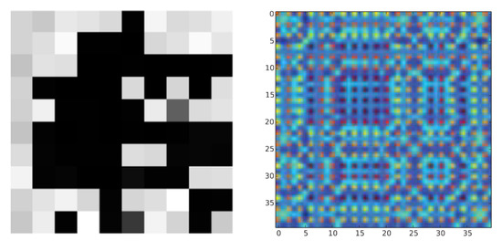
Figure 1.
An image generated by the DeepInsight method from Andresini et al. (2021) [5] (left (Reprinted with permission from Ref. 1385536-1, 2021, Elsevier), compared to an RKHS Embedding Image of Instagram traffic, from Chen et al. (2017) [10] (Reprinted with permission from Ref. 5606331016579, 2017, IEEE.) (right).
Regular, unencrypted network traffic is not the only type to be processed and classified in this way. In [11], the authors transform and classify encrypted traffic passed through VPNs. The images of the network traffic are used to train their CNN to recognize encrypted network traffic, using the ISCX VPN-non-VPN dataset [12]. The ISCX dataset has 14 types of encrypted traffic, 7 types of conventionally encrypted traffic, and 7 types of VPN encrypted traffic. Each session was processed into a series of images. Each byte of the traffic data was represented as an integer from 0 to 255, and thus transformed into a grayscale pixel. The resulting images were 28 × 28 pixels in size, and any data that were shorter than the total of 784 bytes was padded with zeroes. Longer data were truncated at 784 bytes. When classifying the images, the CNN model reached an F1-Score of 97.73% on the traditional encrypted traffic and 99.55% on the VPN encrypted traffic, demonstrating the effectiveness of traffic-to-image translation for classification purposes. A similar experiment was undertaken in [13], in which a CNN was used to distinguish images of network traffic that had been encrypted via different methods. The images, referred to as FlowPics, were generated from network traffic flow data in the ISCX dataset, and the classification of encryption type was achieved with an accuracy of 99.7%.
Other research has focused on detecting malware through the translation of network traffic flow data into image sequences. In [14], the authors translate Android malware network flow data into two-dimensional continuous image sequences for classification with a bidirectional Long Short-Term Memory (LSTM) model. Each packet is transformed into a 2D grayscale image for classification. The system, called Falcon, achieves 97.16% accuracy in detecting malware, and further achieves 88.32% accuracy in categorizing said malware.
3. Methodology
For the purposes of this paper, we have forgone the use of the AC-GAN as utilized in the original paper. This is to ensure we are able to examine the usefulness of the DeepInsight translation method on network traffic data alone, without the aid of an AC-GAN augmenting rare classes. All results were achieved on unaugmented datasets, and compared using multiple classifiers. We utilized the CNN and 2D CNN models from the original MAGNETO model and also implemented a Decision Tree and a Random Forest Classifier model for multiclass classification tasks. Future research could involve the use of the GAN implementation, forgoing it in these experiments to allow the demonstration of the DeepInsight method, as well as decreasing the needed computational power, as dedicated terminals such as those used to run training of a GAN on this scale were unavailable to us at this time. Figure 2 shows an abstracted overview of the MAGNETO model presented in Andresini et al. [5].
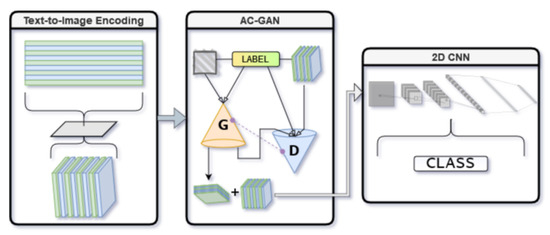
Figure 2.
An overview of the original MAGNETO model architecture using the methodology from [5], starting with the DeepInsight translation method, moving to the AC-GAN to balance the datasets, and finally the 2D CNN to classify the data.
The datasets used in this paper were transformed from network traffic data, in both .csv and .pcap files, into 10 × 10 images using the DeepInsight method. Prior to using the DeepInsight method, the dataset contains the following features:
- A 1D feature vector containing M features X1,…, Xm with each feature describing an independent characteristic of a network flow.
- A 1D class column vector containing categorical data of the names of each attack.
- A training set consisting of X, an NxM matrix containing training samples on rows with the 1D feature vector on the columns. Furthermore, the corresponding Y, an N x 1 vector which classifies each row to a particular class. (A binary label in the binary and One versus Rest classification tasks, and a multiple choice option in the multiclass classification task.)
DDoS datasets are famously imbalanced and thus true to life. Attacks are generally a small percentage of traffic on any real network, and an effective machine-learned model must be capable of working in an environment where access to balanced data is not possible. Section 5.5 specifies the exact distribution of the KDD’99 dataset over the 23 attack types. This dataset was used in the original paper, and again for our comparisons in Section 5.5. The pipeline from the original 2021 paper [5] has been utilized for this paper with a few small differences.
- Data pre-processing to ensure each dataset is of a valid form for future processes. This includes dropping any unnecessary columns of data which may result in overfitting, and the normalization of all features, encoded in the range [0,1]. The exception is the labels, which for the multiclass classification task are set to whole integers, and OneHotEncoded to provide a label matrix.
- Encoding training samples that consist of 1D vectors into a 2D form via t-SNE, wherein each training sample’s 2D form will be used to create an image. This is explained in Section 3.1.
- The training of the classifier model on the images created through the translation method. We have used four classifier models: a CNN, 2D CNN, Decision Tree, and a Random Forest classifier. The CNNs were used for all the classification tasks, whereas the DT and RF were used for the multiclass classification and the comparison tasks with both the original MAGNETO and other state-of-the-art models in a binary classification task.
As discussed above, for the purposes of our research, the use of the AC-GAN was omitted. We utilized the code provided by Andresini et al. [5], and kept the settings equal to the originals for the most part. As such, the training of the classifier occurred over 100 iterations with 2 epochs per iteration. In the CNNs, the settings for the dropout layers (of which there are two) and learning rate were chosen randomly in each iteration.The best model was originally saved when the accuracy achieved in that iteration was higher than the current saved best model. We altered this to rely on the F1-score instead, to improve overall performance. We also implemented two new classifiers, a Random Forest (RF) and a Decision Tree (DT) classifier, which provided high levels of accuracy and a high F1-score. The specifics of these implementations are discussed in Section 3.4.1 and Section 3.4.2, respectively.
3.1. Text-to-Image Encoding with DeepInsight
Normalization of the data was conducted using scikit-learn’s MinMax function. This was to ensure that all features have values in comparable ranges.
Each row from the dataset must be transformed into a form the classifiers can use. CNNs in particular place emphasis on pixel order and neighboring pixels, which means the use of a technique that can transform text while maintaining the semantic relationships between data points is of great importance.
To this end, we followed the example of both [6] and [5] in utilizing t-distributed Stochastic Neighbor Embedding (t-SNE) on the transposition of the dataset. Transposition is conducted so that each row contains traffic characteristics, with samples being the columns. t-SNE is a nonlinear technique that is particularly well suited for visualizing high-dimensional data. t-SNE maps high-dimensional data onto a two-dimensional space in a way that preserves local structure while also revealing global structures. Part of the t-SNE method constructs a probability distribution for each pair of flow characteristics from the training data and the similarity of each characteristic to is measured as a conditional probability that would have as its neighbor if neighbors were being picked in proportion to their probabilistic density under a -centered Gaussian. The operations also focus on minimizing the non-symmetric Kullback–Leibler divergence KL between distributions.
The non-symmetric Kullback–Leibler divergence is defined as:
where is the information gain achieved if P was used instead of Q.
The result is a dataset transformed from an MxN matrix to one of an Nx2 matrix where each row still represents the traffic characteristics and the two columns define 2D coordinates that can be used to visualize those characteristics as points on a Cartesian plane. This can be seen, abstracted, in Figure 3.
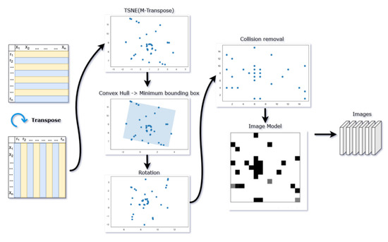
Figure 3.
The pipeline for the DeepInsight method of translating traffic flows into images.
In the next step, the Convex Hull Algorithm (CHA) is used to find the minimum bounding rectangle containing all points from the t-SNE transformation. A convex hull algorithm is an algorithm that takes a set of points in the plane and computes the convex hull of those points, in this case, the minimum bounding rectangle. Once found, the points are rotated to be horizontal or vertical, so that the images can be framed for the architecture of a Convolutional Neural Network. Finally, each point is assigned to a specific subsection of the image frame that most closely matches its point location from t-SNE.
The allocation of features to a pixel frame within the image can result in feature collision if more than one point finds itself within the same pixel frame. The method introduced in [5] introduced the use of Mutual Information (MI). This works to overcome the issues related to the method for addressing collisions in [6], which simply computed the average of values measured on heterogeneous characteristics. MI is invariant in feature space transformations such that where feature collisions occur, each is ranked based on their mutual information, and then the top feature is used for that frame. Figure 4 displays the methodology behing the Mutual Information collision resolution method introduced in Andresini et al. [5].
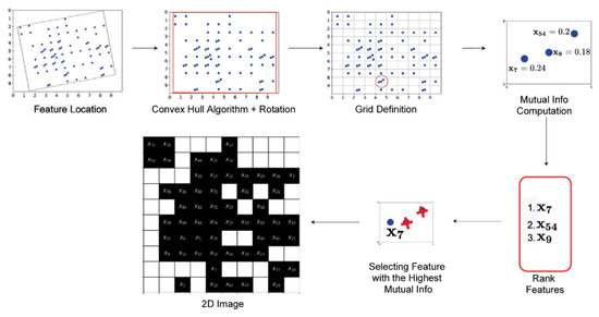
Figure 4.
The Mutual Information method introduced in Andresini et al., used to address collisions in the image space. From ([5], p. 112) ((Reprinted with permission from Ref. 1385536-1, 2021, Elsevier).
The end result of these steps is a blueprint, or scaffolding image, with each sample’s individual feature values being used as the grayscale values for the pixel frames. This results in each image having the same general structure; much like a species, a cat has a general structure shared between each breed.
The images we produced for human recognition were modified slightly in their production from the original MAGNETO paper. We utilized the Pillow image library, along with the previously implemented matplotlib, in order to create grayscale grid images with nine individual sample images in each. Labeled examples of this, showing the image and the attack label for the multiclass version of the dataset, can be seen in Figure 5.
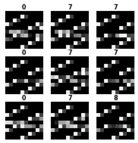
Figure 5.
A sample of nine images from the unaugmented, multiclass 5G-NIDD dataset, labeled with their attack classes.
3.2. Classification Using 2D Convolutional Neural Networks
For our experiments, the basic and 2D Convolutional Neural Network is trained to discriminate between the network flow classes, based on the image form of the samples. The primary reason researchers tend towards using a 2D CNN over approaches such as the Random Forest classifier is the ability to capture spatial contiguity in images. This is relevant to these experiments as the input data are encoded in such a way as to preserve feature relationships in 2D images. This model is a fully connected feed-forward neural network, with local filters and weight. There are three Conv2D layers alternating with Dropout layers-Conv2D layers are of sizes 32–64–128. Each Conv2D layer involves filter sets that replicate across the entire input, processing small local parts. Specifically, given an image p, the ith feature map for location (x, y) in a convolutional layer will be determined by a weight matrix and bias vector, along with a non-linear activation function:
where is the input patch centered at location (x, y) of the lth layer and ∗ represents the convolution function. The kernel is shared for each possible location (x, y), thus reducing the model complexity and making the network easier to train. Finally, it is flattened and goes through two dense layers of size. Note that there are no pooling layers as per [5]. The output layer’s activation function is sigmoid, for binary classification, and softmax for multiclass classification.
3.3. Multi-Class Classification with One versus Rest Tasks
A significant part of our experiments to expand the reach of the MAGNETO model involved the classification of multiple attack types, in addition to the traditional binary Benign/Malicious classification task. In order to conduct this while remaining as close to the original model as possible, a One versus Rest classification task was created. Each dataset was processed into a set of files, one for each attack type, containing all dataset samples, with each Label column containing a binary label indicating whether or not the sample was of that file’s class. In the case of the 5G-NIDD dataset, this meant splitting the dataset into eight attack types as well as one for Benign/Not Benign. The CICDDoS 2019 dataset contained eight attack types, whereas the BOT-IoT dataset contained 15. Each of these files was processed through the same methods as discussed in the previous section for the binary classification task. The algorithm was trained on each attack type through the corresponding dataset file and evaluated for effectiveness and accuracy. For this experiment, the original CNN models were the only classifiers used.
3.4. Multi-Class Classification with Full Dataset Processing
As a new and substantive extension of the original code for MAGNETO, we created a version that processed datasets with multiple potential attack labels. The different classes of attack were used for training as singular datasets with multiple potential labels, rather than the individual attack class datasets used in the One versus Rest task. Interestingly, the results for this task were significantly higher than the individually trained One versus Rest task. As we can see in the breakdowns of the different attack classes in each dataset (Table 1, Table 2 and Table 3), there are multiple rare classes which each have only a dozen or so instances in the set. This makes training the network model to recognize these classes exceptionally difficult. This puts severe restrictions on the level of accuracy that is possible when classifying these classes. The difference may also be related to the addition of two different classifiers for the multiclass classification task. As part of training this model, we moved away from the sole use of Convolutional Neural Networks (as used in [5]) and implemented both a Random Forest and a Decision Tree Classifier [15], to see if this had a significant effect on the accuracy of the multiclass classification of the dataset. The two new classifiers performed more effectively overall than the CNNs from Andresini et al. [5]. These results will be discussed in more detail in Section 5.

Table 1.
Breakdown of attack classes in the CICDDoS2019 dataset.
Table 2.
Breakdown of attack classes in the 5G-NIDD dataset.
Table 3.
Breakdown of attack classes in the Bot-IoT dataset.
In adapting the CNN models for the full multiclass classification task, we made only minor changes. The CNN models were set up in the same way as for binary classification, with the difference being the last layer using a softmax activation function, and with the number of outputs equal to the total number of attack classes.
3.4.1. Implementing the Random Forest Classifier
We implemented a Random Forest Classifier using scikit-learn’s library [15] and optimized it using a modified version of Andresini et al.’s hyperopt function. The number of trees, maximum depth, random state, and the criterion function were all chosen at random and tested for optimal results over the course of 150 iterations, with two epochs per iteration. The number of trees varied between 20 and 200, and the maximum depth was set between 2 and 10. Random state was set as either 32 or 42, and the criterion functions of gini, entropy, or log-loss were selected at random. The randomized nature of the RF model resulted in significant differences in execution time between runs, because of the maximum number of trees and depth.
3.4.2. Implementing the Decision Tree Classifier
The Decision Tree Classifier was implemented using the scikit-learn library [15], and optimization involved the choice of a random state. The settings for the DT model were primarily the default settings, with only the random state and depth being altered in the optimization phases. The classifier was again trained over 150 iterations and two epochs per iteration. This classifier offered the best performance in execution time, as discussed in Section 5.
3.5. Comparative Tasks
In order to adapt the overall comparisons to the limitations of our available computational power, we used the multiclass models, with a binary version of the datasets, for all classifiers. We also used the original datasets (CICIDS17, UNSW-NB15, and KDD99) from the Andresini et al. experiments, in order to compare these results on the original models to the newly implemented classifiers. We also performed these experiments on the NSL-KDD dataset to allow for better comparison against other state-of-the-art machine learning models for intrusion detection.
4. Datasets and Processing
In [5], the datasets used were the KDDCUP99 (found at http://kdd.ics.uci.edu/databases/kddcup99/kddcup99.html (accessed on 7 Janurary 2023)), UNSW-NB15 (found at https://research.unsw.edu.au/projects/unsw-nb15-dataset (accessed on 7 January 2023)), CICIDS17 (found at https://www.unb.ca/cic/datasets/ids-2017.html (accessed on 10 January 2023)), and AAGM17 (found at https://www.unb.ca/cic/datasets/android-adware.html, (accessed on 10 January 2023), and not used in our experiments) datasets. Our project introduced newer datasets, so as to examine the effect of the DeepInsight method on datasets more representative of the current landscape of threat detection. We provided comparisons between the original experiments and our results in Section 5.5.
We also undertook experiments to see how our multiclass version of MAGNETO, with the Random Forest and Decision Tree classifiers, performed against the original datasets, with the exception of the AAGM17 dataset, which was extremely computationally expensive. These results can also be found in Section 5.5.
The new datasets used in these experiments are CICDDOS2019, 5G-NIDD, and BoT-IoT. We performed an additional examination on the datasets used by Andresini et al. in [5]—KDD99 Cup, UNSW-NB15, and CICIDS17. They were all evaluated through the use of our modified MAGNETO algorithm to test the performance of our proposed approach, and particularly to offer a comparison between the original MAGNETO experiments and our modified classifiers. These were pre-processed for use in the experiments, as shown below. The previous set of datasets (KDD99 Cup, UNSW-NB15, and CICIDS17) as well as the benchmark dataset of NSL-KDD were used only in part. We selected a random sample set of 10% of each set for use in our experiments. The original MAGNETO experiments also used only a small selection of the sets, so this offered the best way to create a true comparison.
All our datasets, plus our full code and results are available for download for research purposes (code and results can be downloaded from https://github.com/aerynsfyre/MAGNETO-extended (updated on 29 July 2023), datasets as modified and the images generated and their datasets can be found at https://tinyurl.com/2p96uzye (updated on 29 July 2023)).
4.1. CICDDOS2019 Dataset
CICDDOS2019 contains both benign and up-to-date attacks from two broad categories—exploitation and reflection. The dataset was created to widen the scope of attacks available in research datasets while providing high-quality, true-to-real-world condition network flows. In total, eight attack classes are represented, including benign samples. CICDDOS2019 contains 50 million records across two days, which presents an extensive amount of data. The CICDDoS2019 dataset [16] requires processing prior to use with the MAGNETO model. First, there exist NA and infinite values in some records, and it is necessary to remove these rows. Secondly, features that may result in overfitting, such as Source and Destination IP, are dropped. The original dataset contains 87 features. In total, we dropped 49 unnecessary or potentially over-fitting features, resulting in a dataset with 38 features. Categorical features, such as the type of attack, RAS/EAS/Benign, are encoded using a LabelEncoder. The ultimate labeling system of the training data is 0 for Attack and 1 for Benign. Next, data normalization is performed with the use of sklearn’s MinMaxScaler.
The training and testing datasets were created utilizing Pandas Dataframes to enable random splits and shuffling of the data. The split of 20% testing data to 80% training data was conducted with a random selection. The full dataset was used in each of the experiments. The multiclass experiments were performed based on the “Label” feature, which gave eight separate attack classes, including “Benign”, as shown in the breakdown in Table 1.
4.2. 5G-NIDD Dataset
The 5G-NIDD Dataset is a 2022 dataset presented by Samarakoon et al. [17], offering a large sample of intrusion detection data from multiple sources collected over a 5G wireless network. The data, from the University of Oulu, Finland, were collected by a 5G testbed, and are fully labeled for use in machine learning research. Containing many types of attacks, the dataset provides an up-to-date and comprehensive set for testing. Rows containing NA or infinite values were removed, and categorical features were encoded with LabelEncoder. The values were normalized with the MinMaxScaler. Due to the number of attack types, we utilized a binary classification of Malicious/Benign, as per the labeling of the dataset. For the multi-class classification task, the feature “Attack Type” was used to separate the classes of attacks and benign traffic. This gave nine output classifications, including the “Benign” class for normal traffic. The breakdown of these classes is shown in Table 2.
4.3. BOT-IoT Dataset
The BOT-IoT dataset, from the University of New South Wales Canberra campus, captured traffic representing both normal and botnet traffic [18]. It contains DDoS, DoS, OS and Service Scan, Keylogging, and Data Exfiltration attack data types, offering a good opportunity for multi-class classification using MAGNETO’s One versus Rest task. For the binary classification challenge, we applied a filter of Attack/Benign to the dataset. Any rows with NaN or infinite values were dropped, whereas categorical features were encoded, and all values were normalized using the MinMaxScaler. The multiclass version, based on the “Label” feature, gave 15 attack classes, including “Benign”, as shown in the breakdown in Table 3.
4.4. KDD99 Cup Dataset
Introduced in 1999, the KDD99 Cup dataset was one of the first intrusion detection datasets for research [19]. In spite of its age, the KDD99 dataset is still widely used by machine learning and cybersecurity researchers. In 2015, the KDD99 dataset had been utilized in almost 150 studies, primarily for training machine learning IDS models [20]. The KDD99 dataset breakdown, with regards to the ratio of malicious/benign traffic and the number of redundant samples, is shown in Table 4. For the purposes of this study, we utilized 10% of the dataset, split into two sets—80% for training and 20% for testing.
Table 4.
Distribution of the KDD99 Cup dataset for attacks and their redundancy rates with regards to the original dataset records.
4.5. NSL-KDD
There have been numerous attempts to “clean” the KDD99 Cup dataset, especially with regards to its redundant records, shown in Table 4. The result of these attempts was the NSL-KDD dataset (The full NSL-KDD dataset can be found here: https://www.unb.ca/cic/datasets/nsl.html (accessed on 7 January 2023)) [21]. It utilizes the same sample set as the KDD99 dataset does, but it removes redundant or unnecessary records, making it more efficient for machine learning tasks like this one. We again utilized 10% of the dataset in our experiments.
4.6. CICIDS17 Dataset
The CICIDS17 dataset, or the Canadian Institute of Cybersecurity System dataset of 2017, has long been a standard training and testing set in machine learning for IDS. Because it was utilized in the original MAGNETO paper, we have reproduced that experiment here and trained a binary classification task for this dataset using our newly implemented Random Forest and Decision Tree classifiers. The randomly selected 10% of the samples selected were used for these experiments.
4.7. UNSW-NB15 Dataset
The UNSW-NB15 dataset was released for research purposes in 2015 [22,23]. It contains a large set with 49 features and nine attack types. The number of samples is also significant, as it contains 25,40,044 unique records. As such, using only a selection of the total samples is required for efficient computation [24]. We have used a random selection of 10% of the full set.
5. Results
5.1. Binary Results
The results for the Binary classification task can be seen in Table 5. The MAGNETO model provided high levels of accuracy, even without the addition of the GAN implementation to balance the datasets in use. The execution time, however, was significant for the CNN and 2D CNN models. For the binary task on the 5G-NIDD dataset, the full run of training and testing took 23 h, 42 min, and 39 s. The CICDDoS19 dataset completed its run in 1 h, 6 min, and 46 s, much faster than its rival. The BOT-IoT dataset completed training in 34 h, 37 min, and 9 s.
Table 5.
The results of the Binary classification task using the MAGNETO CNN model on the new datasets.
The original paper provided overall accuracy and the F1-score for the datasets used. As such, we cannot compare the original paper’s precision and recall against our own experiments. Nonetheless, we have provided the precision and recall for the binary classification task using the MAGNETO CNN implementations.
The initial results from the binary classification task used for the CICDDoS 2019 dataset provided a trained model with the first dropout layer at 0.09082176810268824, the second dropout layer set to 0.8144037383748151, with a learning rate of 0.0009158694003247323. This model achieved an F1-Score of 99.78%. Interestingly, the model had high recall but no precision. The Convolutional Neural Network model used for the binary classification task resulted in a very low precision in classification.
The best performance of the Binary Classification Task on the 5G-NIDD dataset was achieved with dropout layers of 0.041691190108933865 and 0.8349497093285286, and a learning rate of 0.0007422573800689679. This achieved a balanced accuracy score of 99.46% and an F1-Score of 99.45%.
The binary classification of the BOT-IoT dataset gave a best performance of 97.07% accuracy and 95.47% F1-score, several percentage points lower than the other two datasets. Dropout layer 1 was set at 0.004898578679374063, and dropout layer 2 was 0.6595608323069847, with a learning rate of 0.0006702515026435587.
The BOT-IoT dataset, when split along the lines of Malicious/Benign, contains more than 1.8 million records of benign data and almost 450,000 records of malicious data in the training set. The testing set contains just over 450,000 benign samples and approximately 111,000 malicious samples. This is distinctly imbalanced—somewhat more so than the other two datasets—and may account for the difference in accuracy once trained.
5.2. Multiclass One versus Rest Results
The results of the unaugmented One versus Rest multiclass classification task can be seen in Table 6, Table 7 and Table 8.
Table 6.
Results from the One versus Rest multiclass classification task on the unaugmented CICDDoS 2019 dataset.
Table 7.
The unaugmented 5G-NIDD dataset One versus Rest multiclass classification results by attack type.
Table 8.
Multiclass One versus Rest results for the unaugmented BOT-IoT dataset.
The results of the One versus Rest multiclass classification task on the full 5G-NIDD base station one dataset are shown according to Attack Type in Table 7. Because these are the unaugmented results, obtained without the use of the GAN module, we can see the low F1-Score on the rarest class-ICMPFlood, which only achieved an F1-Score of 49.977%. This is because, in the unaugmented dataset, there are only 929 samples of this attack class in the training set and 226 in the testing set, out of more than one million samples total.
The imbalance of the unaugmented BOT-IoT dataset meant that the results for the One versus Rest classification task were significantly lower than that of the other datasets. As shown in Table 8, the F1-Scores suffer in the rarer classes. In some of the rarest classes, only a few dozen samples are available to train the model on that type of attack, which results in a poor representation in the network.
5.3. Full Multiclass Classification
The results of training the model on the unaugmented full multiclass dataset were significantly higher than that of the One versus Rest task when using the Convolutional Neural Networks implemented by [5]. To explore this, we implemented two new classifiers, a Decision Tree and Random Forest model. The results shown in Table 9, Table 10 and Table 11 are the results of training on images size 10 × 10, using the best performing of these four classifiers, the Decision Tree model. In contrast to the high results of the DT and RF classifiers, the original CNN achieved an F1-score of 62.02% on the CICDDoS19 dataset, 14.49% on the BOT-IoT dataset, and 62.02% on the 5G-NIDD dataset. Likewise, the 2D CNN from [5] achieved an F1-score of 70.4% on the CICDDoS19 dataset, 55.36% on the BOT-IoT dataset, and 70.40% on the 5G-NIDD dataset. The most significant contrast was the original CNN on the BOT-IoT dataset, which performed significantly lower than the other classifiers on this dataset. This is likely due to the higher number of attack classes and the severe imbalance in data types. Full comparative results can be seen in Section 5.4, which shows that the Decision Tree classifier resulted in the best overall performance, closely followed by the Random Forest classifier.
Table 9.
Full multiclass classification task with the unaugmented CICDDoS19 dataset using the Decision Tree Classifier.
Table 10.
Full multiclass classification task with the unaugmented 5G-NIDD dataset using the Decision Tree Classifier.
Table 11.
Full multiclass classification task with the unaugmented BOT-IoT dataset using the Decision Tree Classifier.
Although the original CNN models appeared to be inferior in classifying multiclass images from the new datasets, the Decision Tree Classifier performed very well on the unaugmented datasets. Given the level of imbalance present in the dataset, the DT classifier displayed the effectiveness of these models in multiclass classification problems. The full results for the Decision Tree Classifier can be seen in Table 11. Comparing the results of the multiclass classification using the DT with the One versus Rest classification using the 2D CNN, we can see a significant improvement on the performance of the unaugmented dataset overall.
5.4. Classifier Comparison for Multiclass Task
Having extended the reach of the MAGNETO algorithm by adding a Random Forest and Decision Tree Classifier to the multiclass version of the task, we have provided a full comparison of the different classifier models. On the unaugmented datasets, this resulted in significantly different scores, with the Decision Tree Classifier coming out significantly ahead of the Convolutional Neural Network classifiers, and achieving results fairly close to those of the Random Forest classifier.
The full multiclass classification on the CNN, 2D CNN, Random Forest, and Decision Tree Classifier models was completed over 150 training iterations, with two epochs per iteration. The overall accuracy on the unaugmented datasets using the different classifiers can be seen in Figure 6, with F1-Score shown in Figure 7.
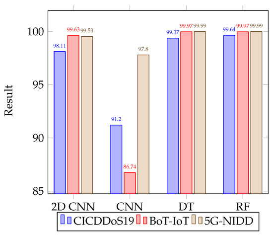
Figure 6.
Comparative results for accuracy of different classifiers for multiclass classification on the unaugmented datasets.
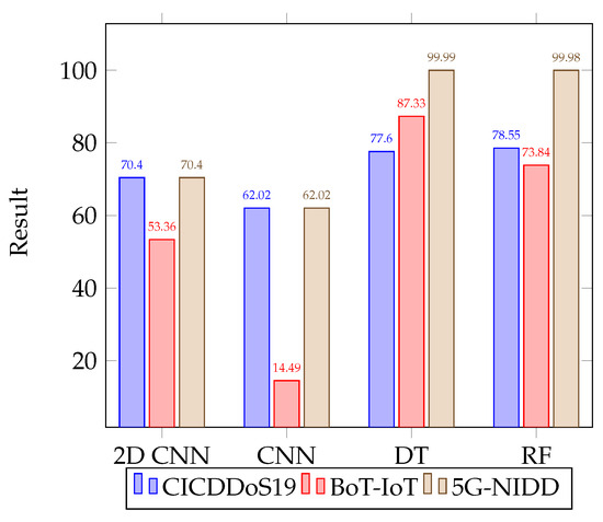
Figure 7.
Comparative results for F1-score using different classifiers for multiclass classification on the unaugmented datasets.
Settings for the Random Forest Classifier implemented were optimized with hyperopt and forests of up to 200 trees were used, with variable maximum depth between two and eight nodes. The different optimization functions were all utilized in random selection.
The Decision Tree Classifier switched between the random states of 32 and 48. A Support Vector Machine was considered, but discarded for the high computational complexity and time requirements associated with convergence on very large datasets.
When comparing the overall results of the multiclass classification task with the One versus Rest task, it can be seen in the differences between the latter two rows in Table 12 that the multiclass classification task with the Decision Tree classifier outperforms the One versus Rest task with the 2D CNN classifier. Therefore, our modified, multiclass version of MAGNETO proves more accurate in classifying the unaugmented datasets than the original version of MAGNETO.
Table 12.
Results from the different classification tasks using the MAGNETO model without the GAN implementation.
The overall results on the unaugmented datasets using the different classifiers show the effectiveness of the DeepInsight method. Even with multiclass classification and significantly imbalanced classes, the accuracy and F1-scores of the models were able to reach over 99% and 77% in the lowest scores, with the F1-score going as high as 99.98% on the 5G-NIDD dataset. The breakdown of the multiclass results shown for the Decision Tree Classifier displays the effectiveness of the translation method, as the individual classes achieve high scores in classification. We also display the Area Under the ROC Curve, or AUC value results for the different classifiers over the CICDDoS 2019 dataset in Figure 8. This shows relatively similar performance over the attack types, with the DT and RF classifiers still offering the best overall performance. In contrast, the AUC results for the 5G-NIDD dataset, shown in Figure 9, show that the DT and RF classifiers offered a significantly improved performance in comparison to the CNNs, as is also the case on the BOT-IoT dataset, as shown in Figure 10.
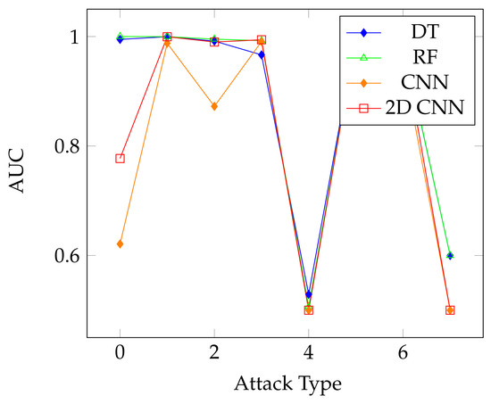
Figure 8.
Area under the ROC curve results for the classifiers using the CICDDoS 2019 dataset.
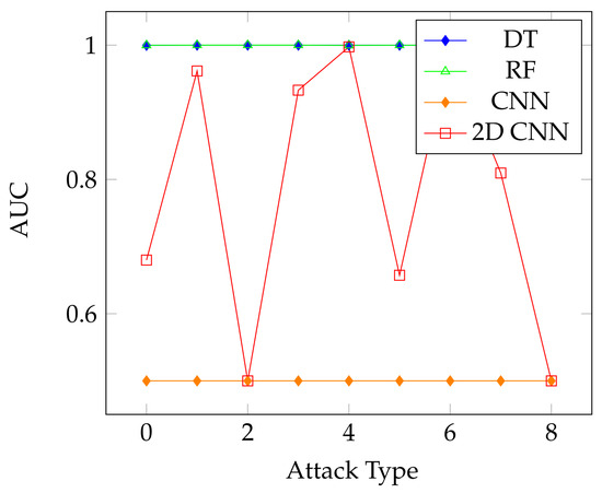
Figure 9.
Area under the ROC curve results for the classifiers using the 5G-NIDD dataset.
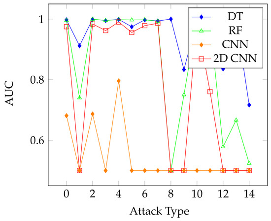
Figure 10.
Area under the ROC curve results for the classifiers using the BOT-IoT dataset.
5.5. Comparing Results with Andresini et al.
The results of the classifiers for the Andresini et al. paper can be seen in Table 13. These results are for the Binary classification task, using the original CNN. We have compared them to a new version of the binary classification task using our Random Forest and Decision Tree classifiers. Comparing the results from the original paper to the binary results from the new datasets show a significant difference, as seen in Table 12. In keeping with the original MAGNETO paper, only 10% of each dataset was used for these experiments. We have compared accuracy across the classifiers in Figure 11.
Table 13.
The results achieved by Andresini et al. [5] in their original binary classification task compared with the binary classification results from the new version of MAGNETO using the Random Forest and Decision Tree classifiers. The best results are highlighted for each dataset. (Reprinted with permission from Ref. 1385536-1, 2021, Elsevier).
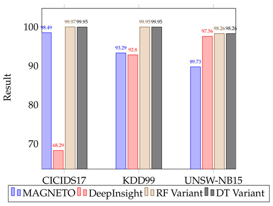
Figure 11.
Comparative results for accuracy of original and new classifiers for binary classification on the original datasets.
With regards to the new datasets, it is important to note that any comparison of the original datasets to these is only useful with the caveat that the results demonstrate the types of intrusion data on which the MAGNETO and DeepInsight methods are effective. It does, however, demonstrate the effectiveness of the MAGNETO model on more recent datasets, which are more representative of the current information flowing through devices.
The original datasets used in [5] were the KDD’99 Cup [19], UNSW-NB15, and the CICIDS17 [16]. We improved our ability to compare the different classifier models by performing binary classification on all of these datasets, with the exception of the AAGM17 dataset, which was excluded from the computational power required to process this dataset. Given the nature of the KDD99 dataset, as shown in Table 4, we also decided to run our models on the NSL-KDD dataset, which is an improved version of the KDD99 set, with redundant records and information removed. It is specifically designed for machine learning, and whereas Andresini et al. did not use this version of the dataset, several of the state-of-the-art classifiers we compared our models with did use the NSL-KDD set, and so we felt it reasonable to include these results. For further comparison, we also performed multiclass classification on the KDD99 dataset, using the newly implemented Decision Tree and Random Forest classifiers.
The results on the multiclass classification on two of the original datasets, as shown in Table 13, show the high accuracy and F1-scores achieved even across imbalanced datasets. The breakdown of the KDD99 dataset is shown in Table 14, so as to demonstrate how imbalanced the dataset is when using a multiclass classification model. Based on this breakdown, the overall results for our classifiers show significant promise for classifying malicious traffic. It is noted that the Random Forest classifier performs better on these datasets than the Decision Tree classifier, and further research is necessary to explore this trend. Some of the classes are so imbalanced that they appear only in single digits in the training set, and not at all in the testing set. This naturally brings the overall results of classification down with regard to F1-scores for the minority classes.
Table 14.
A breakdown of the different attack classes and the results of the multiclass classification task using the DT classifier in the KDD99 dataset.
It is also worth noting that the original paper by Andresini et al. [5] did not use the entirety of the datasets. The KDD99 dataset used was only 10% of the full training set. For CICIDS17, they used 100,000 samples in the training set and 900,000 samples in the testing set. For comparison and context, we have included the sizes of the original datasets in Table 15. For the purposes of comparison, we also utilized 10% of the datasets in this experiment. In comparison, all of the new datasets (CICDDoS19, BOT-IoT, and 5G-NIDD) were run using the entire dataset. Table 15 and Table 16 show our results in detail in comparison with the original results in Andresini et al. [5].
Table 15.
The full sizes of the original datasets used in Andresini et al. and their 10% sample sizes used in these experiments.
Table 16.
The multiclass classification results on the original datasets from Andresini et al. [5].
5.6. Comparing with State of the Art Models
To fully examine the effectiveness of the DeepInsight method and the MAGNETO model, we have compared our results using the DT and RF models with recent machine learning intrusion detection models. The results of this comparison can be found in Table 17. We only considered models introduced since 2022 and only machine learning-based IDS models. The comparison used our binary classification task on the NSL-KDD, KDD99, UNSW-NB15, and CICIDS17 datasets, using the newly implemented Decision Tree and Random Forest classifiers. These were chosen as they were the most common datasets used in this type of research, and as such would offer truly competitive results.
Table 17.
A comparison of current state-of-the-art IDS machine learning classifiers.
Our primary source for these state-of-the-art models was recent surveys into the area of machine learning for intrusion detection, including papers such as [29,30,31]. Of particular use was Maseer et al. [28], which provided benchmarks for the different models and datasets, current as of 2021. It provides benchmark results on the CICIDS17 dataset for both Decision Tree and Random Forest classifiers, allowing clear comparisons between these benchmarks and the results from this paper.
The model created by Hammad et al. [26] also utilizes the t-SNE algorithm, which is used in this paper. Their proposed model, t-SNERF, performs extremely well on the UNSW-NB15 dataset. Their model combines a stochastic k-nearest neighbor model and a Random Forest classifier. This offers suggestions for future research into using the DeepInsight method to classify network traffic. The implementation of the nearest neighbor scheme into MAGNETO may provide even higher accuracy. Another point of note is that the T-SNERF algorithm was implemented in R, whereas the MAGNETO algorithm used in this paper was implemented in Python. Creating a different implementation of MAGNETO in other programming languages is certainly an avenue for future research.
5.7. Execution Time
Concerning execution time, the full multiclass classification task over 150 epochs on the 5G-NIDD dataset took only 25 min and 35 s using the DT model. The BOT-IoT dataset took a significantly longer time to complete, taking 12 h, 55 min, and 29 s. This is still significantly less time than the CNN model achieved on the same dataset in the binary classification task over 100 epochs. The execution time for the CICDDoS19 dataset was 25 min and 35 s. These times suggest the extended execution time for the BOT-IoT dataset may have been an outlier, or caused by something within the dataset itself. The extra time could also be due to the randomized nature of each iteration. The depth of the Decision Tree is chosen from a set for each epoch, and deeper trees take longer to build and train. This is similar to the Random Forest classifier, which had a random number of trees between 5 and 200 per iteration, meaning the length of time for the execution would vary depending on the randomly selected number of trees in the forest.
Another important consideration with regard to the execution time is the fact that we did not have a dedicated machine for the experiments. As such, the execution time of the algorithm may have been affected by multiple unknown background processes. The longest execution times for all datasets were those for the CNN and 2D CNN models. For the purposes of accurate comparison, we ran several of the original datasets on the original CNN model implemented by Andresini et al., so as to provide data for a ratio between the time taken in the original experiments and the execution time in these experiments. We have included the NSL-KDD dataset in these experiments due to its use in the different state-of-the-art models in Section 5.6. Our results are visible in Table 18, where MAGNETO (original) displays the results from the original paper by Andresini et al., and MAGNETO (new) shows the results of that same model, using the original code, on our own architecture.
Table 18.
Comparative results for execution time in original and new classifiers for binary classification on the KDD99 and UNSW-NB15 datasets. “Andresini et al. [5]” refers to the original experiments for MAGNETO, whereas “[5] on our machines” refers to the same model and code run on our computer architecture. (Reprinted with permission from Ref. 1385536-1, 2021, Elsevier).
Looking at the sizes of the datasets in Table 15, we can see that the CICIDS17 dataset, even at 10% of its size, is significantly larger than the other original datasets. Given that this set has 2,197,863 samples in the 10% dataset, when compared to the smallest of the datasets, the NSL-KDD, which contains 18,118 samples in the 10% dataset, it is of little surprise that the execution time for the CICIDS17 dataset is significantly higher than the other sets.
Based on the results reported in Andresini et al. [5], we have created a comparative figure to show the different execution times. The original paper shows a very low execution time; however, when we used the original CNN models on the same datasets, our results were significantly different. Our only change was to use the softmax activation function. In order to give a reasonable and accurate comparison of the execution time of the different models, we ran the CNN models using the code from Andresini et al. [5] on the three original datasets to examine the difference our computer architecture made to the results.
In the original MAGNETO architecture, the KDD99 dataset took 38.6 min to complete 100 iterations. On our computers, the same algorithm and dataset took 84 min. Similarly, the UNSW-NB15 dataset in the original paper took 18.2 min. Using the same code, that dataset took 467 min and 50 s. This demonstrates a disparity between the resources available to us as opposed to those used by Andresini et al. [5]. Interestingly, the DT and RF classifiers still perform at a level comparable with that of the original papers, though the CNN models are greatly increased in computational time. Our implemented DT and RF models actually perform better, with regard to execution time, than the original models.
6. Conclusions and Future Research
The DeepInsight method of data-to-image translation shows great promise for machine learning in multiple disciplines. MAGNETO’s components, including the Mutual Info method of dealing with pixel collisions—even without the use of an AC-GAN to augment rare classes in the datasets—offer further refinements that provide a robust method of anomaly detection. The move from using the CNN models for multiclass classification tasks towards the use of Decision Tree Classifiers shows a very significant improvement in performance. Even in unaugmented datasets, the DT and RF models offered high levels of accuracy, precision, and recall.
Future research should explore the possibilities of running the MAGNETO algorithm in real time, as the computational power and time required to translate the datasets into images are not insignificant. Developing an implementation that can translate the data into images in real time is essential if the DeepInsight method and the MAGNETO model are to be used in anything more than academic research. The current and original implementations of the MAGNETO model involve generating all images for a given dataset at the outset of running the program and then undertaking training and testing. A new implementation that trains the model and then takes the testing data and translates each traffic flow sample into an image before classifying it individually would offer a way to time the algorithm to explore if it is possible to run it in real time. This implementation would therefore be of great use for further research.
Our experimental setup did not include the AC-GAN implemented by the original authors of [5], due to computational and time restraints. However, this is a feature to explore further in future research, and we plan to explore this aspect of the algorithm further in future papers.
Our research shows the effectiveness of the DeepInsight method of data-to-image translation and the usefulness of having the ability to preserve semantic data about the relationships between different data points in the dataset. Over all the different tasks, the MAGNETO model was highly successful in classifying the attack samples, especially with the implementation of different classifiers such as Decision Trees, whereas the original CNN classifier performed more poorly than expected when used for the full multiclass classification task, the implementation of other classifiers allowed us to demonstrate the overall effectiveness of this method of image translation.
Author Contributions
Conceptualization, A.D. (Adam Dunning) and A.D. (Aeryn Dunmore); methodology, A.D. (Aeryn Dunmore); software, A.D. (Aeryn Dunmore); validation, A.D. (Aeryn Dunmore); formal analysis, A.D. (Aeryn Dunmore); investigation, A.D. (Aeryn Dunmore); resources, J.J.-J., F.S. and J.K.; data curation, A.D. (Aeryn Dunmore) and J.J.-J.; writing—original draft preparation, A.D. (Aeryn Dunmore) and A.D. (Adam Dunning); writing—review and editing, A.D. (Aeryn Dunmore); visualization, A.D. (Aeryn Dunmore) and A.D. (Adam Dunning); supervision, J.J.-J.; project administration, J.J.-J.; funding acquisition, J.J.-J., F.S. and J.K. All authors have read and agreed to the published version of the manuscript.
Funding
The authors would like to thank the Ministry of Business, Innovation, and Employment (MBIE) from the New Zealand Government to support our work with the grant (MAUX1912) which made it possible for us to conduct the research.
Data Availability Statement
All our code files and results are available for download and use in future research at https://github.com/aerynsfyre/MAGNETO-extended (updated 29 July 2023). The dataset, with images generated using the MAGNETO DeepInsight method, can be found for download at https://tinyurl.com/2p96uzye (updated 29 July 2023).
Conflicts of Interest
The authors declare no conflict of interest. The funders had no role in the design of this study; in the collection, analyses, or interpretation of data; in the writing of the manuscript; or in the decision to publish the results.
Abbreviations
The following abbreviations are used in this manuscript:
| AC-GAN | Auxiliary Classifier Generative Adversarial Network |
| CICDDoS | Canadian Institute of Cybersecurity Distributed Denial of Service |
| CNN | Convolutional Neural Networks |
| DDoS | Distributed Denial of Service |
| DT | Decision Tree |
| ENN | Edited Nearest Neighbor |
| GAN | Generative Adversarial Networks |
| IP | Internet Protocol |
| KREONet 2 | Korea Research Environment Open Network 2 |
| LSTM | Long Short-Term Memory |
| MAGNETO | Image-based GAN-Enhanced Neural Network |
| MI | Mutual Information |
| PCAP | Packet Capture |
| RF | Random Forest |
| RKHS | Reproducing Kernel Hilbert Space Embedding |
| SMOTE | Synthetic Minority Oversampling Technique |
| t-SNE | t-distributed Stochastic Neighbor Embedding |
| VPN | Virtual Private Network |
References
- Brooks, R.R.; Yu, L.; Ozcelik, I.; Oakley, J.; Tusing, N. Distributed Denial of Service (DDoS): A History. IEEE Ann. Hist. Comput. 2022, 44, 44–54. [Google Scholar] [CrossRef]
- Chawla, N.V.; Bowyer, K.W.; Hall, L.O.; Kegelmeyer, W.P. SMOTE: Synthetic Minority Over-sampling Technique. J. Artif. Intell. Res. 2002, 16, 321–357. [Google Scholar] [CrossRef]
- He, H.; Bai, Y.; Garcia, E.A.; Li, S. ADASYN: Adaptive Synthetic Sampling Approach for Imbalanced Learning. In Proceedings of the 2008 IEEE International Joint Conference on Neural Networks (IEEE World Congress on Computational Intelligence), Hong Kong, China, 1–8 June 2008; pp. 1322–1328. [Google Scholar] [CrossRef]
- Xu, Z.; Shen, D.; Nie, T.; Kou, Y. A hybrid sampling algorithm combining M-SMOTE and ENN based on Random forest for medical imbalanced data. J. Biomed. Inform. 2020, 107, 103465. [Google Scholar] [CrossRef]
- Andresini, G.; Appice, A.; Rose, L.D.; Malerba, D. GAN augmentation to deal with imbalance in imaging-based intrusion detection. Future Gener. Comput. Syst. 2021, 123, 108–127. [Google Scholar] [CrossRef]
- Sharma, A.; Vans, E.; Shigemizu, D.; Boroevich, K.A.; Tsunoda, T. DeepInsight: A methodology to transform a non-image data to an image for convolution neural network architecture. Sci. Rep. 2019, 9, 11399. [Google Scholar] [CrossRef]
- Kim, S.S.; Reddy, A.L.N. A Study of Analyzing Network Traffic as Images in Real-Time. In Proceedings of the IEEE 24th Annual Joint Conference of the IEEE Computer and Communications Societies, Miami, FL, USA, 13–17 March 2005; Volume 3, pp. 2056–2067. [Google Scholar] [CrossRef]
- Kim, S.S.; Reddy, A.L.N. Modeling Network traffic as Images. In Proceedings of the IEEE International Conference on Communications, 2005, ICC 2005, Seoul, Republic of Korea, 16–20 May 2005; Volume 1, pp. 168–172. [Google Scholar] [CrossRef]
- Taheri, S.; Salem, M.; Yuan, J.S. Leveraging Image Representation of Network Traffic Data and Transfer Learning in Botnet Detection. Big Data Cogn. Comput. 2018, 2, 37. [Google Scholar] [CrossRef]
- Chen, Z.; He, K.; Li, J.; Geng, Y. SEQ2IMG: A Sequence-to-Image Based Approach Towards IP Traffic Classification Using Convolutional Neural Networks. In Proceedings of the 2017 IEEE International Conference on Big Data (Big Data), Boston, MA, USA, 11–14 December 2017; pp. 1271–1276. [Google Scholar] [CrossRef]
- He, Y.; Li, W. Image-based Encrypted Traffic Classification with Convolution Neural Networks. In Proceedings of the 2020 IEEE Fifth International Conference on Data Science in Cyberspace (DSC), Hong Kong, China, 27–29 July 2020; pp. 271–278. [Google Scholar] [CrossRef]
- Draper-Gil, G.; Lashkari, A.H.; Mamun, M.S.I.; Ghorbani, A.A. Characterization of Encrypted and VPN Traffic using Time-related Features. In Proceedings of the 2nd International Conference on Information Systems Security and Privacy, Rome, Italy, 19–21 November 2016; pp. 407–414. [Google Scholar] [CrossRef]
- Shapira, T.; Shavitt, Y. FlowPic: Encrypted Internet Traffic Classification is as Easy as Image Recognition. In Proceedings of the IEEE INFOCOM 2019—IEEE Conference on Computer Communications Workshops (INFOCOM WKSHPS), Paris, France, 29 April–2 May 2019; pp. 680–687. [Google Scholar] [CrossRef]
- Xu, P.; Eckert, C.; Zarras, A. hybrid-Falcon: Hybrid Pattern Malware Detection and Categorization with Network Traffic and Program Code. arXiv 2021, arXiv:2112.10035. [Google Scholar] [CrossRef]
- Pedregosa, F.; Varoquaux, G.; Gramfort, A.; Michel, V.; Thirion, B.; Grisel, O.; Blondel, M.; Prettenhofer, P.; Weiss, R.; Dubourg, V.; et al. Scikit-learn: Machine Learning in Python. J. Mach. Learn. Res. 2011, 12, 2825–2830. [Google Scholar]
- Sharafaldin, I.; Lashkari, A.H.; Hakak, S.; Ghorbani, A.A. Developing realistic distributed denial of service (DDoS) attack dataset and taxonomy. In Proceedings of the 2019 International Carnahan Conference on Security Technology (ICCST), IEEE, Chennai, India, 1–3 October 2019; pp. 1–8. [Google Scholar]
- Samarakoon, S.; Siriwardhana, Y.; Porambage, P.; Liyanage, M.; Chang, S.Y.; Kim, J.; Kim, J.; Ylianttila, M. 5G-NIDD: A Comprehensive Network Intrusion Detection Dataset Generated over 5G Wireless Network. arXiv 2022, arXiv:2212.01298. [Google Scholar] [CrossRef]
- Koroniotis, N.; Moustafa, N.; Sitnikova, E.; Turnbull, B. Towards the development of realistic botnet dataset in the internet of things for network forensic analytics: Bot-iot dataset. Future Gener. Comput. Syst. 2019, 100, 779–796. [Google Scholar] [CrossRef]
- Brugger, T. KDD Cup’99 dataset (Network Intrusion) considered harmful. Kdnuggets Newsl. 2007, 7, 15. [Google Scholar]
- Özgür, A.; Erdem, H. A review of KDD99 dataset usage in intrusion detection and machine learning between 2010 and 2015. PeerJ Prepr. 2016, 4, e1954v1. [Google Scholar]
- Tavallaee, M.; Bagheri, E.; Lu, W.; Ghorbani, A.A. A detailed analysis of the KDD CUP 99 data set. In Proceedings of the 2009 IEEE Symposium on Computational Intelligence for Security and Defense Applications, IEEE, Ottawa, ON, Canada, 8–10 July 2009; pp. 1–6. [Google Scholar]
- Moustafa, N.; Slay, J. UNSW-NB15: A Comprehensive Data Set for Network Intrusion Detection Systems (UNSW-NB15 Network Data Set). In Proceedings of the 2015 Military Communications and Information Systems Conference (MilCIS), Canberra, Australia, 12–14 November 2015; pp. 1–6. [Google Scholar] [CrossRef]
- Moustafa, N.; Slay, J. The evaluation of Network Anomaly Detection Systems: Statistical analysis of the UNSW-NB15 data set and the comparison with the KDD99 data set. Inf. Secur. J. Glob. Perspect. 2016, 25, 18–31. [Google Scholar] [CrossRef]
- Choudhary, S.; Kesswani, N. Analysis of KDD-Cup’99, NSL-KDD and UNSW-NB15 datasets using deep learning in IoT. Procedia Comput. Sci. 2020, 167, 1561–1573. [Google Scholar] [CrossRef]
- Al-Qatf, M.; Lasheng, Y.; Al-Habib, M.; Al-Sabahi, K. Deep learning approach combining sparse autoencoder with SVM for network intrusion detection. IEEE Access 2018, 6, 52843–52856. [Google Scholar] [CrossRef]
- Hammad, M.; Hewahi, N.; Elmedany, W. T-SNERF: A novel high accuracy machine learning approach for Intrusion Detection Systems. Iet Inf. Secur. 2021, 15, 178–190. [Google Scholar] [CrossRef]
- Asif, M.; Abbas, S.; Khan, M.; Fatima, A.; Khan, M.A.; Lee, S.W. MapReduce based intelligent model for intrusion detection using machine learning technique. J. King Saud-Univ.-Comput. Inf. Sci. 2021, 34, 9723–9731. [Google Scholar] [CrossRef]
- Maseer, Z.K.; Yusof, R.; Bahaman, N.; Mostafa, S.A.; Foozy, C.F.M. Benchmarking of machine learning for anomaly based intrusion detection systems in the CICIDS2017 dataset. IEEE Access 2021, 9, 22351–22370. [Google Scholar] [CrossRef]
- Dunmore, A.; Jang-Jaccard, J.; Sabrina, F.; Kwak, J. A Comprehensive Survey of Generative Adversarial Networks (GANs) in Cybersecurity Intrusion Detection. IEEE Access 2023, 11, 76071–76094. [Google Scholar] [CrossRef]
- Ahmad, Z.; Khan, A.S.; Shiang, C.W.; Abdullah, J.; Ahmad, F. Network intrusion detection system: A systematic study of machine learning and deep learning approaches. Trans. Emerg. Telecommun. Technol. 2021, 32, e4150. [Google Scholar] [CrossRef]
- Liu, H.; Lang, B. Machine Learning and Deep Learning Methods for Intrusion Detection Systems: A Survey. Appl. Sci. 2019, 9, 4396. [Google Scholar] [CrossRef]
Disclaimer/Publisher’s Note: The statements, opinions and data contained in all publications are solely those of the individual author(s) and contributor(s) and not of MDPI and/or the editor(s). MDPI and/or the editor(s) disclaim responsibility for any injury to people or property resulting from any ideas, methods, instructions or products referred to in the content. |
© 2023 by the authors. Licensee MDPI, Basel, Switzerland. This article is an open access article distributed under the terms and conditions of the Creative Commons Attribution (CC BY) license (https://creativecommons.org/licenses/by/4.0/).