Efficient ϵ-Approximate k-Flexible Aggregate Nearest Neighbor Search for Arbitrary ϵ in Road Networks

Abstract

Recently, complicated spatial search algorithms have emerged as spatial-information-based applications, such as location-based services (LBS), and have become very diverse and frequent. The aggregate nearest neighbor (ANN) search is an extension of the existing nearest neighbor (NN) search; it finds the object $p^{*}$ that minimizes $\mathcal{G}\{d(p^{*},q_i),q_i\in Q\}$ from a set Q of M (≥1) query objects, where $\mathcal{G}$ is an aggregate function and $d\left(\right)$ is the distance between two objects. The flexible aggregate nearest neighbor (FANN) search is an extension of the ANN search by introducing flexibility factor $\varphi (0<\varphi \le 1)$; it finds the object $p^{*}$ that minimizes $\mathcal{G}\{d(p^{*},q_i),q_i\in Q_{\varphi }\}$ from $Q_{\varphi }$, a subset of Q with $\left|Q_{\varphi }\right|=\varphi \left|Q\right|$. This paper proposes an efficient $ϵ$-approximate k-FANN $(k\ge 1)$ search algorithm for an arbitrary approximation ratio $ϵ$ (≥1) in road networks. In general, $ϵ$-approximate algorithms are expected to give an improved search performance at the cost of allowing an error ratio of up to the given $ϵ$. Since the optimal value of $ϵ$ varies greatly depending on applications and cases, the approximate algorithm for an arbitrary $ϵ$ is essential. We prove that the error ratios of the approximate FANN objects returned by our algorithm do not exceed the given $ϵ$. To the best of our knowledge, our algorithm is the first $ϵ$-approximate k-FANN search algorithm in road networks for an arbitrary $ϵ$. Through a series of experiments using various real-world road network datasets, we demonstrated that our approximate algorithm always outperformed the previous state-of-the-art exact algorithm and that the error ratios of the approximate FANN objects were significantly lower than the given $ϵ$ value.

1. Introduction

Many spatial applications, such as location-based services (LBS), carry out various searches based on the locations of the objects. For instance, the nearest neighbor (NN) search finds the object $p^{*}$(∈P) nearest to a given query object q in a set P of target objects (e.g., gas stations, restaurants, banks, and hospitals) [1,2]. Recently, since the number of mobile devices has dramatically increased and their applications have become diverse and frequent, more complicated spatial search algorithms have emerged than before. The aggregate nearest neighbor (ANN) search [3,4,5,6] is an extension of the NN search by introducing a set Q of M (≥1) query objects rather than a single query object q. The ANN search finds the object $p^{*}$ that minimizes the aggregate (e.g., max, sum) of the distances between $p^{*}$ and all query objects $q_i$. The ANN search with $M=1$ is equivalent to the NN search. Examples of the ANN search applications are as follows [7]:

• When holding a meeting, we choose a location so that the distance from the farthest (max) participant is minimized to quickly convene all participants.
• When constructing a building such as a hospital or a mart, to maximize the profit from the customers, we choose a location of the new building to minimize the total (sum) distances from all potential customers living in various locations.

The flexible aggregate nearest neighbor (FANN) search [7,8,9,10,11,12] is an extension of the ANN search by introducing flexibility factor $\varphi (0<\varphi \le 1)$. The FANN search with $\varphi =1$ is equivalent to the ANN search. In the above examples of the ANN search applications, if it is possible to host the meeting only with $\varphi M$ participants, or if it is more effective to target only $\varphi M$ customers instead of all the potential customers, it is more useful to find a solution for $Q_{\varphi }$, a subset of Q with $\left|Q_{\varphi }\right|=\varphi \left|Q\right|$. The FANN search finds the best subset $Q_{\varphi }$ out of all possible query subsets.

This paper proposes an efficient $ϵ$-approximate k-FANN search algorithm for an arbitrary approximation ratio $ϵ$ (≥1) in road networks $(k\ge 1)$, where k is the number of FANN objects, i.e., the k-FANN algorithm returns k optimal FANN objects. Usually, FANN implies 1-FANN with $k=1$; however, in this paper, k-FANN is simply denoted as FANN when there is no confusion. In general, $ϵ$-approximate algorithms are expected to improve search performance at the cost of allowing an error ratio of up to the given $ϵ$ [6,8,10,11]. Since the optimal value of $ϵ$ varies greatly depending on applications and cases, the approximate algorithm for an arbitrary $ϵ$ is essential. In this paper, we prove that the error ratios of the approximate FANN objects returned by our algorithm do not exceed the given $ϵ$. To the best of our knowledge, our algorithm is the first $ϵ$-approximate k-FANN search algorithm for road networks for an arbitrary $ϵ$. Through a series of experiments using various real-world road network datasets, we demonstrated that the performance of our algorithm improved by up to 30.3% over FANN-PHL [12], which is the state-of-the-art exact k-FANN algorithm, for $ϵ=5.0$, and the maximum error ratio of the approximate FANN objects was 1.147, which is very close to the optimal value of $ϵ=1.0$. That is, our algorithm was able to quickly find very-near-optimal results even with a high value of $ϵ$.

This paper is organized as follows. In Section 2, the existing ANN and FANN algorithms are briefly introduced. In Section 3, our $ϵ$-approximate k-FANN search algorithm is explained in detail. In Section 4, the performance and accuracy of our algorithm are evaluated through various experiments. Finally, we conclude this paper in Section 5.

2. Related Work

In this section, we briefly introduce the existing ANN and FANN search algorithms and discuss their pros and cons. The ANN search finds the object $p^{*}$ that minimizes $\mathcal{G}\{d(p^{*},q_i),q_i\in Q\}$ from a set Q of M (≥1) query objects, where $\mathcal{G}$ is an aggregate function such as max and sum, and $d\left(\right)$ is a distance function between two objects [5,6]. The FANN search is formally defined as the problem of finding $p^{*}$ and $Q_{\varphi }^{*}$ as follows [7,11,12]:

$$\begin{array}{c}\hfill p.g_{\varphi }=\underset{Q_{\varphi }\subseteq Q}{min}\left\{\mathcal{G}\{d(p,q_i),q_i\in Q_{\varphi }\}\right\},\end{array}$$

(1)

$$\begin{array}{c}\hfill p^{*},Q_{\varphi }^{*}=\underset{p\in P,Q_{\varphi }\subseteq Q}{argmin}\{p.g_{\varphi }\}.\end{array}$$

(2)

The existing algorithms were studied separately in the Euclidean space and in road networks. In the Euclidean space, the distance between two objects can be calculated very quickly, and the nearest object can also be found quickly using an index structure such as the R-tree [13]. In contrast, road networks are represented as graphs, and the distance between two objects in a road network is defined as their shortest-path distance [2,4,11]. Calculating the shortest-path distance between two objects has a very high complexity of $O(E+VlogV)$, where E and V are the number of edges and vertices in the entire graph, respectively. In general, the distance between two objects in a road network is very different from their Euclidean distance. Therefore, the nearest neighbor search in road networks has higher complexity than in the Euclidean space, and the ANN and FANN searches in road networks also have higher complexity than in the Euclidean space.

Papadias et al. [3,14] proposed three algorithms using the R-tree and triangle inequality for the ANN search in the Euclidean space: the multiple query method (MQM), single-point method (SPM), and minimum bounding method (MBM). The MBM forms the minimum bounding rectangle (MBR) containing all query objects in Q and then finds the ANN object using the distance equation defined between the MBR and an object. Li et al. [6] improved MBM for a better performance of the ANN search with $\mathcal{G}=$ max by replacing the MBR with the convex hull, minimum enclosing ball (MEB), and Voronoi cell for Q. They also proposed a $\sqrt{2}$-approximate algorithm for high-dimensional spaces.

Yiu et al. [4] proposed three algorithms for the ANN search in road networks: the incremental Euclidean restriction (IER), threshold algorithm (TA), and concurrent expansion (CE). These algorithms use the indices based on the Euclidean coordinates instead of the actual shortest-path distances between objects. Ioup et al. [5] proposed an ANN search algorithm in road networks using the M-tree [15]. The M-tree index is constructed based on the actual distances between objects, and thus the ANN search using the M-tree is more efficient than using the R-tree. However, their algorithm only returns approximate search results, and the error range of the search results is not known.

Li et al. [8,10] handled the FANN search problem in the Euclidean space and proposed search algorithms using the R-tree and list data structure. In the algorithm using the R-tree, an R-tree node is pruned based on its FANN distance estimated using the $\varphi M$ query objects closest to the MBR of the node. The subtree rooted by the pruned node is not further accessed, i.e., discarded from the search candidates. In the list-based algorithm, the final FANN object $p^{*}$ is obtained by constructing gradually a nearest-object list for each query object $q_i$ and finding the first object commonly contained in all the lists. In addition, Li et al. [8,10] proposed a 3-approximate algorithm and a $(1+2\sqrt{2})$-approximate algorithm for $\mathcal{G}=$ max. Li et al. [10] added a 2-approximate algorithm in two-dimensional spaces and a $(1+ϵ)$-approximate algorithm in low-dimensional spaces for an arbitrary $ϵ$ for both $\mathcal{G}=$ sum and max. Houle et al. [9] proposed an approximate FANN algorithm in the Euclidean space for $\mathcal{G}=$ sum and max and showed through experiments that the accuracy and performance improved over the approximate algorithms by Li et al. [8].

The FANN search problem in road networks was first dealt with by Yao et al. [11]. They proposed three algorithms, namely, the Dijkstra-based algorithm, the R-List algorithm, and the IER-kNN algorithm. Through experiments, it was shown that IER-kNN always outperformed the others. In addition, they presented a 3-approximate algorithm that does not use an index for $\mathcal{G}=$ sum. However, this algorithm showed lower search performance than IER-kNN using an index. Chen et al. [16] defined a new FANN distance that considers not only the aggregate of the distances from query objects in $Q_{\varphi }$ but also keyword similarity in road networks. They proposed search algorithms based on the distance by extending the Dijkstra-based algorithm, the R-List algorithm, and the IER-kNN algorithm proposed by Yao et al. [11].

Chung and Loh [7] proposed the IER-LMDS algorithm, which is an efficient $\alpha$-probabilistic FANN algorithm that uses landmark multidimensional scaling (LMDS) [17,18]. LMDS maps the objects in a road network to those in a Euclidean space while maintaining their relative distances as much as possible. Thus, we can perform the FANN search on the mapped objects efficiently by using, for instance, the R-tree. However, IER-LMDS only returns the search results within the given search probability $\alpha (0<\alpha <1)$, and there may exist false drops. The FANN object is missed in case its distance change from query objects after LMDS mapping is in the probability range of $(1-\alpha )$, i.e., the distance change is larger or smaller than the others. Chung et al. [12] proposed the FANN-PHL algorithm, which is an exact k-FANN algorithm using the M-tree. The previous IER-kNN incurs many unnecessary accesses to R-tree nodes and thus many unnecessary calculations of actual shortest-path distances of the objects in the nodes. It is because IER-kNN uses the R-tree index constructed based on the Euclidean distances between objects. On the contrary, FANN-PHL improved the search performance significantly by greatly reducing accesses to unnecessary index nodes using the M-tree index constructed based on the actual distances between objects in a road network. The $ϵ$-approximate FANN search algorithm for an arbitrary $ϵ$ proposed in this study is an extension of FANN-PHL. In Section 4, we show that our algorithm always outperforms FANN-PHL while allowing only small error ratios.

3. Efficient $\mathsf{ϵ}$-Approximate k-FANN Search Algorithm for Arbitrary $\mathsf{ϵ}$

In this section, we explain our $ϵ$-approximate k-FANN search algorithm for an arbitrary approximation ratio $ϵ$ (≥1) in road networks $(k\ge 1)$. The $ϵ$-approximate object $p_{ϵ}^{*}$ should satisfy the following equation for the exact FANN object $p^{*}$:

$$\begin{array}{c}\hfill \frac{p_{ϵ}^{*}.g_{\varphi }}{p^{*}.g_{\varphi }}\le ϵ.\end{array}$$

(3)

We use the pruned highway labeling (PHL) algorithm [19,20] to find the shortest-path distance D between two objects since it is known to be the fastest for finding D until recently [2,11]. Although our algorithm uses the PHL algorithm, ANN and FANN search problems are difficult to solve by simply employing the PHL algorithm. A simple method for ANN search using only the PHL algorithm is to find an object $p^{*}$ with the minimal aggregate of the distances to all query objects $q_i$ (∈Q) among all data objects p (∈P). The complexity of this method is $O\left(\right|P\left|\right|Q\left|C\right)$, where C is the cost of the PHL algorithm. That is high complexity since $\left|P\right|$ as well as C are usually very high. A simple method for FANN search using an ANN algorithm is to perform ANN search for every possible $Q_{\varphi }$. However, for the default values $M=256$ and $\varphi =0.5$ of our experiments in Section 4, we should perform the ANN search as much as $5.769\times {10}^{75}$ times. The performance of the FANN search algorithms in road networks is highly dependent on the cost of the shortest-path distance calculation between two objects [11,12]. That is also demonstrated through experiments in Section 4. Therefore, to improve the performance of the FANN algorithms in road networks, the algorithms should be designed to minimize the number of shortest-path distance calculations. Our algorithm may use any other shortest-path distance algorithm with better performance than the PHL algorithm.

Our $ϵ$-approximate FANN search algorithm is an extension of FANN-PHL, an exact FANN search algorithm by Chung et al. [12]. Thus, we denote our algorithm as AFANN-PHL hereafter.

Table 1. Summary of notations.

Notation	Description
$\mathcal{R}$	road network dataset
D	shortest-path distance between objects in $\mathcal{R}$
Q	set of query objects
M	number of query objects, i.e., $M=\left|Q\right|$
$\varphi$	flexibility factor $(0<\varphi \le 1)$
$ϵ$	approximation ratio $(ϵ\ge 1)$

summarizes the notations in this paper. Our algorithm uses the M-tree [15,21] as the index structure as FANN-PHL. The M-tree is a multi-level balanced tree index structure similar to the R-tree [13]. While the R-tree index is built using the absolute Euclidean coordinates of the objects, the M-tree index is constructed using the metric distances between the objects. The M-tree uses triangular inequality for efficient range and k-NN search as well as indexing [15,22]. Like other tree-based data structures, the M-tree consists of leaf and non-leaf nodes. Each leaf node has multiple data objects with unique identifiers, and each non-leaf node has multiple entries containing a pointer to a subtree. The region for each non-leaf node is represented as a sphere. When the sub-node is a leaf node, it is the minimum spherical region containing all objects in the sub-node; when the sub-node is a non-leaf node, it is the minimum spherical region containing all the minimum spherical regions for all entries in the sub-node. The object at the center of the minimum spherical region is called a parent object.

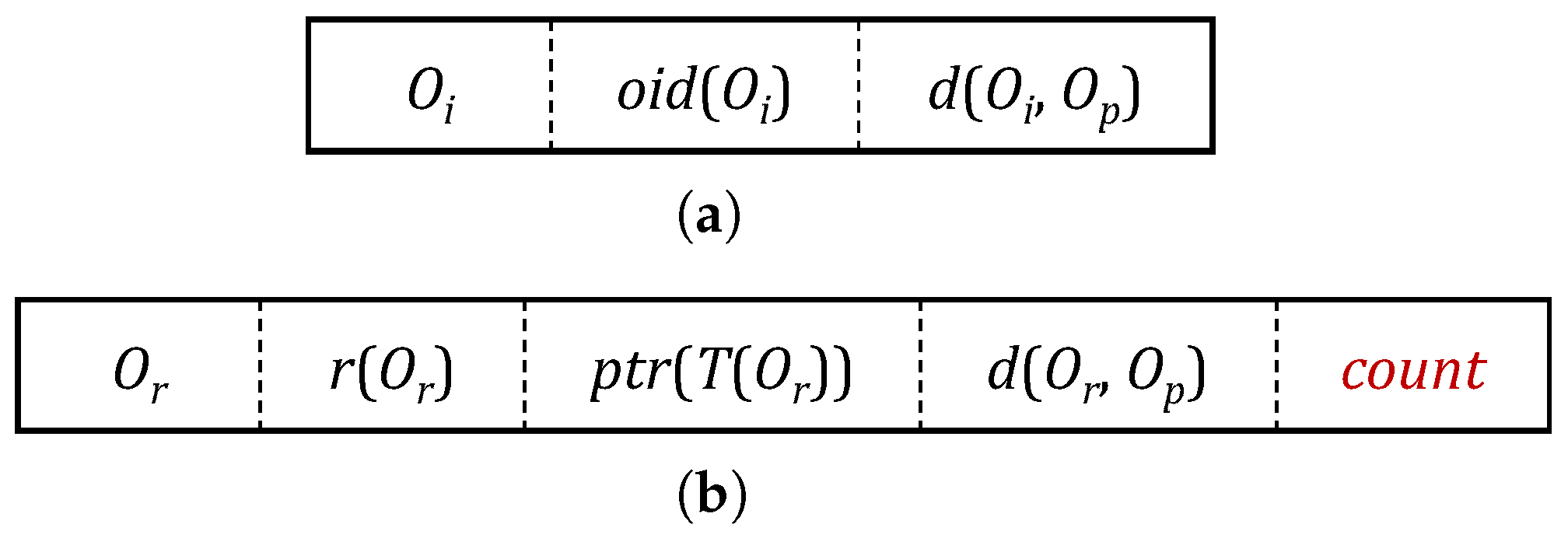
Figure 1 shows the node entry structures of the M-tree, and the description for each attribute is summarized in

Table 2. Attributes of a leaf node entry (Figure 1a).

Attribute	Description
$O_i$	an object
$oid\left(O_i\right)$	ID of $O_i$
$d(O_i,O_p)$	distance between $O_i$ and parent object $O_p$

and

Table 3. Attributes of a non-leaf node entry (Figure 1b).

Attribute	Description
$O_r$	routing object, i.e., parent object of n
$r\left(O_r\right)$	radius of spherical region of n
$ptr\left(T\left(O_r\right)\right)$	pointer to the subtree $T\left(O_r\right)$ rooted by n
$d(O_r,O_p)$	distance between $O_r$ and $O_p$ (parent node of N)
$count$	number of objects in the subtree $T\left(O_r\right)$

. The minimum bounding region containing all the objects in an M-tree leaf node L is represented as a sphere. In Table 2, the parent object $O_p$ is the central object that represents all the objects $O_i$ in the leaf node L. The entry structure of the M-tree leaf node used in our algorithm is the same as before. The minimum bounding region containing all the objects in an M-tree non-leaf node N is also represented as a sphere. In Table 3, n is the subnode of N corresponding to an entry e in N, and $O_p$ is the parent object of N. The region of node n is represented as a sphere centered by the routing object $O_r$ (i.e., the parent object of node n) with a radius of $r\left(O_r\right)$. The attribute count is newly added in our algorithm. If the node n pointed to by the pointer $ptr\left(T\left(O_r\right)\right)$ in an entry e is a leaf node, the value of $e.count$ is the number of all objects in the node n. If the node n pointed to by $e.ptr\left(T\left(O_r\right)\right)$ is a non-leaf node, the value of $e.count$ is set as $e.count=\sum e^{\prime }.count$ for all entries $e^{\prime }$ in node n. Thus, the count value for an entry e is the number of all objects contained in the subtree $T\left(O_r\right)$ rooted by the node n.

Algorithm 1 shows the AFANN-PHL algorithm. This algorithm has almost the same structure as the exact FANN-PHL [12]; the approximation task is added in line 14. In line 1 of Algorithm 1, ${\widehat{p}}^{*}$ is the current candidate FANN object, and H is the priority queue that includes the M-tree non-leaf entries e and is sorted in the ascending order of $e.g_{\varphi }$ values. In line 5, $e.n$ is the subnode corresponding to e, i.e., the root node of the subtree pointed to by the pointer $e.ptr\left(T\left(O_r\right)\right)$. In line 7, the FANN distance $e^{\prime }.g_{\varphi }$ of an entry $e^{\prime }$ is defined as follows [12]:

$$\begin{array}{c}\hfill e^{\prime }.g_{\varphi }=\underset{Q_{\varphi }\subseteq Q}{min}\left\{\mathcal{G}\{D(e^{\prime },q_i),q_i\in Q_{\varphi }\}\right\},\end{array}$$

(4)

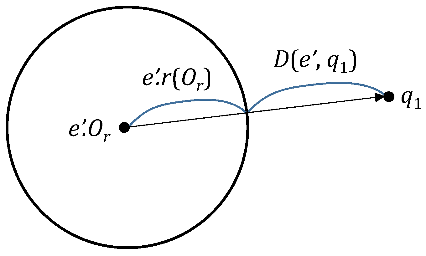
where $D(e^{\prime },q_i)$ is the distance between the spherical region for a node $e^{\prime }.n$ and a query object $q_i$; it is defined as $D(e^{\prime },q_i)=max\{D(e^{\prime }.O_r,q_i)-e^{\prime }.r\left(O_r\right),0\}$ (refer to Figure 2) [12].

Algorithm 1 AFANN-PHL Algorithm.

Require: $\mathcal{R},P,Q,\varphi ,\mathcal{G},T$ Ensure: $p^{*},Q_{\varphi }^{*},g(p^{*},Q_{\varphi }^{*})$   1: ${\widehat{p}}^{*}.g_{\varphi }\leftarrow \infty ,H\leftarrow ⌀$   2: $H.push\left(e\right)$ for all entries e in $T.root$   3: while $H\ne ⌀$ do   4:     $e\leftarrow H.pop\left(\right)$   5:     if $e.n$ is a non-leaf node then   6:         for each entry $e^{\prime }$ in $e.n$ do   7:            if $e^{\prime }.g_{\varphi }\le {\widehat{p}}^{*}.g_{\varphi }$ then $H.push\left(e^{\prime }\right)$ end if   8:         end for   9:     else 10:         for each object p in $e.n$ such that $p\in P$ do 11:            if $p.g_{\varphi }\le {\widehat{p}}^{*}.g_{\varphi }$ then ${\widehat{p}}^{*}\leftarrow p$ end if 12:         end for 13:     end if 14:     Invoke Algorithm 2 /* Perform approximation */ 15: end while 16: Return ${\widehat{p}}^{*}$

We first describe the case that the number of FANN objects k is 1, and the natural generalization for $k\ge 1$ is described later in this section. The approximate FANN object $p_{ϵ}^{*}$ returned by the AFANN-PHL algorithm for a given $ϵ$ (≥ 1) should satisfy the following condition for the exact FANN object $p^{*}$:

$$\begin{array}{c}\hfill p_{ϵ}^{*}.g_{\varphi }\le ϵ·p^{*}.g_{\varphi }.\end{array}$$

(5)

For $ϵ=1$, the AFANN-PHL returns the same result as the exact FANN-PHL. For $ϵ>1$, when the AFANN-PHL finds the object $p_{ϵ}^{*}$ that satisfies Equation (5) in line 14 of Algorithm 1, it returns the object and terminates right away. Therefore, since the algorithm terminates early even before the exact FANN object $p^{*}$ is found, it has the advantage of improving search performance. There is a tradeoff between the search performance and the accuracy of the approximate FANN object $p_{ϵ}^{*}$; it can be adjusted as needed by changing $ϵ$ appropriately. In Section 4, as the experimental result using real road network datasets, we show that the approximate FANN object $p_{ϵ}^{*}$ is very close to the exact FANN object $p^{*}$ even with a high value of $ϵ$.

In line 14 of Algorithm 1, the AFANN-PHL algorithm carries out the approximation task as described in Algorithm 2. In lines 1 and 2 of Algorithm 2, $H_{ϵ}$ is the priority queue created separately from H; a tuple $[{\widehat{p}}^{*},{\widehat{p}}^{*}.g_{\varphi },1]$ for the current candidate FANN object ${\widehat{p}}^{*}$ and a tuple $[e,e.g_{\varphi },e.count]$ for each entry e in H are inserted in $H_{ϵ}$. All the tuples in $H_{ϵ}$ are sorted in the ascending order of the second attribute values. In line 4, the tuple $t_a$ that satisfies the following Equation (6) is extracted:

$$\begin{array}{c}\hfill a=\underset{0\le j<|H_{ϵ}|}{min}\left\{j\left|\sum _{0\le i\le j}{t}_i.count\ge 1\right.\right\},\end{array}$$

(6)

where $t_i.count$ is the third attribute of a tuple $t_i$. If a tuple that satisfies Equation (6) does not exist, $t_a.g_{\varphi }$ is set as $t_a.g_{\varphi }=\infty$. If the condition in line 5 is satisfied for the tuple $t_a$, the algorithm returns the current candidate FANN object ${\widehat{p}}^{*}$ and terminates. Here, $t_a.g_{\varphi }$ is the second attribute of the tuple $t_a$.

Algorithm 2 Approximation by AFANN-PHL.

1: $H_{ϵ}.push\left([{\widehat{p}}^{*},{\widehat{p}}^{*}.g_{\varphi },1]\right)$ for current candidate FANN object ${\widehat{p}}^{*}$ 2: $H_{ϵ}.push\left([e,e.g_{\varphi },e.count]\right)$ for each entry e in H 3: Sort $H_{ϵ}$ in the ascending order of second attribute values 4: Find the tuple $t_a$ satisfying Equation (6) 5: if ${\widehat{p}}^{*}.g_{\varphi }\le ϵ·t_a.g_{\varphi }$ then return ${\widehat{p}}^{*}$ end if

The generalization of the AFANN-PHL algorithm for $k\ge 1$ is straightforward as follows. First, an array $K^{ϵ}$ is allocated to store the k approximate FANN objects, and Equation (5) is modified as the following:

$$\begin{array}{c}\hfill K_{k-1}^{ϵ}.g_{\varphi }\le ϵ·K_{k-1}.g_{\varphi },\end{array}$$

(7)

where $K_{k-1}$ is the exact k-th FANN object. The array $K^{ϵ}$ is always sorted in the ascending order of the values of $K_i^{ϵ}.g_{\varphi }(0\le i<k)$. In line 1 of Algorithm 2, a tuple $[K_i^{ϵ},K_i^{ϵ}.g_{\varphi },1]$ for each approximate candidate FANN object $K_i^{ϵ}$ is inserted, and in line 4, the tuple $t_a$ that satisfies the following Equation (8) is extracted:

$$\begin{array}{c}\hfill a=\underset{0\le j<|H_{ϵ}|}{min}\left\{j\left|\sum _{0\le i\le j}{t}_i.count\ge k\right.\right\}.\end{array}$$

(8)

The condition in the if statement in line 5 is modified to $K_{k-1}^{ϵ}.g_{\varphi }\le ϵ·t_a.g_{\varphi }$. The following Lemma 1 shows the correctness of the AFANN-PHL algorithm for the general case of $k\ge 1$, i.e., the returned approximate FANN objects satisfy Equation (7).

Lemma 1.

The approximate FANN object $K_{k-1}^{ϵ}$ returned by the AFANN-PHL algorithm satisfies Equation (7).

Proof. 

For each tuple $[e,e.g_{\varphi },e.count]$ in $H_{ϵ}$, any object p contained in the spherical region of the entry e satisfies $p.g_{\varphi }\ge e.g_{\varphi }$ [12]. For each tuple $[K_i^{ϵ},K_i^{ϵ}.g_{\varphi },1](0\le i<k)$ in $H_{ϵ}$, we associate a spherical region centered by the approximate FANN object $K_i^{ϵ}$ with a radius of 0. Since there are k or more objects in the spherical regions for the tuples $t_0,\dots ,t_a$ that satisfy Equation (8), it holds that $t_a.g_{\varphi }\le K_{k-1}.g_{\varphi }$, where $t_a.g_{\varphi }$ is the second attribute value of the tuple $t_a$, and $K_{k-1}$, is the exact k-th FANN object. If not, i.e., if it holds that $t_a.g_{\varphi }>K_{k-1}.g_{\varphi }$, all the objects p in the region for the tuple $t_a$ satisfy $p.g_{\varphi }>K_{k-1}.g_{\varphi }$. Moreover, since the tuples in $H_{ϵ}$ are sorted in the ascending order of the second attribute values, all the remaining tuples $t_i(i>a)$ satisfy $t_i.g_{\varphi }>K_{k-1}.g_{\varphi }$, and thus all the objects p in the region for $t_i$ satisfy $p.g_{\varphi }>K_{k-1}.g_{\varphi }$. That is, in the regions for the tuples $t_a,\dots ,t_{|H_{ϵ}|-1}$ in $H_{ϵ}$, we cannot find any FANN object. However, since there exist less than k objects in the regions for the tuples $t_0,\dots ,t_{a-1}$, there cannot exist k FANN objects, which is a contradiction. Therefore, it holds that $t_a.g_{\varphi }\le K_{k-1}.g_{\varphi }$. If the condition $K_{k-1}^{ϵ}.g_{\varphi }\le ϵ·t_a.g_{\varphi }$ is satisfied in line 5 of Algorithm 2, since it holds that $ϵ·t_a.g_{\varphi }\le ϵ·K_{k-1}.g_{\varphi }$, the AFANN-PHL algorithm satisfies $K_{k-1}^{ϵ}.g_{\varphi }\le ϵ·K_{k-1}.g_{\varphi }$ (Equation (7)). □

Our algorithm has the worst-case complexity for $ϵ=1.0$ since it cannot terminate early, and the complexity is the same as that of the exact FANN algorithm. The exact FANN algorithm has the worst-case complexity when the number and distribution of query objects are set so that the algorithm should access all leaf nodes in the M-tree. In this case, the shortest-path distances from all data objects $p(\in P)$ to all query objects $q_i(\in Q)$ should be calculated. Thus, the worst-case complexity of our algorithm is $O\left(\right|P\left|\right|Q\left|C\right)$, where C is the cost of the shortest-path distance calculation. However, the practical search cost is usually much lower than the worst-case complexity.

4. Experimental Evaluation

In this section, we carry out a series of experiments to compare the search performance of the existing exact FANN-PHL algorithm [12] and our AFANN-PHL algorithm and to verify the search accuracy of our algorithm for various approximation ratios $ϵ$. In our experiments, the performance of our algorithm is compared only with the FANN-PHL algorithm [12] since it is the state-of-the-art exact FANN search algorithm. The platform for the experiments is a workstation equipped with an AMD 3970X CPU, 128GB memory, and a 1.2TB SSD. Both FANN-PHL and AFANN-PHL algorithms were implemented in C/C++. In our experiments, to quickly calculate the shortest-path distance D between two objects (vertices), we used the C/C++ source code written by the original author of the PHL algorithm (http://github.com/kawatea/pruned-highway-labeling (accessed on 1 July 2023)).

The datasets in our experiments are the real-world road network datasets of five regions in the USA, which have also been used in the 9th DIMACS Implementation Challenge—Shortest Paths (http://www.diag.uniroma1.it/challenge9/download.shtml (accessed on 1 July 2023)) and in various previous studies [2,11,12].

Table 4. Road network datasets.

Acronym	Name	Vertices	Edges
NY	New York City	264,346	733,846
COL	Colorado	435,666	1,057,066
NW	Northwest USA	1,207,945	2,840,208
LKS	Great Lakes	2,758,119	6,885,658
W	Western USA	6,262,104	15,248,146

summarizes the experimental datasets. A road network dataset is represented as a graph composed of a set of vertices and a set of undirected edges. Each vertex represents a single object in a road network, and each edge represents a single road segment directly connecting two neighboring vertices. Since the datasets contain noises such as self-loop edges for a vertex and unconnected graph segments [2,11,12], we carried out preprocessing to remove the noises.

Table 5. Experiment parameters.

Parameter	Description	Values (Default Value)
$\mathcal{R}$	road network dataset	NY, COL, NW, LKS, W (NW)
M	size of Q, i.e., $\left|Q\right|$	64, 128, 256, 512, 1024 (256)
k	number of nearest neighbors	1, 5, 10, 15, 20 (1)
$\varphi$	flexibility factor	0.1, 0.3, 0.5, 0.8, 1.0 (0.5)
C	coverage ratio of Q	0.01, 0.05, 0.10, 0.15, 0.20 (0.10)
$ϵ$	approximation ratio	1.0, 2.0, 3.0, 4.0, 5.0 (5.0)

summarizes the parameters considered in our experiments; the values in parentheses indicate default values.

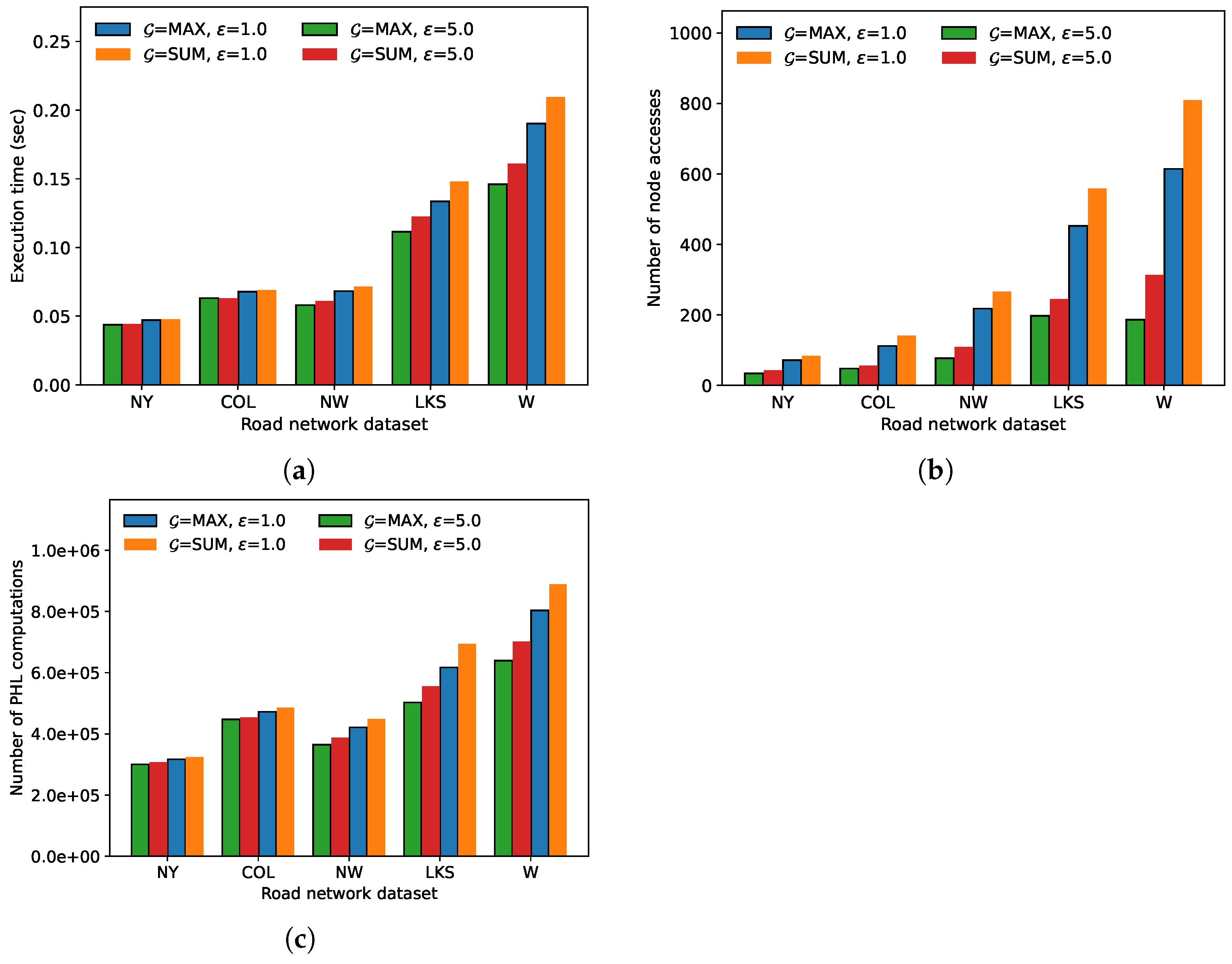
In the first experiment, we compared the execution time, the number of node accesses, and the number of distance D calculations needed for the FANN search for each road network dataset in Table 4. Here, all the other parameter values were set to their default values indicated in Table 5. For each parameter combination, we averaged the results obtained using an arbitrary 1000 query sets Q. Figure 3 demonstrates the results of the first experiment. The execution time, the number of node accesses, and the number of distance calculations show similar trends for both algorithms. As the number of objects in a road network increases, the number of index nodes within a query region of the same size increases. Thus, the number of distance calculations to the objects in the index nodes also increases, thereby making the execution time of the algorithms increase. In the first experiment, the AFANN-PHL algorithm always showed a higher performance than the exact algorithm; for the W dataset, the performance improved by up to 30.3% for $\mathcal{G}=$ max.

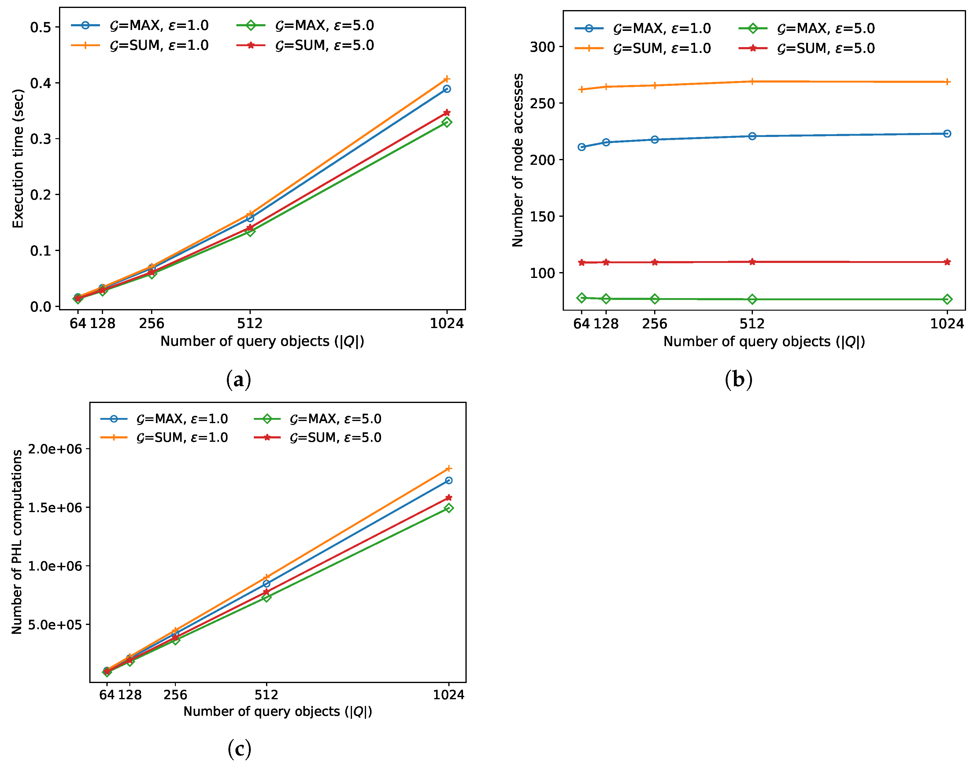
In the second experiment, we compared the FANN search performance for various query sizes M. As demonstrated in Figure 4, the execution time and the number of distance calculations increases almost linearly as M increases for both algorithms. This is because both algorithms need to calculate the exact distances D to M query objects $q_i$ to find both ${\widehat{p}}^{*}.g_{\varphi }$ and $e^{\prime }.g_{\varphi }$ [12]. Meanwhile, the number of node accesses has not changed much as M increases for both algorithms. This is because, if the regions containing the query objects are similar, both ${\widehat{p}}^{*}.g_{\varphi }$ and $e^{\prime }.g_{\varphi }$ remain similar even though M increases [12]. In this experiment, the approximate algorithm always outperformed the exact algorithm; the performance improved by up to 18.7% when $M=64$ and $\mathcal{G}=$ sum.

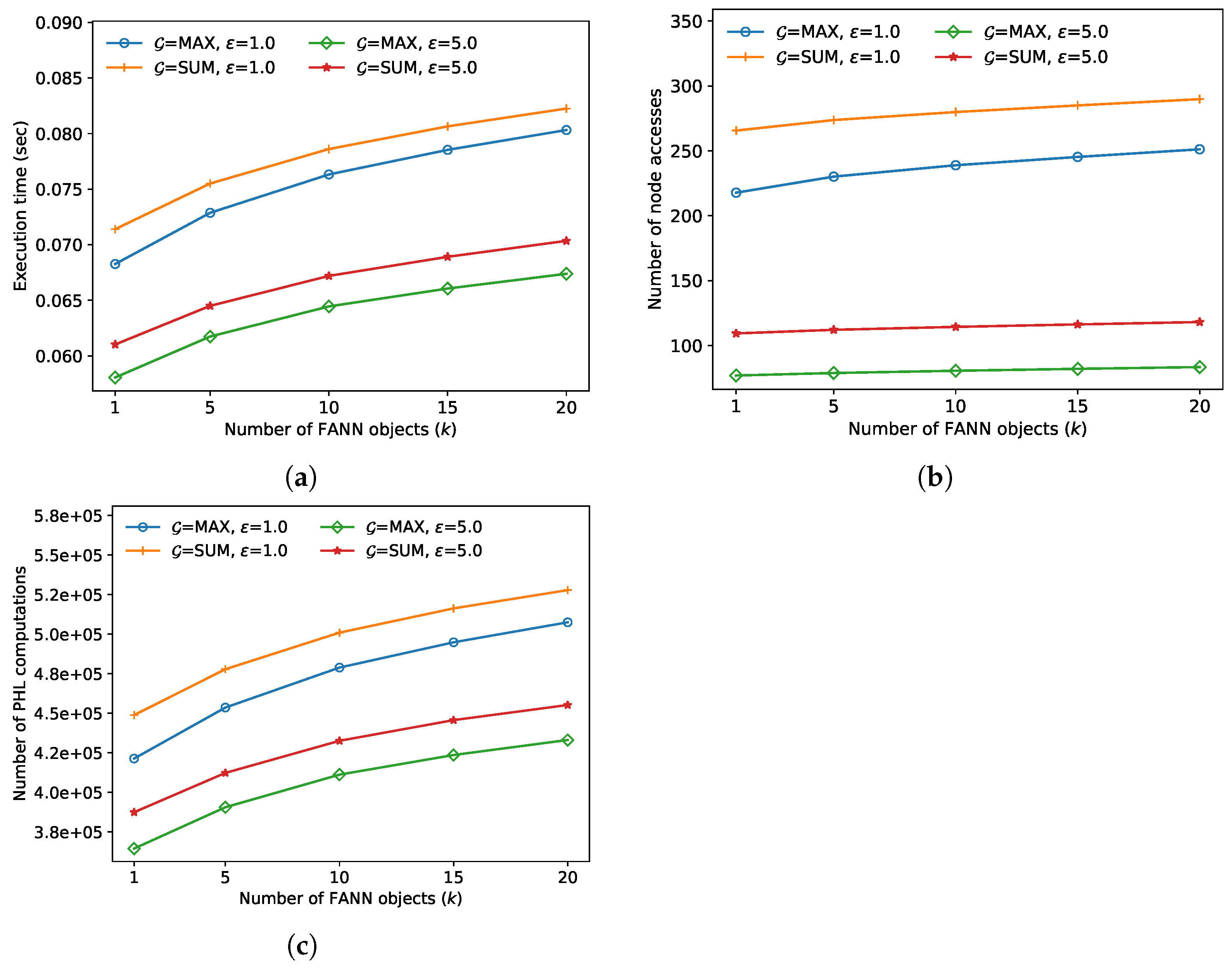
In the third experiment, we compared the FANN search performance for various numbers of nearest neighbors k, and the results are demonstrated in Figure 5. For both algorithms, in lines 7 and 11 of Algorithm 1, the pruning bounds become larger as k increases. Thus, more index nodes are accessed, and more distance calculations to the objects in the index nodes are performed, thereby increasing the execution time of both algorithms. In this experiment, the approximate algorithm always outperformed the exact algorithm; the performance improved by up to 19.2% when $k=20$ and $\mathcal{G}=$ max.

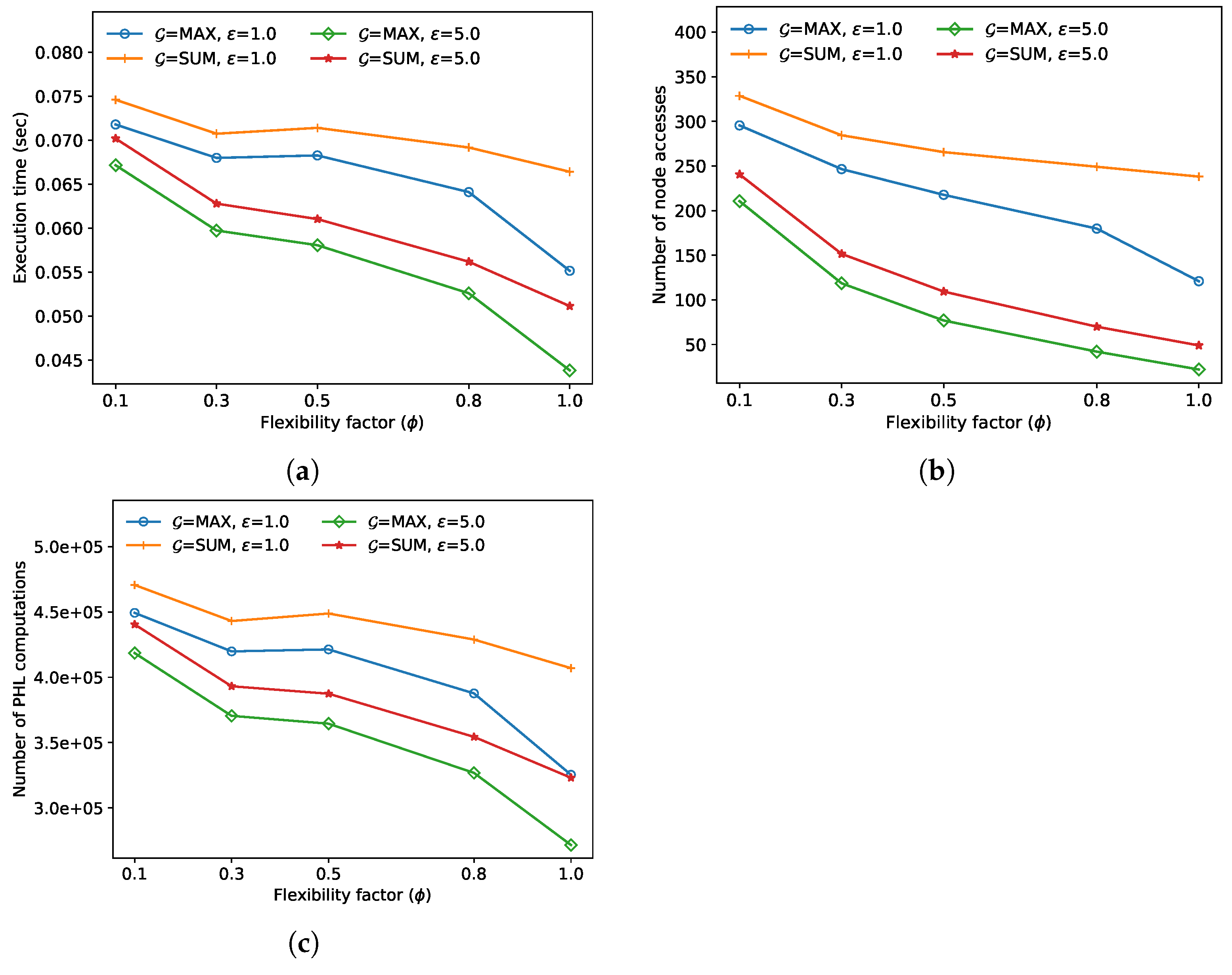
In the fourth experiment, we compared the FANN search performance for various flexibility factors $\varphi$. In Figure 6, as $\varphi$ increases, the execution time, the number of node accesses, and the number of distance calculations tend to decrease for both algorithms. This is because, as $\varphi$ increases in line 7 of Algorithm 1, ${\widehat{p}}^{*}.g_{\varphi }$ increases more rapidly than $e^{\prime }.g_{\varphi }$, and thus the number of entries $e^{\prime }$ added in the priority queue H decreases. In this experiment, the approximate algorithm always outperformed the exact algorithm; the performance improved by up to 29.9% when $\varphi =1.0$ and $\mathcal{G}=$ sum.

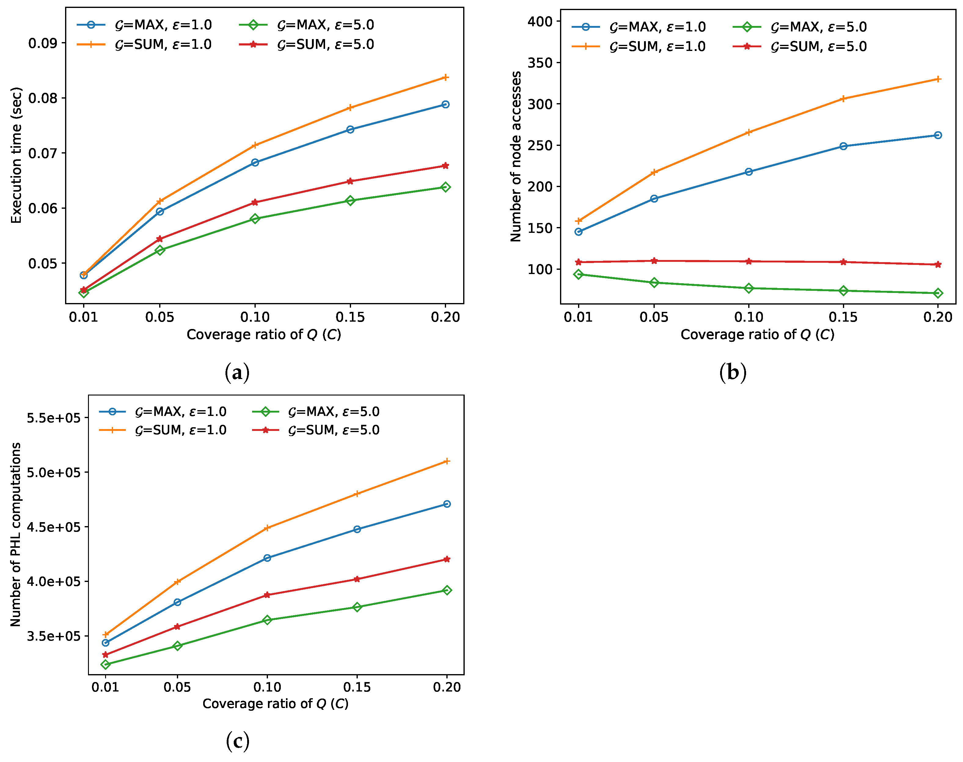
In the fifth experiment, we compared the FANN search performance for various coverage ratios $C(0<C\le 1)$ of query sets Q, where C is defined as (the minimum region covered by all the query objects in Q) divided by (the region covered by the whole road network). The results of this experiment are demonstrated in Figure 7. As C increases, the execution time, the number of node accesses, and the number of distance calculations increase generally. The number of node accesses of the approximate algorithm decreases as C increases. That is because the approximate algorithm terminates early very often as $t_a.g_{\varphi }$ increases in line 5 of Algorithm 2. In this experiment, the approximate algorithm always outperformed the exact algorithm; the performance improved by up to 23.7% when $C=0.2$ and $\mathcal{G}=$ sum.

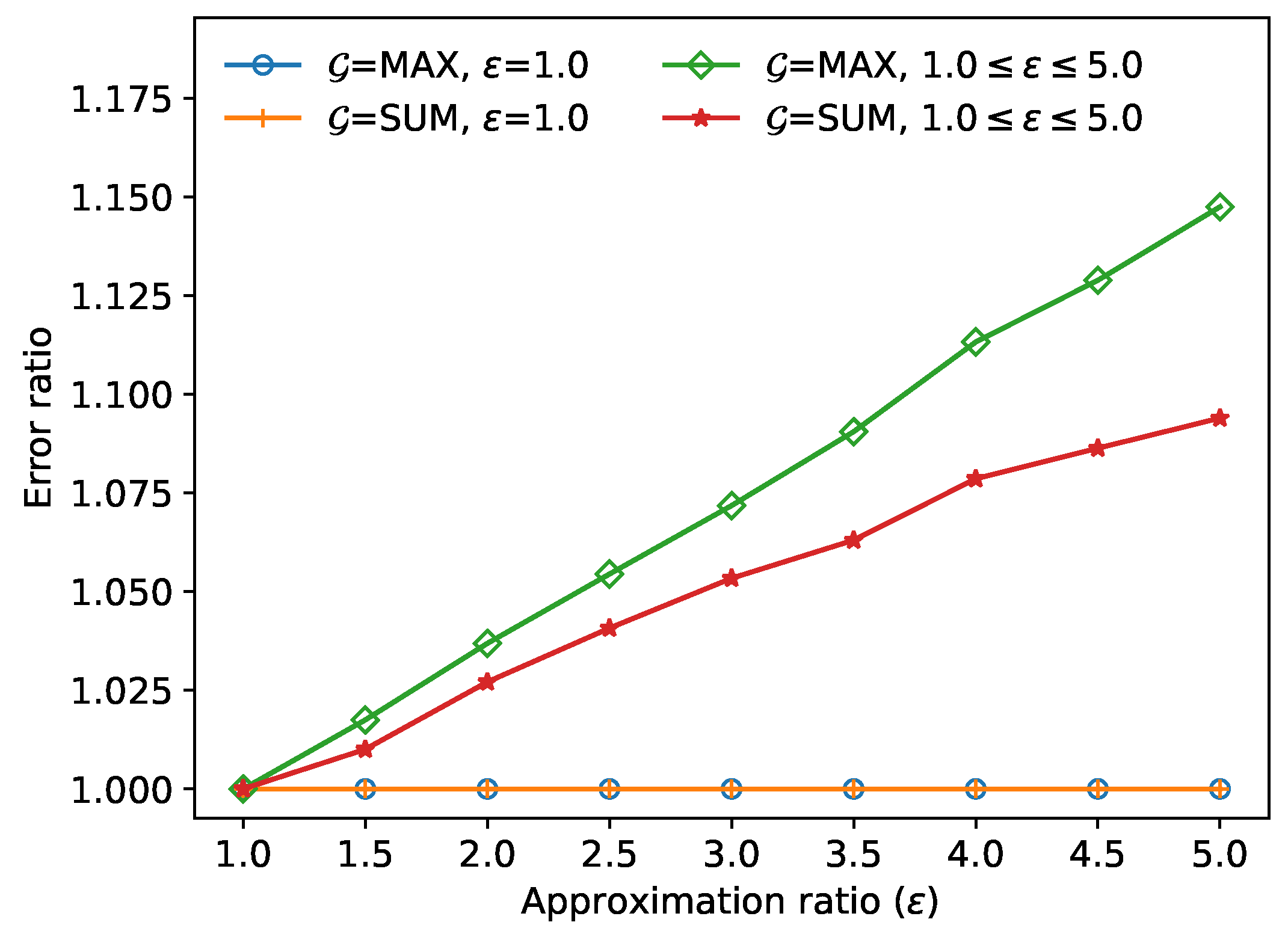
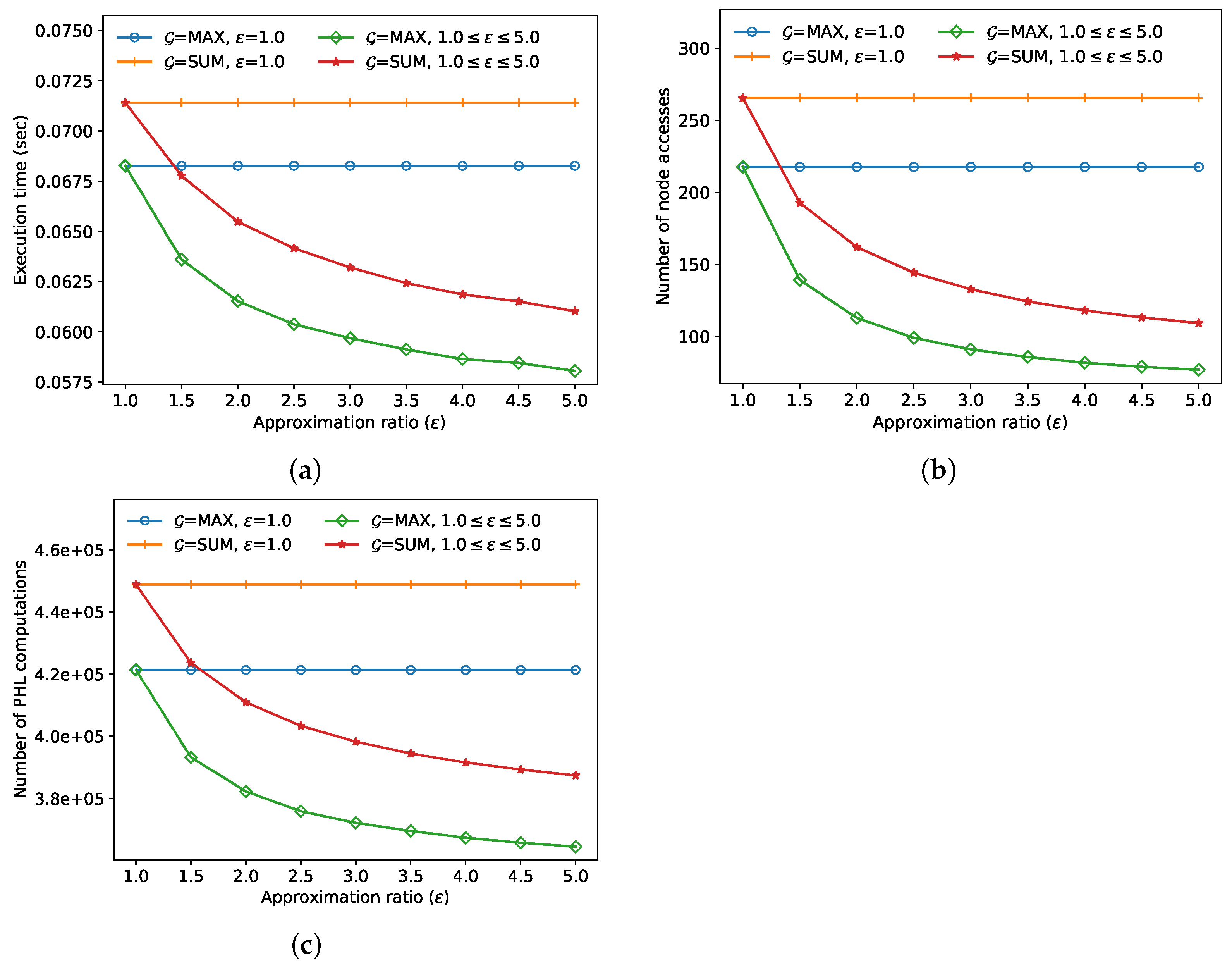
In the final experiment, we compared the FANN search performance and accuracy for various approximation ratios $ϵ$. In Figure 8, the execution time, the number of node accesses, and the number of distance calculations of the AFANN-PHL algorithm decrease as $ϵ$ increases, as expected. In this experiment, the approximate algorithm always outperformed the exact algorithm; the performance improved by up to 17.6% when $ϵ=5.0$ and $\mathcal{G}=$ max. Figure 9 demonstrates the error ratio $\rho =p_{ϵ}^{*}.g_{\varphi }/p^{*}.g_{\varphi }$ (i.e., the left-hand side of Equation (3)) for the FANN objects $p_{ϵ}^{*}$ and $p^{*}$ obtained in the approximate and the exact FANN algorithms, respectively. The largest error ratio was $\rho =1.147$ when $ϵ=5.0$ and $\mathcal{G}=$ max. This value $\rho$ is much smaller than the given approximation ratio $ϵ$; i.e., the approximate FANN object $p_{ϵ}^{*}$ is very close to the exact FANN object $p^{*}$.

5. Conclusions

In this paper, we proposed an $ϵ$-approximate k-FANN search algorithm for arbitrary approximation ratios $ϵ$ (≥1) in road networks $(k\ge 1)$. In general, $ϵ$-approximate algorithms are expected to give an improved search performance at the cost of allowing an error ratio of up to the given $ϵ$. Since the optimal value of $ϵ$ highly depends on applications and cases, the approximation algorithm for an arbitrary $ϵ$ is essential. We proved that the error ratios of the approximate FANN objects returned by our algorithm do not exceed the given $ϵ$. To the best of our knowledge, our algorithm is the first $ϵ$-approximate k-FANN search algorithm in road networks for arbitrary ratios $ϵ$. We performed a series of experiments using various real-world road network datasets to demonstrate that our approximation algorithm always outperformed the state-of-the-art exact FANN search algorithm named FANN-PHL [12] for any parameter combinations. We had a better search performance with a higher $ϵ$ value. Furthermore, we also demonstrated that the error ratios of the approximate FANN objects returned by our algorithm were much lower than the given $ϵ$ values; i.e., we could find the approximate FANN objects that were very close to the exact FANN objects even with a high approximation ratio $ϵ$. Therefore, we expect that our algorithm could be widely adopted in many real-world location-based applications.