2. System Model
2.1. System Description
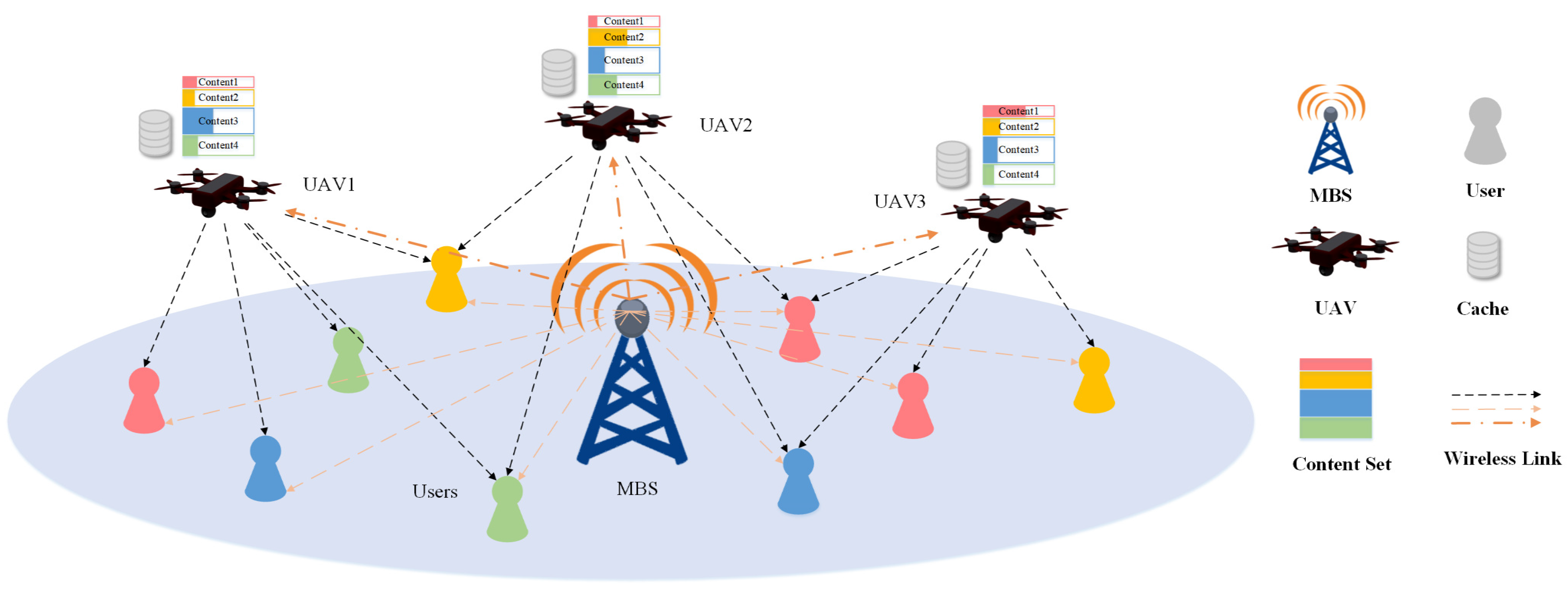
As shown in
Figure 1, we consider the downlink of a distributed cache network consisting of one MBS, UAVs and ground users. The set of UAVs is denoted by
, and the set of users is denoted by
. Assume that the number of antennas for each UAV is the same, and the number is
. Consider that there are
K popular content, denoted by set
.
Compared with MBS, UAVs are usually closer to users, so they provide higher transmission rates for related users. To simplify the discussion, it is assumed that the service rate of an MBS for each user is the same. The service rate of an MBS is set as a constant, which is lower than the average of UAVs.
2.2. UAVs and User Distribution Model
Without loss of generality, we assume all UAVs always hover at a constant height H. During the interested time slot, the positions of users are considered to be quasistatic, while all the horizontal positions of UAVs can be changed over time.
We denote the UAV as , and the user as , . The position vectors of and are denoted by and , respectively. For convenience of the subsequent formula expressions, we denote the position vector of the antenna of as , , and if is required for the content, denote the position of as , where .
We assume that each UAV serves several nearest users and each user could be served by several UAVs. For simplicity, the user association is considered to be fixed, which means the connection between UAVs and users would be unchanged during the interested time. The connection relationship between
and
is denoted by
.
represents that a connection exists, and
represents that a connection does not exist. That is,
The set of users served by is denoted as , , and .
2.3. Content Request, Caching and Fetching
In the considered system, each user randomly requests content following a certain probability distribution. We denote the probability of content
k being requested as
,
and
. For convenience, it is assumed that the content has been sorted by popularity, which means that content
k is the
most popular content of all content. Content popularity is modeled using a Zipf distribution, and the probabilities of popular content being requested by a user can be described as
, and the probability of requesting the
most popular content is
In (2), is called the Zipf parameter, and . Zipf distribution indicates the popularity of the content, and affects the differences in content popularity. The smaller the parameter is, the smaller the popularity differences among content will be, and the converse is also true. In extreme cases, if , all content will have the same probability of being requested, or if , the probability of content being requested will be in an inverse ratio to the ranking of the content.
The MBS is considered to be available for all users in the system and cached all contents. Differently, due to the limited power and capacity, each UAV can only connect some of the users and cache some of the content. Every UAV could choose to cache a complete content or just a part of it. The size of the content is denoted by , and proportion of the content cached in is denoted by , , , . UAVs are able to implement the caching strategy through the high-capacity backhaul link with the MBS, which means that is changeable and that limited storage of UAV could be reasonably allocated.
As for content fetching, UAVs and MBS cooperatively provide content for users. When the user initiates a data file request, the UAV serving the user only transmits the part of the file cached by the BTS, and the user reconstructs the file data from every connected UAV to obtain a complete file. If the requested file is not cached in the related UAVs, the missing file or part will be provided by MBS.
2.4. Signal, Channel and Noise Model
The number of antennas of each UAV is
; thus, the transmit signals could be denoted by
-dimension vectors. We denote the beamforming vector of the transmit signal
sent to
as
where
is a complex vector.
The channel coefficient between
and the
antenna of
is denoted by
, which consists of two parts: path loss and small-scale fading. We denote that
, where
reflects the pass loss, while
represents the small-scale fading.
is a function of
and
, described as
is considered to follow a Rician distribution. We adopt a Rician channel in our system model because a line of sight (LoS) signal usually exists in a UAV-assisted network. A Rician channel can be decomposed into a LoS propagation channel and a scattering channel, as shown in Equation (5).
where
and
represent the LoS component and NLoS component, respectively, and
usually follows a Rayleigh distribution.
is the parameter of the Rician distribution, which determines the proportion of LoS and NLoS in the channel. These parameters are considered to be constant during the interested time slot. Let
and
Then, we can denote the channel between and as , where ∘ is the operator of the Hadamard product. Here, is a constant complex vector, and is a complex vector variable. is a function of variable , so it is also denoted as .
It is assumed that MBS uses different frequency resources from UAVs, so there would be no interference between MBS and UAVs. Additive white gaussian noise (AWGN) and the interferences among UAVs are both considered. The signal to interference plus noise ratio (SINR) of the downlink transmission from
to
could be denoted as
where
represents the power of AWGN. The transfer data rate from
to
could be calculated using
Specially, we denote the downlink data rate between MBS and as . To simplify the discussion, is set as constant for , where the link details of MBS are not considered. Generally, we set as a lower value compared with because UAVs could usually achieve higher data rate by getting closer to users.
3. Problem Formulation and Solution
We minimize the average transmission latency of the network, which is related to locations, beamforming and caching strategies of UAVs. Specifically, the calculation of average latency is
where
R is the data rate, which is related to the beamforming weight
and path loss
, and
is mapped to UAV locations
. The system latency consists of two parts: MBS transmission latency and UAV transmission latency.
The related latency minimization problem is formulated as follows:
where
Here, inequality (10b) is the power constraint. The transmit power of UAV is limited, and we assume that the maximum power budget of every UAV is P. Equation constraint (10c) reflects the relationship between path loss and UAV location . Inequality (10d) is the capacity constraint of every UAV, ensuring the cached contents are not larger than the capacity . Inequality (10e) represents the content integrity constraint. For all popular content, the data transmitted by MBS should be able to be combined into complete content with the data transmitted by UAVs, as is shown in (10e). Furthermore, (10f) reflects the physical meaning of as the caching proportions.
As shown in (10a), caching variable , UAV location variable and beamforming variable in the objective function are coupled, which means that it would be quite difficult to solve the problem directly. In order to reduce the complexity of the solution, a step-by-step iterative optimization method is adopted. We fix one of the variables, solve the remaining variables and iteratively solve the original problem.
We fix the caching variable
first, and the proportion of the content
k cached in
is set as
. Then, the optimization problem becomes
Here, inequality (11c) is the relaxed version of the equality constraint (10c). Since the optimality always occurs at the equality, the relax of the constraint would not cause any loss of generality, and this treatment could reduce the complexity of the problem.
Due to the complex form of the denominator, the whole function is non-convex in (10a). We introduce variable and its constraint, so that the objective function (11a) is convex now. Note that the constraint of is also a relaxed version, and it is easy to prove that constraint (11d) turns into the tight constraint when the problem (11) obtains the optimal solution, which means that is equal to when the optimal problem is solved.
Problem (11) is still not a convex problem due to constraints (11c) and (11d) being neither concave nor convex. For (11c), we can make the left-hand side linearized via the first-order Taylor expansion, as shown in (12).
where
represents the Taylor expansion point.
We now consider transforming inequality (11d) into a convex constraint via DC method. The basic idea of DC method is, first, to transform the original problem into the difference of two convex functions, and, then, to apply an approximation method to eliminate the non-convexity.
For inequality (11d), we introduce a strongly convex function, which is added to and then taken away from the right-hand side of the original inequality, as shown in inequality (13). Inspired by [
21], we choose a quadratic form as the introduced strongly convex function. We write inequality (11d) as
In inequality (13),
is a positive constant we set. It is proved in [
21] that, if
is set to be positive and large enough, function
will have strong convexity. Although the form of
is non-convex and non-concave, the sum of
and the introduced function would be a convex function, as long as the convexity of the introduced function is strong enough. In this way, a form of difference between two convex functions is constructed. Let
then constraint (13) is changed into
Constraint (15) is in the form of the difference of two convex functions. To actually eliminate the non-convexity, we need to apply an approximation method, as it is noted earlier. The factor leading constraint (15) to be non-convex is because it is a convex function on the right-hand side of “≤”. We tighten constraint (15) by replacing with its lower-bound Taylor linearization. The first-order Taylor expansion for can change the original formula into a convex constraint. The gradient of is defined as .
As shown in Equation (8), the transmission rate
has a complicated form, which is mainly caused by the SINR part. There are a series of summations of variables, making the derivative of
hard to express. To deal with this, we bring out a method to convert the summations into matrix multiplications and subsequently derive the gradient for applying the linear approximation. We reconstruct the optimization variables by introducing a series of vectors and matrices. Let
As one of optimization variables in this problem, is a vector variable with dimensions, contains all beamforming weight information. The expression of SINR in matrix form can be constructed as follows:
Denote
,
,
, and then, let
Note that every
is a
-dimension square matrix and that
is a block diagonal matrix with
blocks. Specifically, the diagonal blocks of
are divided into
M groups, and each group contains
N blocks. Every diagonal block is a
matrix, so we can see that each
is a square matrix with
dimensions. Actually,
consists of a series of
and zero matrices. The
N blocks of a group are all nearly the same, except the
block of every group is a zero matrix. Furthermore, the
N blocks of the
group are all zero matrices. Except those above blocks, the blocks in the
group are set as
. The blocks of the
group roughly represent the channels between interference source
and
. For the downlink channel from
to
, the interference caused by signals sent from other UAVs to other users can be represented by
. Let
is almost the same as
; the only difference is the
block in the
group. To be specific, the
block of
is
instead of
. Then, we can give a concise form of the channel data rate as follows:
The partial difference of
for
can be calculated as
At this point, we have reconstructed the expression of , and it is much easier to seek the partial difference of in Equation (19), compared with Equation (8). The main idea behind this proposed reconstruction method is to specially design the variables as structured vectors and to construct the form of matrix multiplications according to the summations in the original expression. This method turned out to be effective in dealing with complicated summations, such as the interference among UAVs in this study.
Equation (19) is a concise form with respect to variable . To obtain the partial difference for , we need to construct a new form of . Let , , , . The dimension of vector is , and every is a -dimension square matrix.
We define
and
where
, as defined in (7). Every
is a vector with
dimensions, and
is a vector with
dimensions, which consists of
for all
. We use
as one of the optimization variables and seek the partial difference for it. Let
and
Note that the only difference between
and
is that
has one more summation term than
. Similar to (19), we can transform (8) into
The partial difference of
for
can be calculated as
The first-order Taylor expansion for
at
,
is denoted as
:
Until now, the optimization subproblem (11) has been converted as
Problem (30) is a convex optimization problem, and it is a transformation of problem (11), which corresponds to the optimization of UAV location and beamforming variables with caching variable fixed.
Then, we oppositely consider optimizing a caching variable with the UAV location and beamforming variables fixed. UAV caching optimization subproblem is formulated as
It is obvious that problem (31) is a linear programming problem.
Algorithm 1 outlines the DC-based method to solve (10).
| Algorithm 1: The DC-based joint optimization algorithm. |
Initiation: 1. Set user positions and connection relationship . 2. Set the iteration number , and initialize start values of , and . Calculate from and . Repeat: 3. Solve problem (30) to obtain the optimal solutions , . Calculate from and . 4. Solve problem (31) to obtain the optimal solution . 5. . 6. , , . convergence of the objective function in (30). 7. Output , and as the optimal solution. |
4. Simulation Results
In this section, Matlab-based simulations are presented, and we evaluate the performance of the proposed joint optimization algorithm through numerical results. In our simulations, we randomly distribute ground users in a square area, and the number of users is . We set the number of UAVs as , and the initial locations of the UAVs are roughly uniformly distributed. Specifically, we decided the connection relationships first, in which each user is served by two UAVs. The initial locations of UAVs are set as the average location of served users. We also set the UAV altitude as , the antenna number as , and the popular content amount as . As for channels, we set the , , and as a complex random number with an average modulus of 1 in Equation (5). Moreover, we define the ratio of total capacity of UAVs to the total size of popular content as the UAV capacity coefficient, denoted by , which represents the capacity-to-content ratio. Specifically, we decide the capacity limit of UAVs as in constraint (31b).
To show the effectiveness of the DC-based optimization algorithm, we present two benchmark algorithms, denoted by Algorithms 2 and 3, respectively. Algorithm 2 optimizes the beamforming and caching strategy with the UAV locations fixed, while Algorithm 3 optimizes the beamforming and UAV locations with cache fixed. These two benchmark algorithms are both variants of the proposed DC-based algorithm, and they are supposed to help evaluate the impact of different optimization variables in this model. Furthermore, we change the parameters in simulations to observe the performance changes in the algorithms.
The optimization problem of Algorithm 2 is shown in (32).
Algorithm 2 optimizes the beamforming and caching strategy iteratively, and the UAV locations are fixed as the average position of the connected users. In the case of Algorithm 2, the system is similar to a traditional cache network, with several small cellular base stations in it. To ensure the rigor of the conclusions, Algorithm 2 adopts the same DC-based method and reconstruction method as Algorithm 1, although the form is simplified because of the reduction in optimization variables.
Algorithm 3 is a variant with cache fixed, which jointly optimizes UAV location and beamforming. For reasonableness, we consider the cache occupied by each content being proportional to its size in Algorithm 3, where the proportion of every content cached in each UAV is . Compared with Algorithm 1, Algorithm 3 eliminates the step of cache iterative optimization, and the other steps are almost the same.
Compared with Algorithm 1, the benchmark Algorithm 2 indicates the impact of UAV location optimization, while Algorithm 3 reflects the effect of caching optimization. The two benchmark algorithms are outlined in Algorithms 2 and 3.
| Algorithm 2: The beamforming and caching iterative optimization algorithm. |
Initiation: 1. Set user positions and connection relationship . Set to the average of connected users’ positions. Calculate from and . 2. Set the iteration number , and initialize start values of and . Repeat: 3. Solve problem (32) to obtain the optimal solutions . 4. Solve problem (31) to obtain the optimal solution . 5. . 6. , . convergence of the objective function in (32). 7. Output and as the optimal solution. |
| Algorithm 3: The joint beamforming and location optimization algorithm. |
Initiation: 1. Set user positions and connection relationship . Set every elements of to . 2. Set the iteration number , and initialize start values of , . Calculate from and . Repeat: 3. Solve problem (30) to obtain the optimal solutions , . Calculate from and . 4. . 5. , . convergence of the objective function in (30). 6. Output and as the optimal solution. |
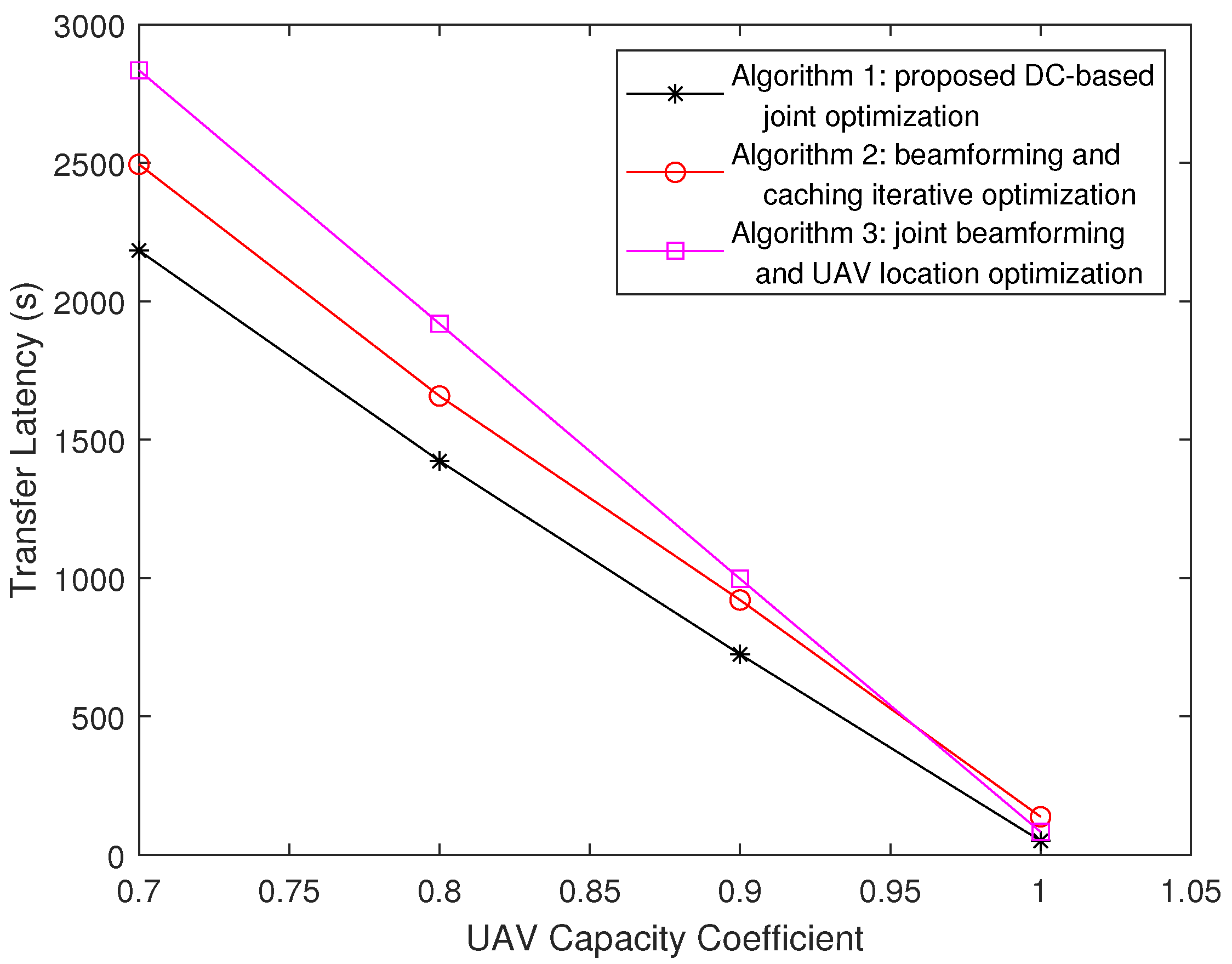
Firstly, we observe the impact of the UAV capacity coefficient
on the system latency. We set the Zipf parameter
. As it is shown in
Figure 2, the latency performance of the proposed algorithm is better than those of the two benchmark algorithms. The delay decreases with the increase in UAV coefficient, which means expanding the cache capacity of UAVs would achieve a higher network efficiency. And, note that the average transmission latency of Algorithm 3 gets closer and closer to that of proposed Algorithm 1, while
changes from 0.7 to 1. When
, the latency of Algorithm 3 is almost the same as that of Algorithm 1 because if
, which means UAVs obtain enough capacity to cache all the contents, users do not need to request content from MBS. In this case, the content placement in UAVs has little impact on the average transmission latency.
Then, in
Figure 3, we consider the impact of Zipf parameter
. The UAV capacity coefficient is set as
. We increase
from 0.3 to 1, and it is observed that the latency of Algorithm 1 is decreased. Predictably, the performance of Algorithm 2 is relatively poor compared with Algorithm 1, and the trend of its curve is consistent with that of Algorithm 1. Note that the performance of Algorithm 3 is much worse and that the trend of its curve is different from those of Algorithms 1 and 2. Via an analysis, the reason behind the difference is whether the caching strategy is optimized. Content placement is fixed in Algorithm 3, and the trend of its curve is related to the sizes of the files. The latency of Algorithm 3 is directly proportional to the expectation of the content size. If the size of content with a high popularity is relatively larger, the expectation of the content size will increase with the increase in the Zipf parameter; otherwise, the opposite happens. Especially, if all the contents are the same size, no matter how the request probability changes, the expectation of the content size will not change, and the curve mentioned above tends to be a horizontal straight line. In general, we can observe that the optimization of the caching strategy is more effective when the Zipf parameter is larger.
Furthermore, the impact of UAV altitude is considered. We vary the height of UAVs from 100 m to 500 m, and the latency performance is shown in
Figure 4. The curves of three algorithms are generally flat and very slowly ascending. We consider that all the interference between UAVs exists simultaneously in the system, and accordingly, the interference has a significant impact on the system latency. As the UAV height increases, the received signal weakens and the interference also decreases; as a result, the overall transmission delay remains almost stable. Note that the curves show a slight upward trend because the AWGN will not decrease as the height increase, which causes a decrease in SINR. The proposed Algorithm 1 performs better than the other two in different UAV height situations.
After a comparison and analysis, we found that the performance of Algorithm 2 is usually better than Algorithm 3, excluding the situation that the UAV capacity is extremely large. This indicates that the caching strategy plays a more important role than UAV locations in this system model. Moreover, the proposed DC-based algorithm performs better in situations where the Zipf parameter of content popularity is large or the UAV caching capacity is limited.

