
FURSformer: Semantic Segmentation Network for Remote Sensing Images with Fused Heterogeneous Features

Abstract
1. Introduction
2. Related Work
3. Methods and Motivation
3.1. Research Motivation
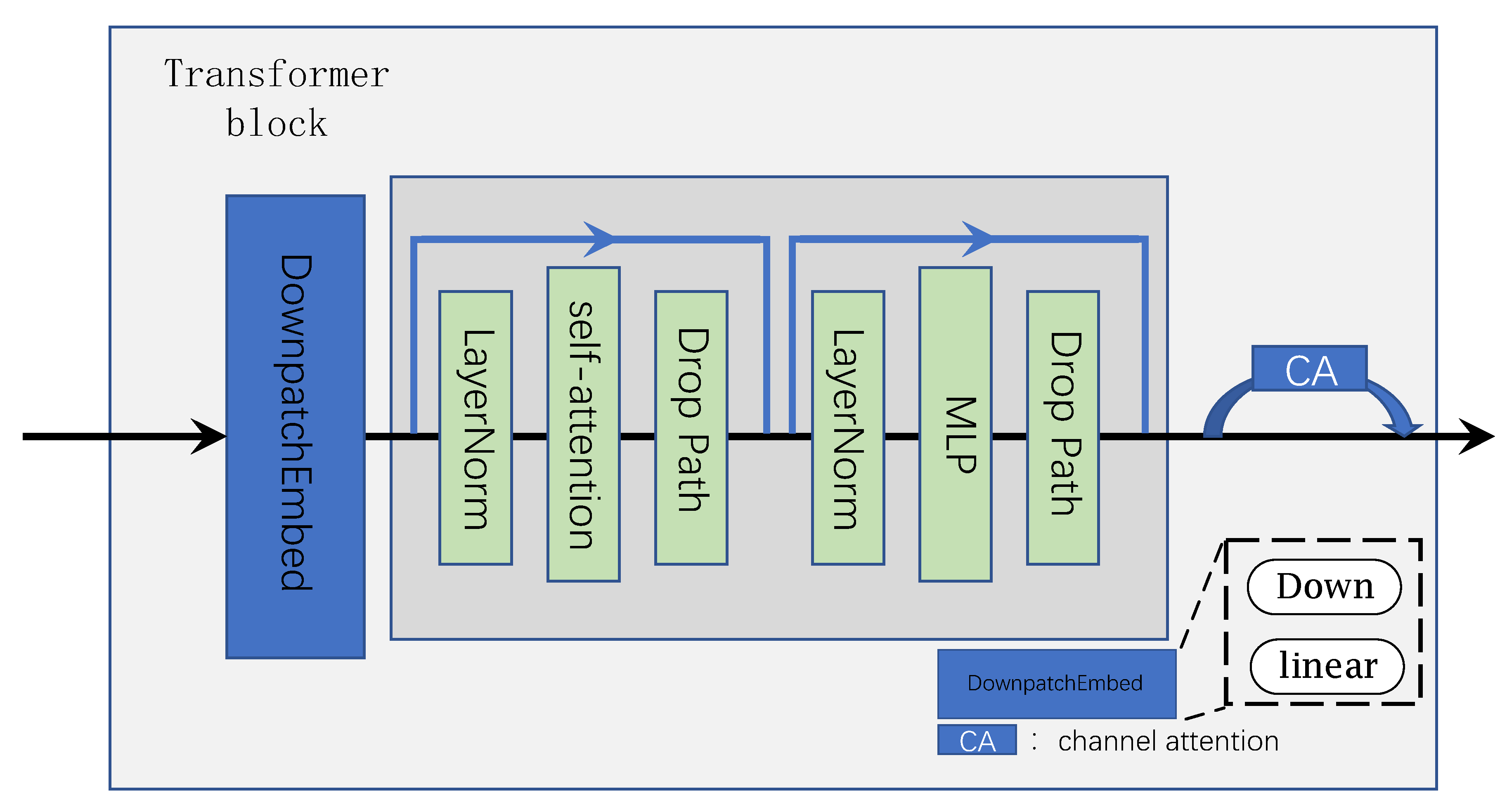
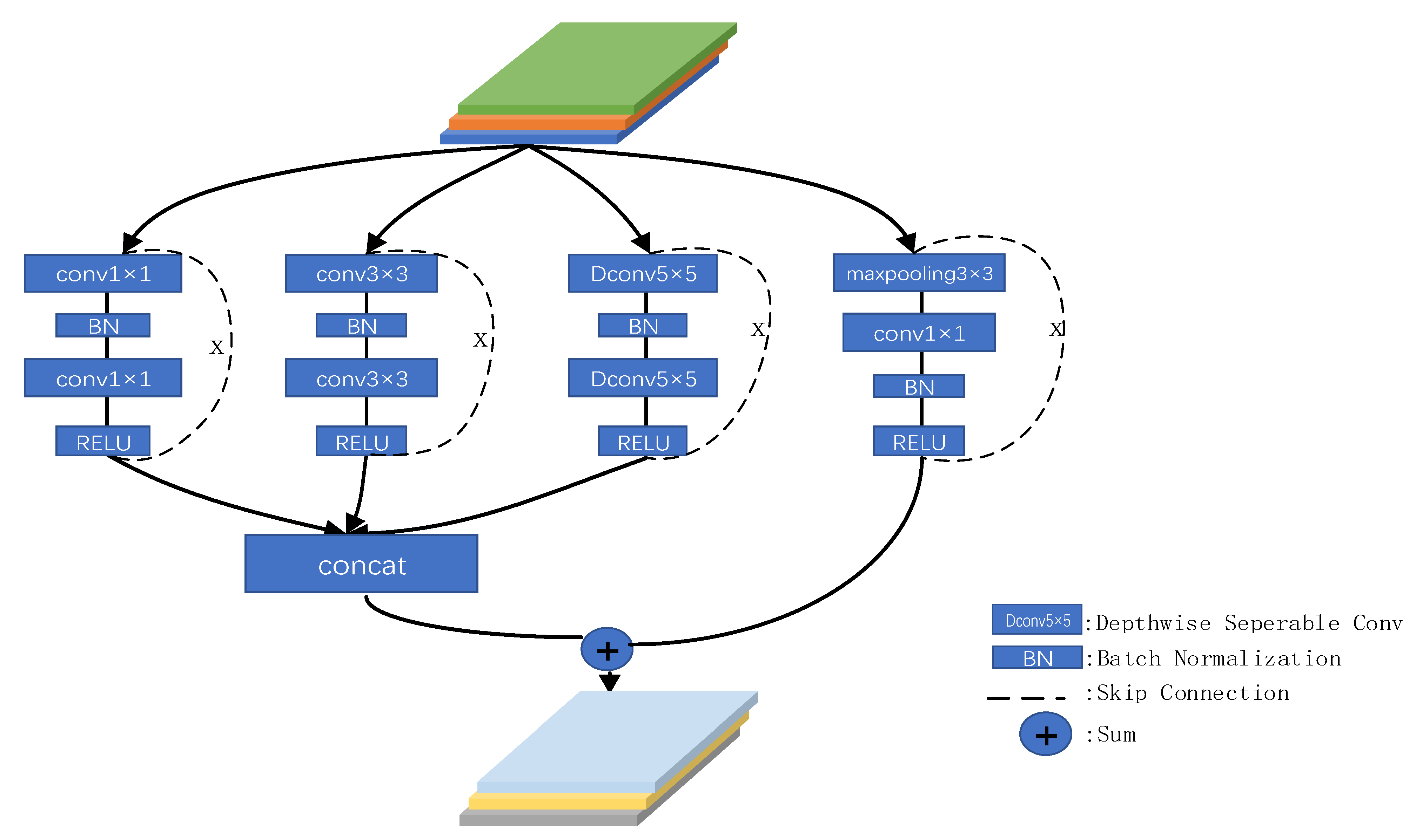
3.2. Transformer and CNN
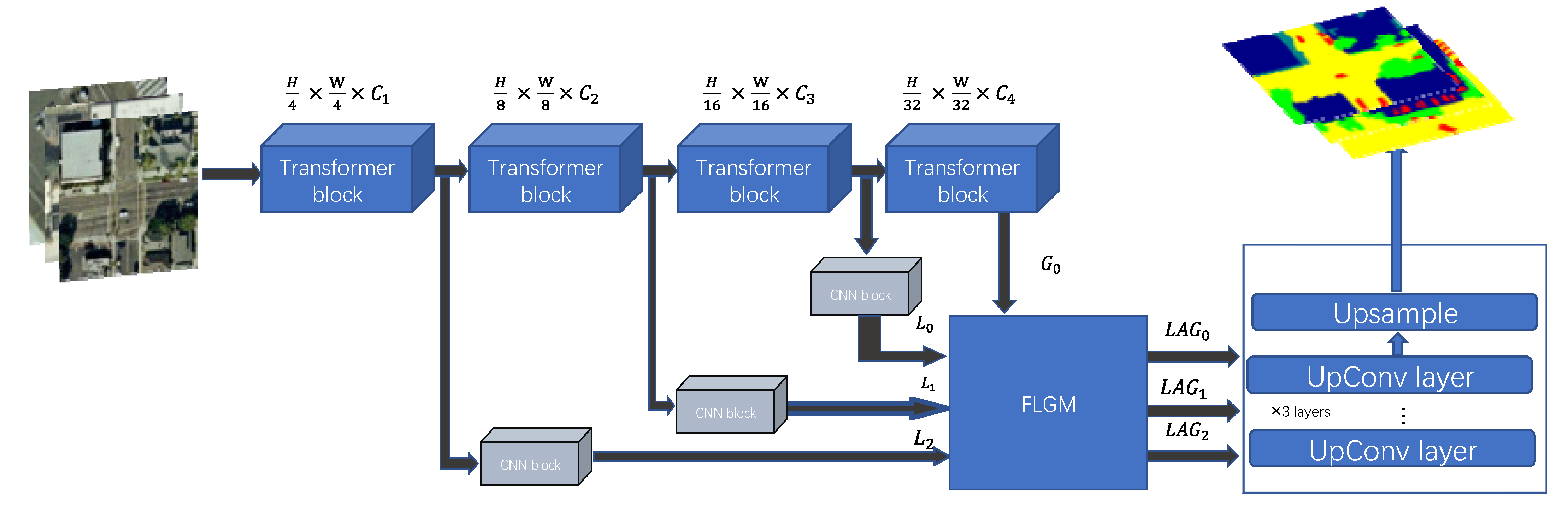
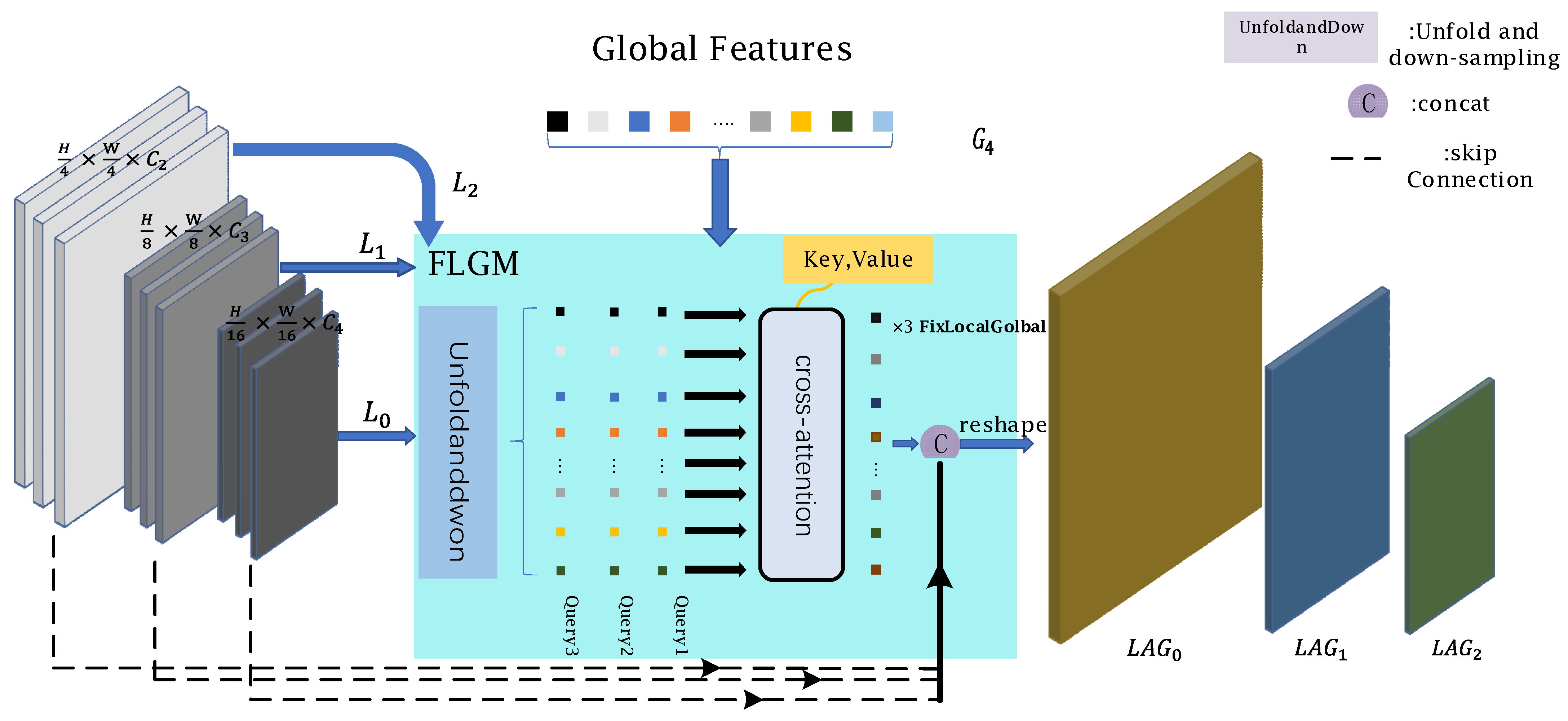
3.3. FLGM
| Algorithm 1 FLGM |
| #Description: cross: MutiHeadCrossAttention #Input: local_c is the local information that passes through the cnn branch #Input: G is the global information that passes through the transformer branch #Output: FixF is the local and global information fixed local_c = cnn(Loc_inf) #local information through cnn to get local_c = self.linear_c(local_c).permute(0,2,1).reshape(n,1, local_c.shape[2], local_c.shape[3]) Fix = rearrange(self.cross(local_c, G),’b (h w) c->b c h w’, h = local_c.size()[2]) #Repeat L time cross FixF = torch.cat([Fix, local_c],dim = 2) return FixF, G |
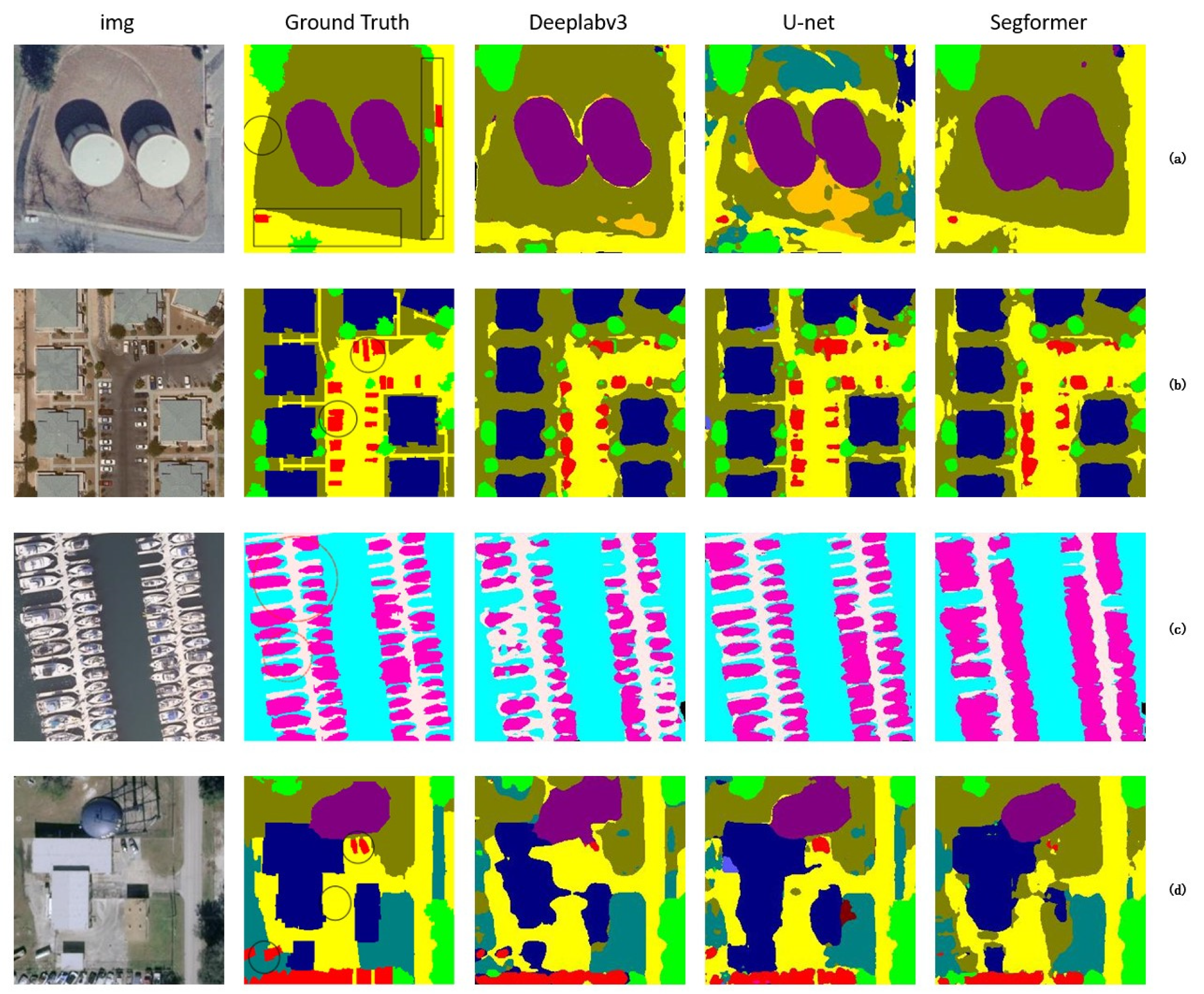
4. Experiment
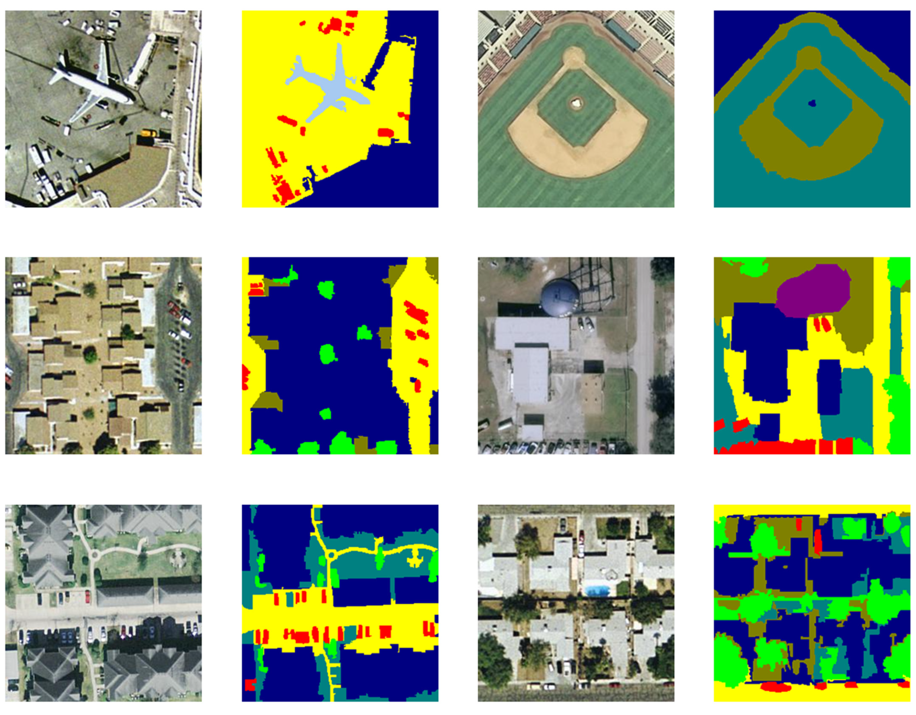
4.1. The Dataset
4.2. Evaluation Indicators
4.2.1. mPA (Mean Pixel Accuracy)
4.2.2. mIoU (Mean Intersection over Union)
4.2.3. Recall
4.2.4. Precision
4.2.5. mAccuracy
4.3. Implementation Detailed
Experimental Environment and Parameters
5. Conclusions
Author Contributions
Funding
Data Availability Statement
Conflicts of Interest
References
- Liu, X.; Cui, B.; Yan, S. Seed region growing based on gradient vector flow for medical image segmentation. Comput. Med. Imaging Graph. 2008, 32, 124–131. [Google Scholar]
- Oka, M.; Roy, R. Effective Image Segmentation using Fuzzy C Means Clustering with Morphological Processing. Int. J. Image Graph. Signal Process. 2012, 4, 49–56. [Google Scholar]
- Basse, R.M.; Omrani, H.; Charif, O.; Gerber, P.; Bódis, K. Land use changes modelling using advanced methods: Cellular automata and artificial neural networks. The spatial and explicit representation of land cover dynamics at the cross-border region scale. Appl. Geogr. 2014, 53, 160–171. [Google Scholar] [CrossRef]
- Krizhevsky, A.; Sutskever, I.; Hinton, G.E. Imagenet classification with deep convolutional neural networks. Commun. ACM 2017, 60, 84–90. [Google Scholar] [CrossRef]
- Deng, J.; Wei, D.; Socher, R.; Li, L.-J.; Li, K.; Li, F.-F. ImageNet: A large-scale hierarchical image database. In Proceedings of the IEEE Conference on Computer Vision and Pattern Recognition (CVPR), Miami, FL, USA, 20–25 June 2009; pp. 248–255. [Google Scholar]
- Jonathan, L.; Shelhamer, E.; Darrell, T. Fully convolutional networks for semantic segmentation. In Proceedings of the IEEE Conference on Computer Vision and Pattern Recognition, Santiago, Chile, 7–13 December 2015. [Google Scholar]
- Ronneberger, O.; Fischer, P.; Brox, T. U-net: Convolutional networks for biomedical image segmentation. In Medical Image Computing and Computer-Assisted Intervention–MICCAI 2015: 18th International Conference, Munich, Germany, 5–9 October 2015, Proceedings, Part III 18; Springer International Publishing: Berlin/Heidelberg, Germany, 2015. [Google Scholar]
- Chen, L.C.; Papandreou, G.; Kokkinos, I.; Murphy, K.; Yuille, A.L. Semantic image segmentation with deep convolutional nets and fully connected crfs. arXiv 2014, arXiv:1412.7062. [Google Scholar]
- Chen, L.C.; Papandreou, G.; Kokkinos, I.; Murphy, K.; Yuille, A.L. Deeplab: Semantic image segmentation with deep convolutional nets, atrous convolution, and fully connected crfs. IEEE Trans. Pattern Anal. Mach. Intell. 2017, 40, 834–848. [Google Scholar] [CrossRef]
- Chen, L.C.; Papandreou, G.; Schroff, F.; Adam, H. Rethinking atrous convolution for semantic image segmentation. arXiv 2017, arXiv:1706.05587. [Google Scholar]
- Chen, L.C.; Zhu, Y.; Papandreou, G.; Schroff, F.; Adam, H. Encoder-decoder with atrous separable convolution for semantic image segmentation. In Proceedings of the European Conference on Computer Vision (ECCV), Munich, Germany, 8–14 September 2018. [Google Scholar]
- Dai, J.; Qi, H.; Xiong, Y.; Li, Y.; Zhang, G.; Hu, H.; Wei, Y. Deformable convolutional networks. In Proceedings of the IEEE International Conference on Computer Vision, Venice, Italy, 22–29 October 2017. [Google Scholar]
- Liu, S.; Huang, D. Receptive field block net for accurate and fast object detection. In Proceedings of the European Conference on Computer Vision (ECCV), Munich, Germany, 8–14 September 2018. [Google Scholar]
- Yu, F.; Koltun, V. Multi-scale context aggregation by dilated convolutions. arXiv 2015, arXiv:1511.07122. [Google Scholar]
- Dosovitskiy, A.; Beyer, L.; Kolesnikov, A.; Weissenborn, D.; Zhai, X.; Unterthiner, T.; Dehghani, M.; Minderer, M.; Heigold, G.; Gelly, S.; et al. An image is worth 16 × 16 words: Transformers for image recognition at scale. arXiv 2020, arXiv:2010.11929. [Google Scholar]
- Liu, Z.; Lin, Y.; Cao, Y.; Hu, H.; Wei, Y.; Zhang, Z.; Lin, S.; Guo, B. Swin transformer: Hierarchical vision transformer using shifted windows. In Proceedings of the IEEE/CVF International Conference on Computer Vision, Montreal, QC, Canada, 10–17 October 2021; pp. 10012–10022. [Google Scholar]
- Xie, E.; Wang, W.; Yu, Z.; Anandkumar, A.; Alvarez, J.M.; Luo, P. SegFormer: Simple and efficient design for semantic segmentation with transformers. Adv. Neural Inf. Process. Syst. 2021, 34, 12077–12090. [Google Scholar]
- Vaswani, A.; Shazeer, N.; Parmar, N.; Uszkoreit, J.; Jones, L.; Gomez, A.N.; Kaiser, Ł.; Polosukhin, I. Attention is all you need. In Advances in Neural Information Processing Systems 30, Proceedings of the 31th International Conference on Neural Information Processing Systems, Long Beach, CA, USA, 4–9 December 2017; Curran Associates Inc.: Red Hook, NY, USA, 2017. [Google Scholar]
- Devlin, J.; Chang, M.W.; Lee, K.; Toutanova, K. Bert: Pre-training of deep bidirectional transformers for language understanding. arXiv 2018, arXiv:1810.04805. [Google Scholar]
- Carion, N.; Massa, F.; Synnaeve, G.; Usunier, N.; Kirillov, A.; Zagoruyko, S. End-to-end object detection with transformers. In Computer Vision–ECCV 2020: 16th European Conference, Glasgow, UK, 23–28 August 2020, Proceedings, Part I 16; Springer International Publishing: Berlin/Heidelberg, Germany, 2020; pp. 213–229. [Google Scholar]
- Guo, M.-H.; Lu, C.-Z.; Liu, Z.-N.; Cheng, M.-M.; Hu, S.-M. Visual attention network. arXiv 2022, arXiv:2202.09741. [Google Scholar]
- Xu, D.; Alameda-Pineda, X.; Ouyang, W.; Ricci, E.; Wang, X.; Sebe, N. Probabilistic graph attention network with conditional kernels for pixel-wise prediction. IEEE Trans. Pattern Anal. Mach. Intell. 2020, 44, 2673–2688. [Google Scholar] [CrossRef]
- Cortes, C.; Vapnik, V. Support-Vector Networks. Mach. Learn. 2003, 20, 273–297. [Google Scholar] [CrossRef]
- Breiman, L. Random forests. Mach. Learn. 2001, 45, 5–32. [Google Scholar] [CrossRef]
- Volpi, M.; Tuia, D. Deep multi-task learning for a geographically-regularized semantic segmentation of aerial images. ISPRS J. Photogramm. Remote Sens. 2018, 144, 48–60. [Google Scholar] [CrossRef]
- Marmanis, D.; Wegner, J.D.; Galliani, S.; Schindler, K.; Datcu, M.; Stilla, U. Semantic segmentation of aerial images with an ensemble of CNSS. ISPRS Ann. Photogramm. Remote Sens. Spat. Inf. Sci. 2016, 3, 473–480. [Google Scholar] [CrossRef]
- Shao, Z.; Yang, K.; Zhou, W. Performance Evaluation of Single-Label and Multi-Label Remote Sensing Image Retrieval Using a Dense Labeling Dataset. Remote Sens. 2018, 10, 964. [Google Scholar] [CrossRef]
- Waldner, F.; Diakogiannis, F.I. Deep learning on edge: Extracting field boundaries from satellite images with a convolutional neural network. Remote Sens. Environ. 2020, 245, 111741. [Google Scholar] [CrossRef]
- Ding, L.; Zhang, J.; Bruzzone, L. Semantic segmentation of large-size VHR remote sensing images using a two-stage multiscale training architecture. IEEE Trans. Geosci. Remote Sens. 2020, 58, 5367–5376. [Google Scholar] [CrossRef]
- Liu, R.; Li, M.; Chen, Z. AFNet: Adaptive fusion network for remote sensing image semantic segmentation. IEEE Trans. Geosci. Remote Sens. 2020, 59, 7871–7886. [Google Scholar] [CrossRef]
- Liu, Z.; Mao, H.; Wu, C.-Y.; Feichtenhofer, C.; Darrell, T.; Xie, S. A ConvNet for the 2020s. In Proceedings of the 2022 IEEE/CVF Conference on Computer Vision and Pattern Recognition (CVPR), New Orleans, LA, USA, 18–24 June 2022. [Google Scholar] [CrossRef]
- Xie, S.; Girshick, R.; Dollár, P.; Tu, Z.; He, K. Aggregated residual transformations for deep neural networks. In Proceedings of the IEEE Conference on Computer Vision and Pattern Recognition, Honolulu, HI, USA, 21–26 July 2017; pp. 1492–1500. [Google Scholar]
- Heraa, S.; Gong, J. Transformer-Based Deep Learning Model for SAR Image Segmentation. In Proceedings of the 2021 International Conference on Intelligent Transportation, Big Data & Smart City, Xi’an, China, 27–28 March 2021; pp. 166–173. [Google Scholar]
- Zhao, H.; Shi, J.; Qi, X.; Wang, X.; Jia, J. Pyramid scene parsing network. In Proceedings of the IEEE Conference on Computer Vision and Pattern Recognition, Honolulu, HI, USA, 21–26 July 2017. [Google Scholar]
- Zhao, H.; Qi, X.; Shen, X.; Shi, J.; Jia, J. Icnet for real-time semantic segmentation on high-resolution images. In Proceedings of the European Conference on Computer Vision (ECCV), Munich, Germany, 8–14 September 2018. [Google Scholar]
- Ba, J.L.; Kiros, J.R.; Hinton, G.E. Layer normalization. arXiv 2016, arXiv:1607.06450. [Google Scholar]
- Ghiasi, G.; Lin, T.-Y.; Le, Q.V. Dropblock: A regularization method for convolutional networks. In Advances in Neural Information Processing Systems 31, Proceedings of the 32th International Conference on Neural Information Processing Systems, Montreal, QC, Canada, 3–8 December 2018; Curran Associates Inc.: Red Hook, NY, USA, 2018. [Google Scholar]
- Bastidas, A.A.; Tang, H. Channel attention networks. In Proceedings of the IEEE/CVF Conference on Computer Vision and Pattern Recognition Workshops, Long Beach, CA, USA, 16–17 June 2019. [Google Scholar]
- Li, Z.; Chen, Z.; Liu, X.; Jiang, J. Depthformer: Exploiting long-range correlation and local information for accurate monocular depth estimation. arXiv 2022, arXiv:2203.14211. [Google Scholar]
- Howard, A.G.; Zhu, M.; Chen, B.; Kalenichenko, D.; Wang, W.; Weyand, T.; Andreetto, M.; Adam, H. Mobilenets: Efficient convolutional neural networks for mobile vision applications. arXiv 2017, arXiv:1704.04861. [Google Scholar]
- Wang, J.; Zheng, Z.; Ma, A.; Lu, X.; Zhong, Y. LoveDA: A remote sensing land-cover dataset for domain adaptive semantic segmentation. arXiv 2021, arXiv:2110.08733. [Google Scholar]
- Loshchilov, I.; Hutter, F. Decoupled weight decay regularization. arXiv 2017, arXiv:1711.05101. [Google Scholar]


| Prediction Results | ||
|---|---|---|
| Positive | Negative | |
| Positive | True Positive (TP) | False Negative (FN) |
| Negative | False Positive (FP) | True Negative (TN) |
| Model | Freeze Epoch | Epoch | Batch Size | Optimizer Tpye | Momentum | Weight Decay | Init lr/min lr | Lr Decay Type | FLOPs | Params |
|---|---|---|---|---|---|---|---|---|---|---|
| U-net | 100 | 200 | 16 | Sgd | 0.9 | 1 × 10⁻⁴ | 7 × 10⁻³/7 × 10−3 × 0.01 | cos | 56.52 G | 24.89 M |
| DeepLabV3 | 100 | 200 | 16 | Sgd | 0.9 | 1 × 10⁻⁴ | 7 × 10⁻³/7 × 10−3 × 0.01 | cos | 112.87 G | 23.71 M |
| Segformer | 100 | 200 | 16 | AdamW | 0.9 | 1 × 10⁻² | 1 × 10⁻⁵/1 × 10−5 × 0.01 | cos | 28.38 G | 27.35 M |
| 100 | 200 | 16 | AdamW | 0.9 | 1 × 10⁻² | 1 × 10⁻⁵/1 × 10−5 × 0.01 | cos | 21.44 G | 20.76 M |
| Model | mIoU | mPA | mAccuracy | MRecall | mPrecision |
|---|---|---|---|---|---|
| U-net | 71.59% | 83.36% | 86.16% | 82.45% | 83.80% |
| DeepLabV3 | 70.40% | 83.36% | 86.59% | 83.36% | 81.28% |
| Segformer | 72.97% | 85.63% | 89.68% | 85.63% | 82.62% |
| 75.32% | 86.04% | 90.78% | 86.04% | 85.11% |
| DLRSD IOU | |||||||||||||||||
|---|---|---|---|---|---|---|---|---|---|---|---|---|---|---|---|---|---|
| Category | Water | Trees | Tanks | Ships | Sea | Sand | Pavement | Mobile Home | Grass | Filed | Dock | Court | Chaparral | Cars | Buildings | Bare Soil | Airplane |
| DeepLabV3 | 0.80 | 0.72 | 0.77 | 0.71 | 0.91 | 0.65 | 0.78 | 0.63 | 0.55 | 0.96 | 0.53 | 0.71 | 0.65 | 0.65 | 0.69 | 0.58 | 0.68 |
| U-net | 0.78 | 0.74 | 0.82 | 0.78 | 0.94 | 0.58 | 0.76 | 0.64 | 0.54 | 0.94 | 0.60 | 0.76 | 0.71 | 0.70 | 0.65 | 0.54 | 0.70 |
| Segformer | 0.81 | 0.77 | 0.76 | 0.72 | 0.92 | 0.69 | 0.81 | 0.65 | 0.62 | 0.97 | 0.51 | 0.82 | 0.65 | 0.65 | 0.76 | 0.61 | 0.67 |
| 0.83 | 0.79 | 0.84 | 0.75 | 0.92 | 0.73 | 0.83 | 0.70 | 0.64 | 0.98 | 0.58 | 0.83 | 0.58 | 0.68 | 0.79 | 0.61 | 0.73 | |
| DLRSD PA | |||||||||||||||||
|---|---|---|---|---|---|---|---|---|---|---|---|---|---|---|---|---|---|
| Category | Water | Trees | Tanks | Ships | Sea | Sand | Pavement | Mobile Home | Grass | Filed | Dock | Court | Chaparral | Cars | Buildings | Bare Soil | Airplane |
| DeepLabV3 | 0.88 | 0.84 | 0.94 | 0.79 | 1.00 | 0.76 | 0.86 | 0.78 | 0.73 | 0.96 | 0.71 | 0.96 | 0.82 | 0.79 | 0.77 | 0.75 | 0.84 |
| U-net | 0.86 | 0.89 | 0.91 | 0.84 | 0.99 | 0.68 | 0.89 | 0.83 | 0.63 | 0.95 | 0.74 | 0.93 | 0.78 | 0.83 | 0.76 | 0.72 | 0.77 |
| Segformer | 0.90 | 0.89 | 0.95 | 0.90 | 1.00 | 0.77 | 0.89 | 0.87 | 0.74 | 0.97 | 0.64 | 0.97 | 0.82 | 0.78 | 0.87 | 0.74 | 0.87 |
| 0.91 | 0.89 | 0.95 | 0.88 | 0.99 | 0.76 | 0.91 | 0.86 | 0.77 | 0.98 | 0.73 | 0.96 | 0.72 | 0.80 | 0.88 | 0.76 | 0.87 | |
| LoveDA-Urban | |||||
|---|---|---|---|---|---|
| mIoU | mPA | mAccuracy | MRecall | mPrecision | |
| Deeplabv3 | 66.20% | 77.29% | 77.13% | 77.29% | 80.24% |
| U-net | 65.38% | 78.48% | 76.02% | 78.48% | 77.62% |
| Segformer | 67.75% | 80.06% | 77.71% | 80.06% | 79.81% |
| 69.94% | 80.55% | 79.57% | 80.55% | 82.62% | |
| Agriculture | Forest | Barren | Water | Road | Building | Background | |
|---|---|---|---|---|---|---|---|
| Deeplabv3 | 0.55 | 0.52 | 0.53 | 0.84 | 0.62 | 0.60 | 0.64 |
| U-net | 0.56 | 0.51 | 0.48 | 0.84 | 0.62 | 0.61 | 0.61 |
| Segformer | 0.59 | 0.53 | 0.56 | 0.86 | 0.64 | 0.61 | 0.64 |
| 0.62 | 0.56 | 0.58 | 0.88 | 0.66 | 0.63 | 0.67 |
Disclaimer/Publisher’s Note: The statements, opinions and data contained in all publications are solely those of the individual author(s) and contributor(s) and not of MDPI and/or the editor(s). MDPI and/or the editor(s) disclaim responsibility for any injury to people or property resulting from any ideas, methods, instructions or products referred to in the content. |
© 2023 by the authors. Licensee MDPI, Basel, Switzerland. This article is an open access article distributed under the terms and conditions of the Creative Commons Attribution (CC BY) license (https://creativecommons.org/licenses/by/4.0/).
Share and Cite
Zhang, Z.; Liu, B.; Li, Y. FURSformer: Semantic Segmentation Network for Remote Sensing Images with Fused Heterogeneous Features. Electronics 2023, 12, 3113. https://doi.org/10.3390/electronics12143113
Zhang Z, Liu B, Li Y. FURSformer: Semantic Segmentation Network for Remote Sensing Images with Fused Heterogeneous Features. Electronics. 2023; 12(14):3113. https://doi.org/10.3390/electronics12143113
Chicago/Turabian StyleZhang, Zehua, Bailin Liu, and Yani Li. 2023. "FURSformer: Semantic Segmentation Network for Remote Sensing Images with Fused Heterogeneous Features" Electronics 12, no. 14: 3113. https://doi.org/10.3390/electronics12143113
APA StyleZhang, Z., Liu, B., & Li, Y. (2023). FURSformer: Semantic Segmentation Network for Remote Sensing Images with Fused Heterogeneous Features. Electronics, 12(14), 3113. https://doi.org/10.3390/electronics12143113