Review

Constructing Maps for Autonomous Robotics: An Introductory Conceptual Overview

Institute of Electronics and Computer Science, LV-1006 Riga, Latvia
*
Authors to whom correspondence should be addressed.
Electronics 2023, 12(13), 2925; https://doi.org/10.3390/electronics12132925
Submission received: 14 June 2023 / Revised: 26 June 2023 / Accepted: 29 June 2023 / Published: 3 July 2023
(This article belongs to the Special Issue Autonomous Robots and Systems)

Abstract

:
Mapping the environment is a powerful technique for enabling autonomy through localization and planning in robotics. This article seeks to provide a global overview of actionable map construction in robotics, outlining the basic problems, introducing techniques for overcoming them, and directing the reader toward established research covering these problem and solution domains in more detail. Multiple levels of abstraction are covered in a non-exhaustive vertical slice, starting with the fundamental problem of constructing metric occupancy grids with Simultaneous Mapping and Localization techniques. On top of these, topological meshes and semantic maps are reviewed, and a comparison is drawn between multiple representation formats. Furthermore, the datasets and metrics used in performance benchmarks are discussed, as are the challenges faced in some domains that deviate from typical laboratory conditions. Finally, recent advances in robot control without explicit map construction are touched upon.

1. Introduction

While stationary industrial robot manipulators can be programmed to execute a specific task without reference to their external environment, perception is critical for interacting with dynamic environments [1]. In the context of mobile robotics, this often (though not always [2]) requires the construction of a map, which is readily apparent in the interfaces for widely-used navigation and planning packages [3]. For solving more complex tasks, the extension of basic spatial obstacle maps with topological structure [4] and semantic information [5] has been an active area of research for multiple decades now.
Constructing a high-level map, such as in [6] or [7], involves multiple steps, each of which traditionally constitutes a distinct research niche on its own. At the lower level of many systems, one can find a Simultaneous Localization and Mapping (SLAM) solver, concerned with the problem of estimating the robot state with a map, while also constructing the very same map with respect to these state estimates. This in itself is a large and active area of research, with detailed expositions [8,9] and surveys [10,11] available. However, these typically make no mention of the higher-level aspects of mapping. Meanwhile, while some exhaustive surveys concerned with these more abstract levels exist [12], these tend to assume that the reader is already familiar with SLAM or mention it only in passing—even though these high- and low-level concepts are not always neatly separable [13]. In this article, we seek to bridge the gap by describing the entire mapping stack, avoiding off-hand references to concepts new researchers entering the field may be unfamiliar with, as a starting point for more detailed reading. Thus, with this overview, we do not seek to exhaustively review any of the research areas discussed but rather introduce key concepts, terminology, and seminal works which would lead one to more quickly uncover the state of the art in their particular question of interest.
The structure of this article is primarily motivated by the gulf in the literature between covering the low-level implementation of SLAM and the ways in which higher-level map construction capabilities may be grafted onto a SLAM system. Examples abound of a SLAM system [14] serving as the basis for multiple, potentially very different high-level mapping systems [7,15]. Therefore, we choose to make the first distinction at this divide—with Section 2 covering the lower-level problem of SLAM. We further break down the SLAM problem according to the two ways of posing it, as local filtering or tracking, only considering the last state, and global smoothing, optimizing over the entire past history of states. In part to show how these may be tied together, we then include examples of real systems, some of which utilize the two-stage tracking-mapping approach which has become commonplace.
Section 3 addresses the questions of map representations, ways to convert between them, and how additional information—not part of the SLAM process—may be integrated. Specifically, the subsections of Section 3 loosely follow the metric–topological–semantic hierarchy of environment mapping that has been pervasive in the field of autonomous robotics for many decades before practicable SLAM systems became available [4,5]. Taken as a whole, these two sections should give the reader a grasp on the terminology and concepts required to make sense of articles covering proposed SLAM and multi-level mapping approaches for robotics.
While the first two sections are concerned with actually solving the various problems described, Section 4 discusses the perhaps equally important question of how one can go about evaluating solutions, briefly covering the data and metrics used in various benchmarks. Finally, some adjacent questions which do not neatly fit under the main contents of this overview—domain-specific challenges that require deviations from more typical approaches, and the prospect of autonomous robotics without explicit, human-readable maps—are covered in Section 5.

2. Building Maps—Core Concepts in SLAM

Before discussing higher-level map construction, it is necessary to have a thorough grasp of the Simultaneous Localization and Mapping (SLAM) problem, which is what enables a robot to have a consistent picture of its surroundings in the absence of external ground truth positioning data in the first place. This is a broad and deep topic, a detailed, first principles exposition of which can be found in Probabilistic Robotics by Thrun et. al. [8]. This book, in addition to covering the mathematical foundations of probabilistic motion and observation models, introduces both of the commonly found approaches to solving the SLAM problem, filtering, notably by means of an Extended Kalman Filter (EKF), and smoothing, which is described in terms of the Extended Information Filter (EIF), in the book.
The latter approach has grown much more popular in the following decades, becoming strongly associated with the factor graph formalism in the process, so readers primarily interested in smoothing-based methods may find Factor Graphs for Robot Perception by Dellaert and Kaess [9] to be more helpful. This extended article describes and motivates factor graphs as a tool for posing and solving a variety of non-linear optimization problems, placing an emphasis on SLAM in particular. Specifically, after explaining how to solve the problem in steps, the ways one can exploit sparsity in the problem structure to reduce computational complexity are covered. Additionally, useful information on the mathematical tools employed is provided, for example, the employment of Lie Algebras in optimization over manifolds, which arises when optimizing over rotations in S O ( 2 ) or S O ( 3 ) .
Bearing in mind the existence of detailed resources, such as the ones described above, this section consists of a brief description of the core concepts in SLAM, followed by a short list of implementation examples.

2.1. Problem Formulation, Concepts

2.1.1. Full SLAM

When formally posed in the broadest possible sense [8], the full SLAM problem can be stated as maximizing the joint posterior
p ( x 1 : t , m | z 1 : t , u 1 : t )
over a sequence x 1 : t of robot states x t , a map representation of the environment m, with sequences of sensor observation constraints z t and odometry constraints u t (also known as controls, assuming these are known inputs to the robot control system). The map is frequently given by a list of landmarks l i , though the representations of these may vary widely based upon the sensor modality and algorithm employed. Particularly, in a smoothing context [9], the robot state history x k : t and environment map m may also be considered a single state vector X which concatenates the minimum degree of freedom descriptions of each. Generally, one also needs a state propagation function (movement model) p ( x t | x t 1 , u t ) = g ( x , u ) and observation model p ( z t | x t , l i ) = h ( x , l ) . Note that the latter depends on making correct associations between landmarks and observations, which is known as the correspondence problem in SLAM, and is typically implicit in the notation used to describe algorithms.
A single robot state x t is generally a pose—a concatenation of position (translation) t and orientation (rotation) R. t may belong to R 2 or R 3 for position in 2D or 3D space, respectively, while the corresponding R is typically a matrix in S O ( 2 ) or S O ( 3 ) —the special orthogonal groups consisting of orthogonal 2 × 2 and 3 × 3 matrices with determinant 1. The Cartesian product R n × S O ( n ) then constitutes the n-dimensional special Euclidean group S E ( n ) , with composition:
( R 1 , t 1 ) ( R 2 , t 2 ) = ( R 1 R 2 , R 1 t 2 + t 1 )
Often, S E ( n ) is expressed in terms of an n + 1 × n + 1 projective transform matrix
T = ( R , t ) = R t 0 1 ,
with inversion and composition defined as
T 1 = R T R T t 0 1
T 1 T 2 = T 1 T 2 = R 1 R 2 R 1 t 1 + t 1 0 1
also giving rise to the relative pose
T i j = T j 1 T i T i = T j ( T j 1 T i ) = T j T i j
which, when obtained as a constraint between two subsequent poses in a trajectory, is generally known as the odometry, but a loop closure when introduced by some other data association method.
The states of landmark features l making up the map m have much more varied representations, such as the positions of geometric features extracted from LiDAR point clouds in a global coordinate system [16] to range and bearing estimates for photometric features in the latest robot coordinate frame [17], making any kind of general treatment impracticable. If the system is only concerned with estimating the current pose of the robot, it may discard landmarks after they pass out of bounds in the current local reference frame, resulting in an odometry or tracking algorithm, rather than a full SLAM system [17,18,19]. It is, however, not uncommon for such a tracking algorithm to form part of a full SLAM system by producing initial estimates for map features and robot state histories, which can subsequently be refined in a global mapper [20,21,22,23].
It is important to note that the set of landmarks in the map need not constitute the sum total of sensor measurements, only those utilized in localizing the robot. Assuming an accurate robot trajectory is available—regardless of whether it was produced by a local tracking or full SLAM algorithm—a map can be obtained by means like integrating back-projected ranging sensor measurements, as discussed in chapter 9 of [8], or using the photogrammetric reconstruction techniques extensively described in [24]. The outputs of this process are discussed in more detail in Section 3.1.

2.1.2. Filter SLAM

The filter SLAM differs formally in that only the most recent state of the robot is estimated [8]
p ( x t , m | z 1 : t , u 1 : t ) ,
which has several important implications:
  • This makes the problem more tractable for algorithms in the form of a Bayes filter, which operate by iterated repetition of a state transition function followed by a measurement update. Note that probability distributions over hidden states x are referred to as belief  bel ( x ) in [8] and works derived thereof.
  • Prior state estimates are marginalized out, with information about them being contained in the beliefs over landmarks and current state. When dealing with non-linear state propagation and observation functions, this means that re-linearization of these functions cannot be performed, contributing to drift.
  • There is a strong distinction between odometry and measurement constraints, in that the former is used in the state propagation step and the latter in measurement updates.
The second point, in particular, contributes to this formulation being more suited for tracking or odometry applications than extensive map construction [17,19,25]. Though a variety of parametric and non-parametric distributions may be used in a Bayes filter, when one assumes the combined state vector X is normally distributed with mean x t , covariance Σ t , state transition g ( x , u ) , and observation g ( x ) , it is an instance of the Extended Kalman Filter (EKF), an explanation and derivation of which can be found in [8]. While practical implementations may differ in using an iterated [19] or multi-state [25] formulation of the filter, or process incoming Inertial Measurement Unit (IMU) odometry data at a separate rate from the measurement updates conducted by external sensors (namely, camera images) [17], the incremental linearization of g ( x , u ) and h ( x ) is apparent in all cases.
Particularly when tackled in the context of a tracking front-end for a global mapping back-end, as in [20,21,22,23], the filter SLAM problem may also be formulated as a smoothing problem over a history of recent poses and landmark observations. Since non-local information is marginalized out, a smoothing tracker suffers from the same linearization drift as an explicit Bayes filter.

2.1.3. Smoothing SLAM and Factor Graphs

Factor graphs offer perhaps the most concise and straightforward way to reason about the smoothing approach to SLAM [9,26]. Given a posterior distribution which is proportional to a product of factors
p ( X ) ϕ ( X ) = i ϕ i ( X i ) ,
the factor graph F is an undirected bipartite graph with variable vertices x i X , factor vertices ϕ i Φ and edges { e } = { x j , ϕ i } | x j X i . Maximizing the posterior—smoothing—is then equivalent to maximizing the product of the factors:
X M A P = arg max X i ϕ i ( X i )
The factors can take on arbitrary form, for example, non-parametric kernel density estimators [27]. However, it is very common to assume Gaussian factors, as evidenced by the default choices made in popular factor graph optimization software [28]. These consist of an observation constraint N ( z i , Σ i ) and a (generally non-linear) function h ( x i ) relating this to some subset of state variables [9], giving the form
ϕ ( X ) = i η i exp 1 2 h ( x i ) z i Σ i 2
which results in the following sparse non-linear least squares problem
arg max X i ϕ i ( X i ) = arg min X i h ( x i ) z i Σ i 2
arg min Δ X i h ( x 0 ) + H i Δ x i z i Σ i 2 =
= arg min Δ X i Σ i 1 / 2 H i A i Δ x i Σ i 1 / 2 [ z i h ( x 0 ) ] b i ) 2 =
= arg min Δ X A Δ X b 2
where the combined Jacobian-square root information matrix A has a sparse block structure corresponding to the individual factor Jacobians H i . In the general case, this can be solved by methods such as the iterative Gauss–Newton algorithm
A i T A i Δ X i + 1 = A i T b i
Given that the matrix A T A is positive-definite, the above can then be solved using, e.g., Cholesky decomposition into upper-lower triangular matrices R , R T
A T A = R T R R T y = b R Δ X = y
While exploring the computational complexity of matrix algebra is beyond the scope of this work, given the inherent sparsity of A, solutions can be found much faster than the theoretical O ( n 3 ) complexity of matrix inversion suggests, using the elimination algorithm for decomposition. Further speed-ups can be attained by manipulating the order of variables to minimize fill-in (the fraction of non-zero off-diagonal elements). Ref. [9] explores these considerations in detail and shows examples of using information about problem structure contained in factor graphs to achieve linear speed-ups over domain-agnostic sparse linear algebra solvers.
An important thing to note here is that h ( x ) can take on different forms to suit a variety of observation modalities. If only relative pose constraints (odometries and loop closures) between robot poses are available, this is known as a pose graph optimization (PGO) problem. This can quite frequently be seen in global mapping back-ends, which receive pose constraints and initial estimates from a tracking front-end [16,23,29]. In such systems, a local mapping/tracking thread periodically produces a keyframe and inserts it into the global pose graph. Typically, a descriptor of each keyframe (e.g., [30]) will also be computed, against which new keyframes are compared to find potential loop closures.
However, factors relating robot poses to landmark features are also widely used, especially when performing tracking over a limited history of poses [23]. For example, in purely visual SLAM, such as [21], landmarks may take the form of image feature descriptors (used for data association frame-to-frame), a spatial position, and constraints for viewing angle and distance. The cost function to minimize may then take on the form of a reprojection error
x i l j : z i j π ( l j , x i ) z i j Σ i j 2
where x i are robot (camera) poses, ( z i j , Σ i j ) are observation factors (distributions over 2D pixel coordinates), π is some function projecting landmarks into the image coordinate system, and l j are the landmarks associated with z i j by a data association algorithm, such as feature descriptor matching or optical flow tracking. In isolation this is then known as bundle adjustment (BA), and, provided no additional factor types are included in the graph, makes this equivalent to the Structure from Motion (SfM) problem from photogrammetry [31].
The utility of using the factor graph formalism for describing optimization problems becomes apparent when multiple types of factors are considered at once. A typical case is the combination of feature observation factors with odometry constraints obtained from an IMU [20,22,23]. Figure 1 illustrates how the different types of constraints can be readily combined into a single structure. As IMU data rates are generally much greater than camera framerates, IMU constraints are typically given as pre-integrated odometry factors between robot poses taken at the camera framerate, combining dozens or hundreds of individual measurements using the method formalized in [32]. This gives rise to the structure illustrated in the bottom factor graph of Figure 1.

2.2. Representative Examples

With blurry distinctions between tracking/odometry and full SLAM, filtering and smoothing, sensor modalities, and combinations thereof, literature on SLAM defies attempts at drafting trivial taxonomies. An exhaustive description of the state of the art in SLAM is also not the primary focus of this article. For more detailed surveys about visual SLAM in particular and SLAM in general we direct the reader to [10] and [11], respectively. What follows is a short list of representative examples, which illustrate how the concepts discussed in the previous subsection may be applied in practice. Table 1 collates the key distinctions between these systems in a concise format.
ORB-SLAM (2015) by Mur-Artal et. al. [21] is not the first to employ the two-stage tracking–mapping architecture so common in modern SLAM systems, with much earlier implementations, such as PTAM [38]; however, it serves as a good example of a practically useful smoothing-based monocular SLAM system. Fundamentally, the entire approach is based on three threads executing in parallel—tracking, local mapping, and global optimization. On all levels, ORB descriptors [39] are used to identify image features, and each feature is associated with a map point. The bag-of-words descriptors of keyframes [30] are computed and stored in a database for rapid similarity-based look-up.
Tracking is performed in two steps. The first searches for correspondences with the previous frame and uses those to optimize an initial estimate based on extrapolated velocity. Should tracking fail, relocalization is performed by bag-of-words look-up and corresponding optimization. The second step expands the number of map features used by including all points in the local map, defined by a two-degree covisibility graph over keyframes (neighbor-of-neighbor by shared features), and optimizes the current pose again. The decision to insert a new keyframe is based on a heuristic.
Mapping is handled in two threads. Local mapping is performed whenever a new keyframe is inserted. Using the same covisibility graph, a subset of keyframes and map features are selected for optimization. The new frame is inserted into the map along with a reduced set of novel map points, and bundle adjustment is performed, this time optimizing all the parameters in the local map. Finally, a loop closing thread runs in the background, searching for correspondences using bag-of-words and introducing loop closures. A spanning tree of the covisibility graph is maintained for inter-frame relative pose constraints, and this is used for pose graph optimization when adding loop closures.
An inherent drawback of monocular SLAM is the scale ambiguity. Without additional constraints, such as known spatial distances between points in an image, projective geometry can only recover similarity transforms between camera poses, with an additional degree of freedom [24]. Furthermore, this greatly complicates the bootstrapping of the mapping process with initial estimates, and a considerable amount of attention in [21] is given to robust initialization of the map. While there have been attempts to alleviate these problems by directly inferring spatial information from the monocular image data using machine learning [18], many elect, instead, to overcome this issue by introducing an additional—inertial—source of measurement constraints to the localization estimates.
ORB-SLAM3 (2020) by Campos and Elvira et al. [22] is a continuation of the above. A number of evolutionary improvements notwithstanding, the most salient differences are using pre-integrated IMU constraints, stereo capability, and an atlas of multiple inactive maps that can be dynamically linked to the current one. As before, a three-thread structure is employed with tracking, local mapping, and loop closures. The IMU data enable the recovery of scale information, provide for better initial pose estimates, and enable much more rapid initialization of the map. Maintaining a database of offline maps makes the system inherently robust against complete tracking loss—should the robot fail to relocalize, it simply starts a new map. When correspondences between the current map and offline maps are discovered, they can be combined. While this is the system we chose to compare and contrast with the purely monocular approach above, given their great degree of similarity, one must also note that numerous fundamentally similar approaches exist, e.g., VINS-Mono [23], which has a comparable multi-threaded local-global mapping architecture, though only performing PGO in 4 degrees of freedom (courtesy of a consistent gravity direction).
Google Cartographer (2016) by Hess et. al. [33] offers a view into what the application of many of the same design principles leads to when used with a vastly different sensor data modality—LiDAR scans. Again, a tracking–mapping approach is used. However, the local maps—called submaps—are explicitly constructed from a number of subsequent LiDAR scans in the form of an occupancy grid map (OGM), detailed in Section 3.1.1. Each new scan first has its pose optimized with respect to the local submap, then is used to update the submap. The submaps, along with their scans, are periodically added to a global pose graph. Loop closures are found by looking for matches between scans and other submaps using a branch-and-bound algorithm, which is perhaps the main innovation of this system. These are then integrated into the state estimate by periodic pose graph optimization. Others have instead used frame descriptor-based place matching for this purpose [16] as in the visual examples discussed above.
iSAM2 (2012) by Kaess et. al. [40] explicitly seeks to address the issue largely skirted by previously mentioned smoothing approaches—the unbounded growth in problem size as more data are accumulated in the map. To address this, they introduce the Bayes tree, a data structure produced by applying the elimination algorithm to a factor graph [9], and refactoring the resulting chordal Bayes net, which is also equivalent to the Cholesky decomposition R discussed in Section 2.1. The tree structure exposes precisely the subset of variables that need to be relinearized and optimized whenever a new factor is introduced, and these contribute to generally greatly reduced problem sizes for any given modification to the global state estimate.
Maplab (2017) by Schneider et. al. [34] is an example backing the bold statement made in Section 2.1 that, in principle, a tracking algorithm is sufficient to produce maps. Specifically, they present a software package that uses the EKF-based ROVIO visual-inertial odometry system [17] to produce trajectories, from which maps can be constructed. These can then be optimized and fused with other maps using offline implementations of data association and smoothing algorithms.
Point-based Fusion (2013) by Keller et al. [35] is an RGB-D (depth image) SLAM system that serves as the basic mapping component in numerous other, wildly divergent approaches, e.g., [7,15,36], and, therefore, deserves a mention in our short list of examples. This system maintains a map in the form of an unordered list of surface features (surfels), discussed in Section 3.1.2. New camera poses are estimated by projecting the model points from the previous camera pose and performing iterative closest point (ICP) alignment with the current depth map. The points obtained from the current depth map are then back-projected and merged with the model using distance and confidence-based heuristics.
iMap (2021) by Sucar et al. [37] bridges the gap between classic non-linear least squares optimization and modern deep learning in SLAM. At the core of their approach is the neural radiance field (NRF) [41]—an implicit scene representation discussed in more detail in Section 3.1.3. The key difference from traditional methods is the replacement of “meaningful” parameters in the map model—such as a cloud of image features associated with spatial coordinates and viewing angles—with completely generic neural network weights and biases, of which there is a constant number. The neural network is parametrized by spatial coordinates and pixel value estimates can be recovered by the integration along projection rays described in [41]. This system and its derivatives [42] use RGB-D inputs in tracking and mapping. Model architecture aside, this approach is otherwise analogous to more traditional ones like [21,22,23,35]. Tracking is performed by optimizing the pose of the latest frame with regard to a frozen model. Smoothing is performed by jointly optimizing the pose graph and scene model over a set of keyframes using gradient descent.

2.3. Summary

Simultaneous Localization and Mapping (SLAM) is the problem of constructing a consistent map of the environment which can be used to localize the robot, while relying purely on sensor observations, without a reliable source of positioning information. Traditionally, it has been formulated in terms of a global optimization problem (smoothing), which takes into account the entire past trajectory of the robot, and local filtering (tracking), which only deals with a fixed-length window of robot poses. Factor graphs are a mathematical formalism widely used to describe both of these sub-problems and understanding them is essential when reading the scientific literature in this field. Many modern SLAM systems consist of a tracking front-end and a smoothing back-end, with the latter correcting long-term drift accumulated in the former through finding and integrating loop closures into the robot trajectory estimate. Most SLAM systems use monocular, stereo, or depth video feeds, or LiDAR to observe the environment, and some augment this primary input with relative pose estimates from an inertial measurement unit.

3. Types of Maps—Metric, Topological, Semantic

The outputs of the SLAM process described in the previous section generally consist of a robot trajectory alongside a map of the environment which is created to help localize the robot. This is an important qualification to make because one might wish to do more with a map than merely localize the robot that created it. The landmarks in a visual–inertial SLAM system [22,23], for example, may take on a form that is difficult to reason about due to its primary use as a grounding for reprojective loss functions in pose optimization. In LiDAR-based systems [16,19,33], the scans and occupancy maps produced inherently represent information about obstacles in the environment and are perhaps more human-readable.
Either way, aside from features used in data association, these maps are primarily metric—they embed information in a metric space. However, when considered in an autonomous robotics context, this has long been considered insufficient, with the addition of topological [4] and semantic [5,43] layers to the map having been proposed decades ago. At the core of many planning algorithms lies a graph search problem [44], and representing space in terms of graphs of interconnected places lies at the core of the topological mapping problem. Furthermore, while merely telling free space apart from obstacles can prove enough for solving navigation problems, as soon as the robot is required to locate other objects in the environment and interact with them, a source of semantic information is needed, which may run the gamut from discrete classification [6] to continuous latent space descriptors corresponding to concepts in natural language and image spaces [15], to object-relation graph models encoding information between multiple objects [7]. It is also possible to feed this additional insight back into the lower levels of the mapping system for improved SLAM performance [13,45].
This section lays out the concepts required to understand the structure and operation of higher-level mapping systems for robotics. Section 3.1 describes some of the different ways a spatial map may be structured and the trade-offs between them. Section 3.2 deals with transforming spatial maps into traversable graph structures. Section 3.3 describes how semantic information may be obtained and integrated into the map. As before, our goal is to give an introductory overview of the entire conceptual stack involved in creating and using a map, rather than a detailed systematic review of any particular aspect therein. When it concerns map representations, and especially the use of semantics, we refer the reader to surveys such as [46,47], and particularly the extensive work by Garg et. al. [12], which is both broad and deep, touching on all of the topics covered here.

3.1. Spatial Map Representations

A variety of ways to represent physical space in computer memory exists, and no universal best option has been settled upon in the field. Perhaps the most straightforward would be the direct use of point clouds as produced by LiDAR or a depth image source. However, these lack structure and are not conducive for use in, e.g., path planning. Furthermore, points are essentially never coincidental even in the absence of observation noise, meaning that for more efficient memory usage one might wish to integrate point observations over spatial intervals.

3.1.1. Occupancy Grid Maps

Occupancy grid maps (OGMs), therefore, present a popular solution, detailed in [8]. These divide Euclidean space into a discrete grid of evenly spaced cells, each associated with an occupancy score or probability, which could be stated as
m ( i ) = P ( m i | z 1 : t , x 1 : t )
in the general case, with m i being the binary occupancy value associated with a grid cell and z 1 : t , x 1 : t being the sensor measurement and robot pose estimate sequences, respectively. As discussed in [8], an inverse sensor model is required to produce such a map, and this would theoretically require computing an integral over the entire space of possible occupancy maps.
However, as exemplified by the hits-and-misses heuristic in Google Cartographer [33] (already discussed in Section 2.2), very simple approximations can suffice in practice. Specifically, after an initial alignment of each scan with the map being created, the closest grid cell (pixel, in their terminology) of each scan point is found, which is marked as a hit with some p h i t . Every pixel on the line connecting the hit pixels with the origin is marked as a miss with some p m i s s . Then a log-odds probability update step is performed, incrementing or decrementing the hit and miss probabilities of all pixels in the marked sets, leaving unobserved pixels untouched. An illustration of this process can be seen in Figure 2.

3.1.2. Surface Representations

Surface representations aim to also preserve a detailed surface contour, which may be of interest for visual reconstruction or for more accurate online tracking [48]. One way to store a surface in 3D space is the Euclidean signed distance field (ESDF), an implicit model which assigns each point in space a scalar value based on the shortest distance between it and the surface. This is straightforward to use with a discrete spatial grid, be it pixel (2D) or voxel (3D). In range scan-based map construction, a truncated version of this is often used, known as the truncated signed distance function (TSDF) [49], where voxels outside a narrow distance range from the surface have their values clamped to extrema. This enables useful reconstruction from only partial observations of the scene, as many estimates of distance along projective rays (as produced by range scans) can be readily integrated this way.
The complexity of both occupancy grid maps and voxel grid representations with respect to scale and resolution is quadratic in 2D and cubic in 3D. This has motivated the adoption of recursive quadtree (2D) and octree (3D) [50] data structures to minimize the memory footprint of such maps. Another way to tackle this is to use sparse surface element—surfel—models as in [15,35,36]. In these, the map consists of an unordered list of surface points with spatial coordinates, a normal vector, and a radius. The surface can then be rendered as a simple matter of projecting the disks defined by each surfel. However, the lack of any spatial structure necessitates that the entire surfel cloud be projected whenever a surface has to be recovered, be it for visualization or some other purpose.
Structure can be imposed onto spatial point clouds by meshes, graphs where these points are vertices, inducing polygonal surfaces. The Kimera semantic-topological mapping library [6,29] uses point cloud triangulation to recover local meshes which are used in fast reconstruction, and the marching cubes algorithm to create a higher accuracy global mesh from a TSDF. This very same TSDF is also used to create a place graph over free space, a form of topological mapping, discussed in more detail in Section 3.2.

3.1.3. Implicit Scene Models

Implicit representations of scenes do not explicitly associate spatial coordinates with values of interest—be they in the form of grid occupancy values or the locations of surface vertices. Instead, they recover information by querying a continuous function parametrized by spatial coordinates. The aforementioned TSDF is considered by many to be an example of this. However, advances in machine learning have enabled the recent explosion in neural radiance fields (NRFs) as a means of encoding arbitrary information about scenes. The original paper [41] is only concerned with the visual reconstruction of a scene, with a model that is generally defined as
F θ ( g ( x ) , d ) = ( c , σ )
where F is the neural network parametrized by θ , g ( x ) is a positional encoding of spatial coordinates x and d is the viewing direction vector. In the model outputs, c is the observed color, and σ is an opacity value. Model outputs are sampled along rays corresponding to pixels in a virtual camera frame, and the outputs are integrated using the σ values to produce images. Model training is completed by minimizing the pixel-wise error between real images taken at known camera poses and model outputs. The end result of this process is that a representation of the scene is contained entirely within the weights θ of the neural network F.
More recent work has focused on extending this concept in many directions, and two, in particular, stand out in a robotics context. First, given semantic image segmentations (refer to Section 3.3 for more detail), the model can also be trained to output discrete [51] or open-set [52] semantic labels for each point in space. Second, taking advantage of the inherently projective nature of NRFs making recovery of depth information trivial, and the differentiable nature of neural networks, an NRF can be optimized along with the pose estimates and, thus, replace a traditional map in a real-time RGB-D SLAM system [37,42].

3.2. Scene Graphs and Topologies

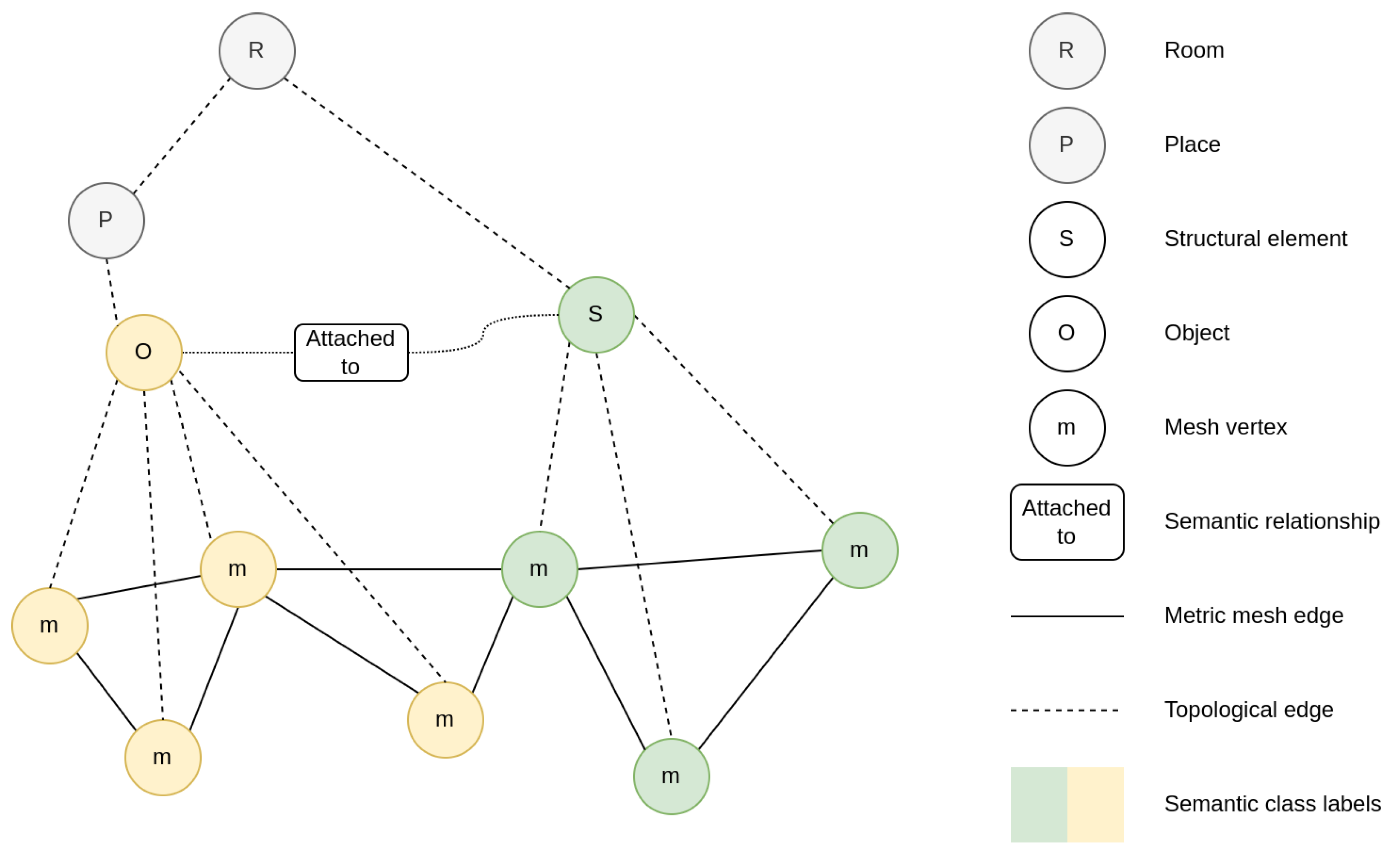
When seeking to abductively reduce a dense, spatial map of a scene into a searchable graph, various fundamentally different definitions of vertices and edges are possible—as exemplified by the control system state and view graphs discussed in [43]—though recently the scene graph [6,7,29], illustrated in Figure 3, has gained considerable notoriety in the space of mapping for robotics, a layered structure with classes of vertices corresponding to entitites, such as spatial points, places in free space, objects, or partitions of space, such as rooms. This builds upon earlier work, such as [53], in implementing the metric–topological–semantic hierarchy of maps, which, in turn, was defined by early research in autonomous robotics [5]. The seamless blending of metric, topological, and semantic information into one map may be compared with attempts to build separate ontology structures, which can perhaps be considered something of a holdover from the knowledge base approach to artificial intelligence which predates the current emphasis on end-to-end machine learning [54,55]. The construction of complex scene graphs from single images is a related problem, which has been studied by the computer vision community—for a more detailed survey of mainly two-dimensional scene graph construction, we direct the reader to [56]. It must be noted, however, that scene graphs are not the only way in which graph structures are used to sparsify spatial maps, a distinctive, domain-specific example being the construction of tree trunk atlases for navigation in a forest environment in lieu of an occupancy map [57,58].
Unlike most of the previously defined concepts, which have a clear mathematical formulation shared by many works, it is difficult to divorce the graph formulations from the construction methods used in each system. Therefore, probably the most concise way to describe them is by giving examples. Specifically, we choose to detail SPIN and SceneGraphFusion.
SPIN (2020) by Rosinol et. al. [6] is a multi-layer mapping framework using Kimera [6] as a base and extended in Hydra [59]. It is capable of placing semantically classified objects in scenes and building place-, structure-, and room-level topological maps.
The Kimera mapping system relies on stereo image and IMU inputs to implement two-stage tracking-mapping keyframe SLAM as discussed in Section 2. Multiple mesh models are constructed at different rates—per-frame and multi-frame local meshes, and a global one which is used in the topology estimation stages. The former two are built by applying a Delaunay triangulation to the image features used in the tracker. The latter, however, is constructed from keyframe stereo range data by first converting this into a TSDF, then applying the marching cubes algorithm. Semantic segmentations of keyframes are back-projected to annotate the mesh.
SPIN then uses this semantically annotated metric map and constructs multiple topological layers on top of it. To be precise, a “layer” in this graph is merely a subset of vertices treated in a specific manner. The lowest layer of this graph is the mesh itself, which is already a graph. The next is that of objects, obtained by either spatially clustering points with a given label, or fitting a 3D model of a known shape when one is available. Each object vertex is then linked with its corresponding vertices in the global mesh and stores attributes, such as a pose and a bounding box. It is also linked to its nearest place vertex. A special case is that of structural members, which are similar to objects but belong to specially designated semantic classes (e.g., ceiling or wall), and are linked to room rather than place vertices. An object may be linked to a structural vertex by a semantically meaningful relation edge (e.g., that of being attached). Agents are much like objects but possess a sequence of poses over time, and observations made of them are masked from the map.
Place vertices, by contrast, are created in regions of free space and linked according to mutual traversability using the ESDF, which was also used to construct the global mesh. Room detection is accomplished by applying a heuristic to horizontal sections of the ESDF, which are assumed to follow the floor plan of a building at a certain height. Room vertices are linked to the place nodes they contain. Among the most salient improvements made by the subsequent Hydra system was doing away with this highly engineered heuristic, and applying morphological operations to the place graph instead. Another major change is the online construction of the global mesh, enabled by a deformation method that enables loop closures to be incorporated after construction.
SceneGraphFusion (2022) by Wu et. al. [7] is notable for the use of GNNs for direct inference on point clouds, enabling the joining of clusters into object instances and adding relations between objects.
A metric surface map is produced from RGB-D data with the method outlined in [35]. However, as each depth image arrives, this is segmented into discrete objects through edge detection-based heuristics and these are then merged into a globally consistent object-level map according to [60]. The output of this process is a set of segments, sets of points associated with discrete objects, from which geometrical properties like centroids and bounding boxes may be estimated.
The scene graph construction method takes this metric map as an input. A pairwise distance heuristic between the segments is used to build a neighbor graph. Uniform vector representations of each segment are produced through the application of a neural network [61] to create latent space embeddings, concatenated with geometric object properties to produce node features. This is reminiscent of the image and text embedding methods discussed in Section 3.3. Each edge in the neighbor graph is associated with an edge feature vector, computed by a multi-layer perceptron (MLP) over the adjacent node features. A GNN is then applied—blending information about each node and its neighbors—for two iterations, in a process known as message passing. Finally, MLPs use this blended information to classify nodes and the semantic relationships between them.
An interesting property of this approach is the fact that semantic information is extracted from the structure of the scene directly, without reliance on image semantic segmentation methods discussed in more detail below. However, it is not hard to see how this message-passing approach could generalize to feature vectors also including, for example, open set labels. Utilizing machine learning to classify edge features in the scene also enables the extraction of more complex inter-object relations than reliance purely on segmented input images.

3.3. Semantics

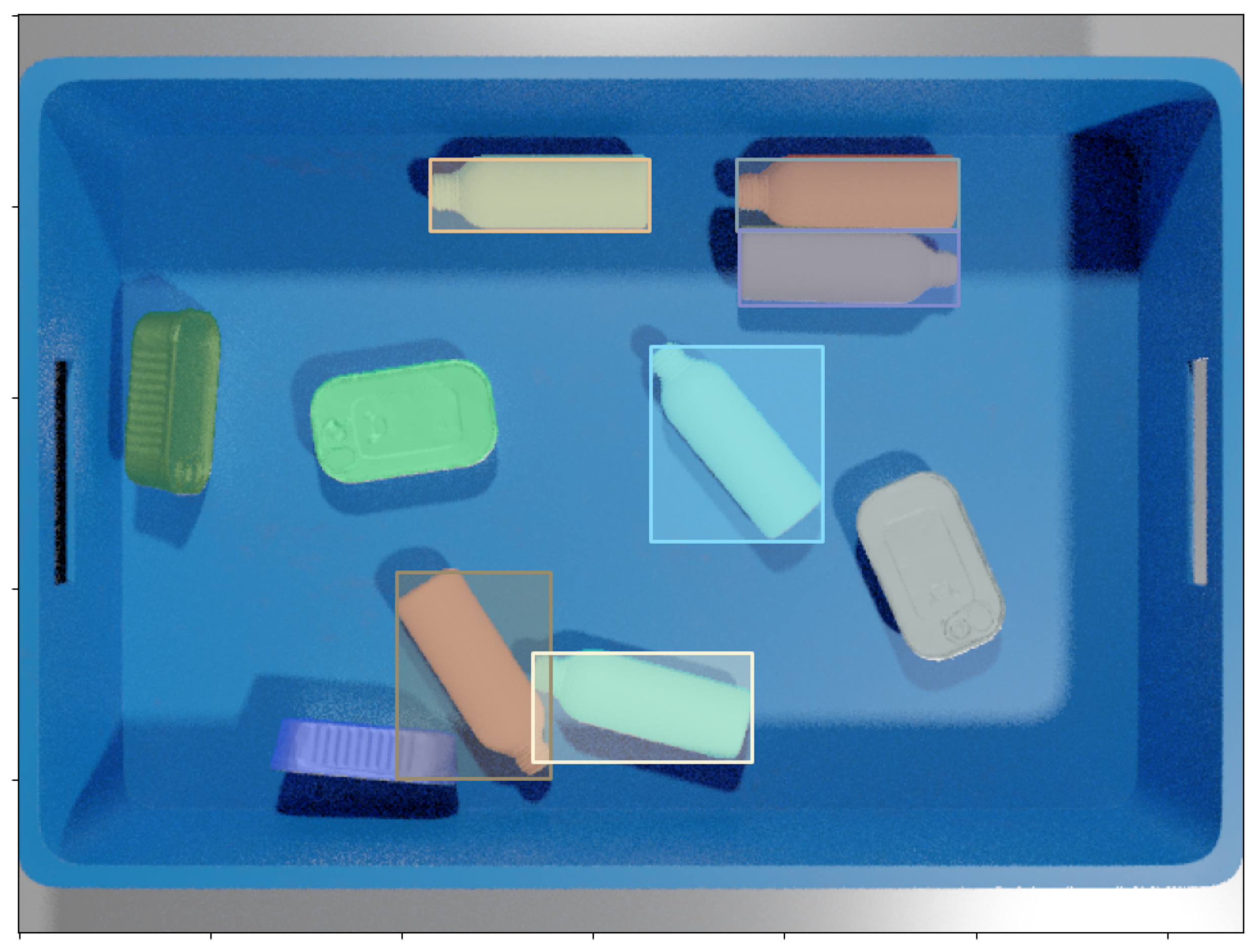
The term semantic map has had various definitions proposed over the decades. Earlier works, in particular, tend to envision a knowledge base-like structure [53,62] where arbitrarily complex, explicit relations between objects and categories of such are possible, and this is still occasionally explored to this day [54,55]. However, realizations of such are hard to come by and systems constrained by real-world implementation concerns tend to limit their object relationships to ones grounded in the spatial configuration of the environment, be they from the dawn of robotic mapping [5] or approaching the current state of the art [7,59]. Indeed, many mapping approaches limit themselves to the discrete object level [45,63,64], while others forgo even that to merely metric map features such as surfels [15,65]. Therefore, in this subsection we give an extremely brief overview of the ways semantics can be inferred from image data, two of which are illustrated in Figure 4, followed by a short exploration of how semantics can be integrated into a map [64].

3.3.1. Object Detection

Object detection involves predicting a semantic class (generally, vector of probabilities), and some type of localization—typically for the pure computer vision task, a rectangular bounding box—for multiple objects in the input data. Some earlier approaches used model-based, hand-engineered heuristic methods to perform 6DoF detection of objects with a known shape in depth image data [63]. However, by the mid-2010s, highly capable neural network-based general-purpose models for object detection in images had become available [66]. While pure object detectors have indeed found use in mapping applications—such as the integration of an object detector to weigh the contributions of multiple EKFs in a filter SLAM system, and produce an object level map [64]—the general trend appears to be that the more fine-grained segmentation methods are preferred.

3.3.2. Image Segmentation—Semantic, Instance, Panoptic

Segmentation is a class of computer vision tasks perhaps best summarized in [67]. Semantic segmentation assigns each pixel in an image one of a set of discrete semantic class labels. Instance segmentation requires that a mask be produced for each object instance in an image, the crucial differences being that one, not the entire image need be covered, and two, the masks corresponding to each instance may overlap. Panoptic segmentation is defined as a middle ground between these two, with pixel-wise class and instance assignments, i.e., covering the entire image with non-overlapping instance segmentation. The background is collated into a “stuff” class as opposed to “things”, objects assigned to one of the distinct semantic classes. The same advances in machine learning that enabled practical object detection models have also produced ones capable of successfully performing these segmentation tasks—indeed, in many cases, these are created by simply augmenting an object detection model with a mask prediction head [68,69], though some were designed with the capability in mind from the ground-up [70]. The various types of segmentation data have been used in various semantic mapping systems, discussed in more detail under map integration.

3.3.3. Open-Set Semantics

To address the inherently limited nature of a finite set of semantic object classes, open-set semantics allow each label to encode arbitrary information about the object. Underlying this direction of research was the invention of text-to-image embeddings, learned in a self-supervised manner by neural network models trained to map images and their captions to similar vectors in a latent space [71]. Turning this image-wide mapping into a pixel-wise segmentation that can be back-projected onto specific points in space has proven quite challenging, but has been successfully accomplished in [15]. Work has also been performed on integrating open-set semantics with implicit scene models [42].

3.3.4. Map Integration

In the case of semantic data inferred from images, some form of back-projection is typically required to turn this into 3D information. For this, the dense pixel-wise segmentation masks are generally more amenable than objects with bounding boxes. Several approaches [15,65] take the dense surfel representation introduced in [14] as a foundation, and blend back-projected annotations into a consistent, semantically annotated map. The previously detailed Kimera also provides a similar capability but projects segmentation data into a TSDF, which is later converted into a mesh. A major additional capability afforded by the provision of semantic information is dynamic masking—enabling moving agents such as humans to be identified and sensory observations related to them to be ignored in map construction. Furthermore, notably with [15], the open-set embeddings that serve as class annotations are vectors, so searches can be performed by producing a text or image embedding and filtering the unstructured point cloud by a metric such as cosine similarity. A different approach is taken in object-level SLAM systems, such as [45,63], which estimate poses at the level of individual objects and integrate them into a PGO problem for improved localization. The main difference is that [63] uses a database of object models as structural priors, whereas [45] uses instance segmentations produced by a neural network model to create a TSDF for each object, associated with a semantic class.
When it comes to higher-order (object relational) semantics, it is clear that pure back-projection of discrete semantic labels is insufficient. The open set annotations introduced by [15] appear to address this somewhat, as they demonstrate ways various queries can be constructed over unordered, vector-annotated point clouds, e.g., finding the distance between objects by specifying object instances through text, finding centroids of the corresponding point clouds, and computing the vector difference. Yet this is far from the knowledge base-like structures envisioned by some earlier works [53,62]. SPIN [6] admits the possibility of inferring such structure in principle, but does not provide an implementation. This leaves GNN-based inference as in [7] as perhaps the most promising in terms of being able to reconstruct complex, arbitrary conceptual maps, yet it does not take advantage of image segmentation.

3.4. Summary

There exist a variety of ways to represent the environment that has been mapped by a robot performing SLAM. At the lowest level, there are metric maps, which conserve the spatial structure of the environment—distances and directions to obstacles—without necessarily providing any other kind of information. Occupancy grid maps (OGMs) are a common type of metric map. Surfel clouds or meshes are more useful when it comes to fine-grained reconstruction of surfaces. Implicit maps, which represent the environment as a continuous function of spatial coordinates, have become a viable alternative to the above with advances in deep learning and neural radiance fields (NRFs).
For path planning and other problems fundamentally based on search algorithms, it is desirable to obtain a graph representation of the environment. This need has been recognized for decades and is typically known as topological mapping. Surface meshes and place graphs are examples of topological map structures. Scene graphs are maps that integrate metric information with multiple layers of topological and semantic graph relationships between points and objects.
Points and graph nodes in a map can be annotated with semantic information, such as object instance and class identifiers. Most commonly, these are obtained through computer vision methods, though directly inferring semantic information from point clouds is also possible. An active area of research is the use of open-set semantic information, where continuous latent space embeddings obtained through neural network encoders replace discrete class labels.

4. Performance Evaluation

As can be seen in the previous sections, a variety of ways exist to tackle every aspect of the map construction problem, and thus consistent benchmarks and evaluation metrics are crucial when trying to assess the viability of different approaches in any given context. The availability of common evaluation data sets is critical, as it is rarely possible for teams working in different locations to test their implementations under the same physical conditions. Some well-known benchmarks include, among others:
  • KITTI [72]—stereo imagery, multi-line LiDAR, IMU tracks, collected over multi-kilometer outdoor tracks in a self-driving vehicle testbed; ground truth poses established with aid of GPS; also includes 3D object instance annotations.
  • RGB-D SLAM benchmark from TUM [73]—RGB-D data of indoor observation sequences collected by custom rig; ground truth data from motion capture equipment; notable for establishing the Absolute Trajectory Error (ATE) metric.
  • EuRoC [74]—a micro aerial vehicle (MAV) stereo, IMU dataset collected indoors; ground truth data established through laser tracking; provides a reference point cloud in some locations.
  • TUM-VI [75]—another stereo-inertial dataset, featuring outdoor sequences, collected with a hand-held rig; ground truth data provided by motion capture equipment, meaning that for longer sequences this is only available at the start and end of the trajectory.
Using these benchmarks, many authors evaluate their systems using the absolute trajectory error (ATE) and relative pose error (RPE) metrics, formalized in [73]. RPE averages the error in relative poses over the entire trajectory—comparing the difference between two subsequent ground truth poses to that between two estimated poses. ATE is an absolute measure, taken by finding a rigid transform to align the ground truth trajectory to the estimate, then averaging the translation between poses at corresponding time steps. While ATE does not directly take orientation into account, [73] notes that due to the effect of rotation estimates on subsequent translations, ATE and RPE values tend to be strongly correlated, but ATE is much more human-readable.
While a systematic comparison of the results attained by various SLAM systems on these benchmarks is outside the scope of this overview, it is informative to note the approximate values one might expect from a modern SLAM system. Table 2 attempts to summarize the extensive comparisons performed in [22] to give the reader a rough, order-of-magnitude estimate of SLAM system accuracy at the time of writing this overview. For this reason, we have only selected systems that have already been discussed above. The variance in results across different trajectories in TUM-VI is too great for meaningful averaging, therefore we have selected long outdoor trajectories for which loop closures are available, in order to demonstrate the drawbacks inherent to tracking-only systems. As can be seen, for short, indoor trajectories, ATE figures on the order of centimeters can be expected. However, drift greatly increases once traversing longer distances outdoors, even when the potential for loop closing exists.
Aside from localization performance, it is also necessary to have ways in which other aspects of a mapping system can be evaluated. At the lowest level, assuming the system outputs a metric map of the environment as a byproduct, and something similar is provided by the evaluation data set, one may simply compute a distance metric between these, as performed, for example, in [29], where the distance between mesh points and the ground truth point cloud provided by [74] is computed after alignment using the iterative closest point algorithm. When working with a more specific problem, such as in [76], where the computer vision aspect of segmenting terrain according to traversability is covered, access to domain-specific datasets becomes very important—in this case with both image-only [77] and 3D point cloud [78] data being available.
Benchmarks in point- and voxel-wise classification, as well as the spatial accuracy of object detection, are provided by datasets such as ScanNet [79]. Higher-order semantics may also be evaluated. For example, [7] evaluate their method against the [80] scene graph dataset, using more involved metrics specifically defined for this purpose such as Recall@K, generalized in [80] from the original 2D image case, which is detailed in [56].

5. Discussion

While by no means exhaustive, the previous sections should give the reader interested in any aspect of the mapping stack a sufficient understanding of the terminology used, as well as an initial set of references, to serve as a starting point for further research. However, we would still like to address some questions that do not necessarily fit into the conceptual explanation.

5.1. Domain-Specific Challenges

In situations that do not approximate typical laboratory conditions very well, one encounters a variety of domain-specific challenges. For example, the aforementioned indoor–outdoor dichotomy in performance is borne out further in studies comparing the performance of different SLAM systems for specific applications, such as agriculture [81]. The authors evaluate a variety of recent SLAM and VIO implementations, among them [17,22,23,25,29], on their ability to provide localization for a weed-removal robot operating in a soybean field. The findings are quite disappointing, as none of the systems attained performance deemed acceptable for the task by the authors, due to issues, such as repetitive appearance, inconsistent scene illumination, and acceleration values that saturate the IMU.
Some ways to overcome the limitations of more traditional mapping approaches have involved looking beyond the typical assortment of sensors available. In [82], a multi-line LiDAR scanner is aligned with a thermal camera, which can often produce much clearer outlines of distinct objects outdoors than a traditional RGB camera, irrespective of external lighting. To this end, they introduce an atypical tracking algorithm that associates spatial points with their projections in adjacent frames by temperature estimates. The use of thermal data complicates loop closure detection, however, as the ambient temperature can vary a great deal over time—something the authors claim to overcome by utilizing an affine illumination model to compensate for these shifts.
Others choose to focus on otherwise constrained problem domains. Several systems designed for use in forestry [57,58] elect to take advantage of what structure they can find—namely, tree trunks. Each uses a different heuristic for tree trunk detection and map representation, but, in both cases, the mapping problem can be significantly simplified by relying on these conveniently naturally occurring landmarks. Furthermore, indeed, the entire field of autonomous driving relies on specialized SLAM systems, often very narrowly fine-tuned for the road environment, to compensate for the imperfect coverage and insufficient precision of extrinsic localization sources, such as satellite-based navigation. This constitutes an extensive field of research in itself, the specifics of which are covered in much more detail than possible here by [83].
It is not just the metric map construction step that is challenging in less structured environments. An obvious application for the integration of semantics into maps could be terrain segmentation according to reversibility, significant for autonomous ground vehicles (AGVs) operating off-road. However, image segmentation by using off-the-shelf models as discussed in Section 3.3 has proven insufficient according to [76], prompting them to introduce their own computer vision model architecture specifically tuned for this part of the mapping stack.

5.2. Robot Navigation without the Construction of Maps

Navigating the environment without deliberately constructing a map is a possibility that arises quite naturally when one ponders how humans accomplish day-to-day tasks without needing detailed occupancy grid maps of their surroundings. Indeed, when looking at recent work using large language models (LLM) to produce complex, high-level plans for mobile manipulators [84], only the most rudimentary map is provided—a set of discrete places the robot can go to. The localization of objects in the robot’s immediate surroundings once there is performed by learned policies conditioned on sensory observations.
It is not hard to imagine that this kind of system could be combined with something like the approaches demonstrated in [2,85]. Given a sequence of navigation instructions in natural language, the former has an LLM to parse out the landmark descriptors, which are compared against sensory observations by a vision-language model (VLM), to produce a topological path through a visual-navigation model (VNM). The latter does away with a map entirely—instead, the robot is controlled directly by a trained policy, which accepts a VLM embedding of the target and a vision model embedding of the current view, along with past actions, as input. However, these kinds of systems are still in their infancy, and do nothing for cases when producing a map of the surroundings might be useful for purposes other than controlling the robot at any given instant.

6. Conclusions

The amount of research performed on map construction clearly indicates that this is deemed a highly important part of the autonomous robot perception, decision-making, and control systems by researchers in the field. The SLAM problem, introduced in Section 2, has reached a considerable degree of maturity with the emergence of a somewhat dominant approach—two-stage tracking-smoothing—over the 2010s indicating that it might be converging towards a well-understood, general-purpose solution, even though a great deal of work remains to be performed, especially as it pertains to maintaining accuracy under challenging outdoor conditions.
By contrast, using the accurate localization data from a SLAM system in conjunction with additional sensor measurements to build higher-level maps, useful beyond merely localizing the robot, appears to be much more of an open problem. With regards to converting points in space into a searchable topology of places, at least, the scene graph may well prove the way forward. However, the knowledge-base style abstract semantic layers as envisioned by early proponents of multi-level mapping do not yet show much evidence of practical use. While off-the-shelf solutions for obtaining semantic information—such as image segmentation models—have been widely used to annotate spatial locations with discrete or continuous labels, these do not necessarily generalize well to some problems that may be of great interest to robotics researchers—such as segmenting terrain according to traversability—leaving room for domain-specific finetuning.

Author Contributions

Conceptualization, P.R. and J.A.; investigation, P.R.; writing—original draft preparation, P.R.; writing—review and editing, P.R., J.A. and M.G.; visualization, P.R.; supervision, J.A.; project administration, M.G.; funding acquisition, J.A. and M.G. All authors have read and agreed to the published version of the manuscript.

Funding

This research is funded by the Latvian Council of Science, project “Smart Materials, Photonics, Technologies and Engineering Ecosystem” No. VPP-EM-FOTONIKA-2022/1-0001.

Data Availability Statement

Data sharing not applicable.

Conflicts of Interest

The authors declare no conflict of interest.

References

  1. Arents, J.; Greitans, M. Smart Industrial Robot Control Trends, Challenges and Opportunities within Manufacturing. Appl. Sci. 2022, 12, 937. [Google Scholar] [CrossRef]
  2. Majumdar, A.; Aggarwal, G.; Devnani, B.; Hoffman, J.; Batra, D. ZSON: Zero-Shot Object-Goal Navigation using Multimodal Goal Embeddings. arXiv 2022, arXiv:2206.12403. [Google Scholar]
  3. ROS Wiki: Movebase Global Planner. Available online: https://wiki.ros.org/global_planner (accessed on 29 June 2023).
  4. Kuipers, B. Modeling Spatial Knowledge. Cogn. Sci. 1978, 2, 129–153. [Google Scholar] [CrossRef]
  5. Chatila, R.; Laumond, J.P. Position referencing and consistent world modeling for mobile robots. In Proceedings 1985 IEEE International Conference on Robotics and Automation; IEEE: Piscataway, NJ, USA, 1985; Volume 2, pp. 138–145. [Google Scholar]
  6. Rosinol, A.; Gupta, A.; Abate, M.; Shi, J.; Carlone, L. 3D Dynamic Scene Graphs: Actionable Spatial Perception with Places, Objects, and Humans. arXiv 2020, arXiv:2002.06289. [Google Scholar]
  7. Cheng, W.S.; Wald, J.; Tateno, K.; Navab, N.; Tombari, F. SceneGraphFusion: Incremental 3D Scene Graph Prediction from RGB-D Sequences. In Proceedings of the 2021 IEEE/CVF Conference on Computer Vision and Pattern Recognition (CVPR), Nashville, TN, USA, 20–25 June 2021; pp. 7511–7521. [Google Scholar]
  8. Thrun, S.; Burgard, W.; Fox, D. Probabilistic Robotics; MIT Press: Cambridge, MA, USA, 2005. [Google Scholar]
  9. Dellaert, F.; Kaess, M. Factor Graphs for Robot Perception. Found. Trends Robot. 2017, 6, 1–139. [Google Scholar] [CrossRef]
  10. Alkendi, Y.; Seneviratne, L.; Zweiri, Y. State of the Art in Vision-Based Localization Techniques for Autonomous Navigation Systems. IEEE Access 2021, 9, 76847–76874. [Google Scholar] [CrossRef]
  11. Huang, B.; Zhao, J.; Liu, J. A Survey of Simultaneous Localization and Mapping. arXiv 2019, arXiv:1909.05214. [Google Scholar]
  12. Garg, S.; Sunderhauf, N.; Dayoub, F.; Morrison, D.; Cosgun, A.; Carneiro, G.; Wu, Q.; Chin, T.J.; Reid, I.D.; Gould, S.; et al. Semantics for Robotic Mapping, Perception and Interaction: A Survey. arXiv 2021, arXiv:2101.00443. [Google Scholar]
  13. Osman, H.; Darwish, N.; Bayoumi, A. PlaceNet: A multi-scale semantic-aware model for visual loop closure detection. Eng. Appl. Artif. Intell. 2023, 119, 105797. [Google Scholar] [CrossRef]
  14. Newcombe, R.A.; Davison, A.J. Live dense reconstruction with a single moving camera. In Proceedings of the 2010 IEEE Computer Society Conference on Computer Vision and Pattern Recognition, San Francisco, CA, USA, 13–18 June 2010; pp. 1498–1505. [Google Scholar]
  15. Jatavallabhula, K.M.; Kuwajerwala, A.; Gu, Q.; Omama, M.; Chen, T.; Li, S.; Iyer, G.; Saryazdi, S.; Keetha, N.V.; Tewari, A.K.; et al. ConceptFusion: Open-set Multimodal 3D Mapping. arXiv 2023, arXiv:2302.07241. [Google Scholar]
  16. Lu, G.; Yang, H.; Li, J.; Kuang, Z.; Yang, R. A Lightweight Real-Time 3D LiDAR SLAM for Autonomous Vehicles in Large-Scale Urban Environment. IEEE Access 2023, 11, 12594–12606. [Google Scholar] [CrossRef]
  17. Bloesch, M.; Omari, S.; Hutter, M.; Siegwart, R. Robust visual inertial odometry using a direct EKF-based approach. In Proceedings of the 2015 IEEE/RSJ International Conference on Intelligent Robots and Systems (IROS), Hamburg, Germany, 28 September–2 October 2015; pp. 298–304. [Google Scholar] [CrossRef] [Green Version]
  18. Yang, N.; Stumberg, L.v.; Wang, R.; Cremers, D. D3VO: Deep Depth, Deep Pose and Deep Uncertainty for Monocular Visual Odometry. In Proceedings of the IEEE/CVF Conference on Computer Vision and Pattern Recognition (CVPR), Seattle, WA, USA, 13–19 June 2020. [Google Scholar]
  19. Xu, W.; Cai, Y.; He, D.; Lin, J.; Zhang, F. FAST-LIO2: Fast Direct LiDAR-Inertial Odometry. IEEE Trans. Robot. 2022, 38, 2053–2073. [Google Scholar] [CrossRef]
  20. Leutenegger, S.; Furgale, P.T.; Rabaud, V.; Chli, M.; Konolige, K.; Siegwart, R.Y. Keyframe-Based Visual-Inertial SLAM using Nonlinear Optimization. In Proceedings of the Robotics: Science and Systems, Berlin, Germany, 24–28 June 2013. [Google Scholar]
  21. Mur-Artal, R.; Montiel, J.M.M.; Tardós, J.D. ORB-SLAM: A Versatile and Accurate Monocular SLAM System. IEEE Trans. Robot. 2015, 31, 1147–1163. [Google Scholar] [CrossRef] [Green Version]
  22. Campos, C.; Elvira, R.; Rodr’iguez, J.J.G.; Montiel, J.M.M.; Tardós, J.D. ORB-SLAM3: An Accurate Open-Source Library for Visual, Visual–Inertial, and Multimap SLAM. IEEE Trans. Robot. 2020, 37, 1874–1890. [Google Scholar] [CrossRef]
  23. Qin, T.; Li, P.; Shen, S. VINS-Mono: A Robust and Versatile Monocular Visual-Inertial State Estimator. IEEE Trans. Robot. 2018, 34, 1004–1020. [Google Scholar] [CrossRef] [Green Version]
  24. Hartley, R.; Zisserman, A. Multiple View Geometry in Computer Vision, 2nd ed.; Cambridge University Press: Cambridge, MA, USA, 2004. [Google Scholar] [CrossRef] [Green Version]
  25. Sun, K.; Mohta, K.; Pfrommer, B.; Watterson, M.; Liu, S.; Mulgaonkar, Y.; Taylor, C.J.; Kumar, V. Robust Stereo Visual Inertial Odometry for Fast Autonomous Flight. IEEE Robot. Autom. Lett. 2018, 3, 965–972. [Google Scholar] [CrossRef] [Green Version]
  26. Frey, B.J.; Kschischang, F.R.; Loeliger, H.A.; Wiberg, N. Factor graphs and algorithms. In Proceedings of the Annual Allerton Conference on Communication Control and Computing, Citeseer, Cambridge, UK, 29 September–1 October 1997; Volume 35, pp. 666–680. [Google Scholar]
  27. Fourie, D.; Leonard, J.; Kaess, M. A nonparametric belief solution to the Bayes tree. In Proceedings of the 2016 IEEE/RSJ International Conference on Intelligent Robots and Systems (IROS), Daejeon, Republic of Korea, 9–14 October 2016; pp. 2189–2196. [Google Scholar] [CrossRef] [Green Version]
  28. Dellaert, F.; Contributors. Borglab/Gtsam. Available online: https://zenodo.org/record/7582634 (accessed on 29 June 2023).
  29. Rosinol, A.; Abate, M.; Chang, Y.; Carlone, L. Kimera: An Open-Source Library for Real-Time Metric-Semantic Localization and Mapping. In Proceedings of the 2020 IEEE International Conference on Robotics and Automation (ICRA), Paris, France, 31 May–31 August 2020; pp. 1689–1696. [Google Scholar] [CrossRef]
  30. Gálvez-López, D.; Tardós, J.D. Bags of Binary Words for Fast Place Recognition in Image Sequences. IEEE Trans. Robot. 2012, 28, 1188–1197. [Google Scholar] [CrossRef]
  31. Dellaert, F. Factor Graphs: Exploiting Structure in Robotics. Annu. Rev. Control. Robot. Auton. Syst. 2021, 4, 141–166. [Google Scholar] [CrossRef]
  32. Forster, C.; Carlone, L.; Dellaert, F.; Scaramuzza, D. IMU Preintegration on Manifold for Efficient Visual-Inertial Maximum-a-Posteriori Estimation. In Proceedings of the Robotics: Science and Systems, Rome, Italy, 13–17 July 2015. [Google Scholar]
  33. Hess, W.; Kohler, D.; Rapp, H.; Andor, D. Real-time loop closure in 2D LIDAR SLAM. In Proceedings of the 2016 IEEE International Conference on Robotics and Automation (ICRA), Stockholm, Sweden, 16–21 May 2016; pp. 1271–1278. [Google Scholar] [CrossRef]
  34. Schneider, T.; Dymczyk, M.; Fehr, M.; Egger, K.; Lynen, S.; Gilitschenski, I.; Siegwart, R. Maplab: An Open Framework for Research in Visual-Inertial Mapping and Localization. IEEE Robot. Autom. Lett. 2018, 3, 1418–1425. [Google Scholar] [CrossRef] [Green Version]
  35. Keller, M.; Lefloch, D.; Lambers, M.; Izadi, S.; Weyrich, T.; Kolb, A. Real-Time 3D Reconstruction in Dynamic Scenes Using Point-Based Fusion. In Proceedings of the 2013 International Conference on 3D Vision, Seattle, WA, USA, 29 June–1 July 2013; pp. 1–8. [Google Scholar]
  36. Whelan, T.; Salas-Moreno, R.F.; Glocker, B.; Davison, A.J.; Leutenegger, S. ElasticFusion: Real-time dense SLAM and light source estimation. Int. J. Robot. Res. 2016, 35, 1697–1716. [Google Scholar] [CrossRef] [Green Version]
  37. Sucar, E.; Liu, S.; Ortiz, J.; Davison, A.J. iMAP: Implicit Mapping and Positioning in Real-Time. In Proceedings of the 2021 IEEE/CVF International Conference on Computer Vision (ICCV), Montreal, QC, Canada, 10–17 October 2021; pp. 6209–6218. [Google Scholar] [CrossRef]
  38. Klein, G.S.W.; Murray, D.W. Parallel Tracking and Mapping for Small AR Workspaces. In Proceedings of the 2007 6th IEEE and ACM International Symposium on Mixed and Augmented Reality, Nara, Japan, 13–16 November 2007; pp. 225–234. [Google Scholar]
  39. Rublee, E.; Rabaud, V.; Konolige, K.; Bradski, G.R. ORB: An efficient alternative to SIFT or SURF. In Proceedings of the 2011 International Conference on Computer Vision, Barcelona, Spain, 6–12 November 2011; pp. 2564–2571. [Google Scholar]
  40. Kaess, M.; Johannsson, H.; Roberts, R.; Ila, V.; Leonard, J.J.; Dellaert, F. iSAM2: Incremental smoothing and mapping using the Bayes tree. Int. J. Robot. Res. 2012, 31, 216–235. [Google Scholar] [CrossRef]
  41. Mildenhall, B.; Srinivasan, P.P.; Tancik, M.; Barron, J.T.; Ramamoorthi, R.; Ng, R. NeRF: Representing Scenes as Neural Radiance Fields for View Synthesis. arXiv 2020, arXiv:2003.08934. [Google Scholar] [CrossRef]
  42. Mazur, K.; Sucar, E.; Davison, A.J. Feature-Realistic Neural Fusion for Real-Time, Open Set Scene Understanding. arXiv 2022, arXiv:2210.03043. [Google Scholar]
  43. Kuipers, B. The Spatial Semantic Hierarchy. Artif. Intell. 2000, 119, 191–233. [Google Scholar] [CrossRef] [Green Version]
  44. Lavalle, S.M. Planning Algorithms; Cambridge University Press: Cambridge, UK, 2006. [Google Scholar]
  45. Mccormac, J.; Clark, R.; Bloesch, M.; Davison, A.; Leutenegger, S. Fusion++: Volumetric Object-Level SLAM. In Proceedings of the 2018 International Conference on 3D Vision (3DV), Verona, Italy, 5–8 September 2018; pp. 32–41. [Google Scholar]
  46. Crespo, J.; Castillo, J.C.; Mozos, O.M.; Barber, R. Semantic Information for Robot Navigation: A Survey. Appl. Sci. 2020, 10, 497. [Google Scholar] [CrossRef] [Green Version]
  47. Han, X.; Li, S.; Wang, X.; Zhou, W. Semantic Mapping for Mobile Robots in Indoor Scenes: A Survey. Information 2021, 12, 92. [Google Scholar] [CrossRef]
  48. Newcombe, R.A.; Lovegrove, S.J.; Davison, A.J. DTAM: Dense tracking and mapping in real-time. In Proceedings of the 2011 International Conference on Computer Vision, Barcelona, Spain, 6–13 November 2011; pp. 2320–2327. [Google Scholar] [CrossRef] [Green Version]
  49. Curless, B.; Levoy, M. A volumetric method for building complex models from range images. In Proceedings of the 23rd Annual Conference on Computer Graphics and Interactive Techniques, New Orleans, LA, USA, 4–9 August 1996. [Google Scholar]
  50. Zeng, M.; Zhao, F.; Zheng, J.; Liu, X. Octree-based fusion for realtime 3D reconstruction. Graph. Model. 2013, 75, 126–136. [Google Scholar] [CrossRef]
  51. Siddiqui, Y.; Porzi, L.; Bul’o, S.R.; Muller, N.; Nießner, M.; Dai, A.; Kontschieder, P. Panoptic Lifting for 3D Scene Understanding with Neural Fields. arXiv 2022, arXiv:2212.09802. [Google Scholar]
  52. Shafiullah, N.M.M.; Paxton, C.; Pinto, L.; Chintala, S.; Szlam, A.D. CLIP-Fields: Weakly Supervised Semantic Fields for Robotic Memory. arXiv 2022, arXiv:2210.05663. [Google Scholar]
  53. Zender, H.; Mozos, Ó.M.; Jensfelt, P.; Kruijff, G.J.M.; Burgard, W. Conceptual spatial representations for indoor mobile robots. Robot. Auton. Syst. 2008, 56, 493–502. [Google Scholar] [CrossRef] [Green Version]
  54. Chang, D.S.; Cho, G.H.; Choi, Y.S. Ontology-based knowledge model for human–robot interactive services. In Proceedings of the 35th Annual ACM Symposium on Applied Computing, Brno, Czech Republic, 30 March–3 April 2020. [Google Scholar]
  55. Sun, X.; Zhang, Y.; Chen, J. High-Level Smart Decision Making of a Robot Based on Ontology in a Search and Rescue Scenario. Future Internet 2019, 11, 230. [Google Scholar] [CrossRef] [Green Version]
  56. Zhu, G.; Zhang, L.; Jiang, Y.; Dang, Y.; Hou, H.; Shen, P.; Feng, M.; Zhao, X.; Miao, Q.; Shah, S.A.A.; et al. Scene Graph Generation: A Comprehensive Survey. arXiv 2022, arXiv:2201.00443. [Google Scholar]
  57. Li, Q.; Nevalainen, P.; Peña Queralta, J.; Heikkonen, J.; Westerlund, T. Localization in Unstructured Environments: Towards Autonomous Robots in Forests with Delaunay Triangulation. Remote Sens. 2020, 12, 1870. [Google Scholar] [CrossRef]
  58. Nie, F.; Zhang, W.; Wang, Y.; Shi, Y.; Huang, Q. A Forest 3-D Lidar SLAM System for Rubber-Tapping Robot Based on Trunk Center Atlas. IEEE/ASME Trans. Mechatronics 2022, 27, 2623–2633. [Google Scholar] [CrossRef]
  59. Hughes, N.; Chang, Y.; Carlone, L. Hydra: A Real-time Spatial Perception System for 3D Scene Graph Construction and Optimization. In Proceedings of the Robotics: Science and Systems XVIII, New York, NY, USA, 27 June–1 July 2022. [Google Scholar]
  60. Tateno, K.; Tombari, F.; Navab, N. Real-time and scalable incremental segmentation on dense SLAM. In Proceedings of the 2015 IEEE/RSJ International Conference on Intelligent Robots and Systems (IROS), Hamburg, Germany, 28 September–2 October 2015; pp. 4465–4472. [Google Scholar]
  61. Qi, C.; Su, H.; Mo, K.; Guibas, L.J. PointNet: Deep Learning on Point Sets for 3D Classification and Segmentation. In Proceedings of the 2017 IEEE Conference on Computer Vision and Pattern Recognition (CVPR), Honolulu, HI, USA, 21–26 July 2017; pp. 77–85. [Google Scholar]
  62. Galindo, C.; Saffiotti, A.; Coradeschi, S.; Buschka, P.; Fernandez-Madrigal, J.; Gonzalez, J. Multi-hierarchical semantic maps for mobile robotics. In Proceedings of the 2005 IEEE/RSJ International Conference on Intelligent Robots and Systems, Edmonton, AL, Canada, 2–6 August 2005; pp. 2278–2283. [Google Scholar] [CrossRef]
  63. Salas-Moreno, R.F.; Newcombe, R.A.; Strasdat, H.; Kelly, P.H.; Davison, A.J. SLAM++: Simultaneous Localisation and Mapping at the Level of Objects. In Proceedings of the 2013 IEEE Conference on Computer Vision and Pattern Recognition, Portland, OR, USA, 23–28 June 2013; pp. 1352–1359. [Google Scholar] [CrossRef] [Green Version]
  64. Dong, J.; Fei, X.; Soatto, S. Visual-Inertial-Semantic Scene Representation for 3D Object Detection. In Proceedings of the 2017 IEEE Conference on Computer Vision and Pattern Recognition (CVPR), Honolulu, Hawaii, USA, 21–26 July 2017; pp. 3567–3577. [Google Scholar] [CrossRef] [Green Version]
  65. McCormac, J.; Handa, A.; Davison, A.; Leutenegger, S. SemanticFusion: Dense 3D semantic mapping with convolutional neural networks. In Proceedings of the 2017 IEEE International Conference on Robotics and Automation (ICRA), Singapore, 29 May–3 June 2017; pp. 4628–4635. [Google Scholar] [CrossRef] [Green Version]
  66. Redmon, J.; Divvala, S.K.; Girshick, R.B.; Farhadi, A. You Only Look Once: Unified, Real-Time Object Detection. In Proceedings of the 2016 IEEE Conference on Computer Vision and Pattern Recognition (CVPR), Las Vegas, NV, USA, 26 June–1 July 2016; pp. 779–788. [Google Scholar]
  67. Kirillov, A.; He, K.; Girshick, R.B.; Rother, C.; Dollár, P. Panoptic Segmentation. In Proceedings of the 2019 IEEE/CVF Conference on Computer Vision and Pattern Recognition (CVPR), Long Beach, CA, USA, 15–20 June; pp. 9396–9405.
  68. He, K.; Gkioxari, G.; Dollár, P.; Girshick, R.B. Mask R-CNN. IEEE Trans. Pattern Anal. Mach. Intell. 2017, 42, 386–397. [Google Scholar] [CrossRef]
  69. Carion, N.; Massa, F.; Synnaeve, G.; Usunier, N.; Kirillov, A.; Zagoruyko, S. End-to-End Object Detection with Transformers. arXiv 2020, arXiv:2005.12872. [Google Scholar]
  70. Wang, X.; Kong, T.; Shen, C.; Jiang, Y.; Li, L. SOLO: Segmenting Objects by Locations. arXiv 2019, arXiv:1912.04488. [Google Scholar]
  71. Radford, A.; Kim, J.W.; Hallacy, C.; Ramesh, A.; Goh, G.; Agarwal, S.; Sastry, G.; Askell, A.; Mishkin, P.; Clark, J.; et al. Learning Transferable Visual Models From Natural Language Supervision. In Proceedings of the International Conference on Machine Learning, Virtual, 18–24 July 2021. [Google Scholar]
  72. Geiger, A.; Lenz, P.; Urtasun, R. Are we ready for autonomous driving? The KITTI vision benchmark suite. In Proceedings of the 2012 IEEE Conference on Computer Vision and Pattern Recognition, Providence, RI, USA, 16–21 June 2012; pp. 3354–3361. [Google Scholar]
  73. Sturm, J.; Engelhard, N.; Endres, F.; Burgard, W.; Cremers, D. A benchmark for the evaluation of RGB-D SLAM systems. In Proceedings of the IEEE/RSJ International Conference on Intelligent Robots and Systems, Vancouver, BC, Canada, 24–28 September 2012; pp. 573–580. [Google Scholar]
  74. Burri, M.; Nikolic, J.; Gohl, P.; Schneider, T.; Rehder, J.; Omari, S.; Achtelik, M.W.; Siegwart, R. The EuRoC micro aerial vehicle datasets. Int. J. Robot. Res. 2016, 35, 1157–1163. [Google Scholar] [CrossRef]
  75. Schubert, D.; Goll, T.; Demmel, N.; Usenko, V.C.; Stückler, J.; Cremers, D. The TUM VI Benchmark for Evaluating Visual-Inertial Odometry. In Proceedings of the 2018 IEEE/RSJ International Conference on Intelligent Robots and Systems (IROS), Kyoto, Japan, 23–27 October 2018; pp. 1680–1687. [Google Scholar]
  76. Guan, T.; Kothandaraman, D.; Chandra, R.; Manocha, D. GANav: Group-wise Attention Network for Classifying Navigable Regions in Unstructured Outdoor Environments. arXiv 2021, arXiv:2103.04233. [Google Scholar]
  77. Wigness, M.; Eum, S.; Rogers, J.G.; Han, D.; Kwon, H. A RUGD Dataset for Autonomous Navigation and Visual Perception in Unstructured Outdoor Environments. In Proceedings of the International Conference on Intelligent Robots and Systems (IROS), The Venetian Macao, Macau, 3–8 November 2019. [Google Scholar]
  78. Jiang, P.; Osteen, P.R.; Wigness, M.B.; Saripalli, S. RELLIS-3D Dataset: Data, Benchmarks and Analysis. In Proceedings of the 2021 IEEE International Conference on Robotics and Automation (ICRA), Xi’an, China, 30 May–5 June; pp. 1110–1116.
  79. Dai, A.; Chang, A.X.; Savva, M.; Halber, M.; Funkhouser, T.A.; Nießner, M. ScanNet: Richly-Annotated 3D Reconstructions of Indoor Scenes. In Proceedings of the 2017 IEEE Conference on Computer Vision and Pattern Recognition (CVPR), Honolulu, HI, USA, 21–26 July 2017; pp. 2432–2443. [Google Scholar]
  80. Wald, J.; Dhamo, H.; Navab, N.; Tombari, F. Learning 3D Semantic Scene Graphs From 3D Indoor Reconstructions. In Proceedings of the 2020 IEEE/CVF Conference on Computer Vision and Pattern Recognition (CVPR), Seattle, WA, USA, 13–19 June 2020; pp. 3960–3969. [Google Scholar]
  81. Cremona, J.; Comelli, R.; Pire, T. Experimental evaluation of Visual-Inertial Odometry systems for arable farming. J. Field Robot. 2022, 39, 1123–1137. [Google Scholar] [CrossRef]
  82. Shin, Y.S.; Kim, A. Sparse Depth Enhanced Direct Thermal-Infrared SLAM Beyond the Visible Spectrum. IEEE Robot. Autom. Lett. 2019, 4, 2918–2925. [Google Scholar] [CrossRef] [Green Version]
  83. Badue, C.S.; Guidolini, R.; Carneiro, R.V.; Azevedo, P.; Cardoso, V.B.; Forechi, A.; Jesus, L.F.R.; Berriel, R.; Paixão, T.M.; Mutz, F.W.; et al. Self-Driving Cars: A Survey. arXiv 2019, arXiv:1901.04407. [Google Scholar] [CrossRef]
  84. Ahn, M.; Brohan, A.; Brown, N.; Chebotar, Y.; Cortes, O.; David, B.; Finn, C.; Gopalakrishnan, K.; Hausman, K.; Herzog, A.; et al. Do As I Can, Not As I Say: Grounding Language in Robotic Affordances. In Proceedings of the Conference on Robot Learning, Auckland, New Zealand, 14–18 December 2022. [Google Scholar]
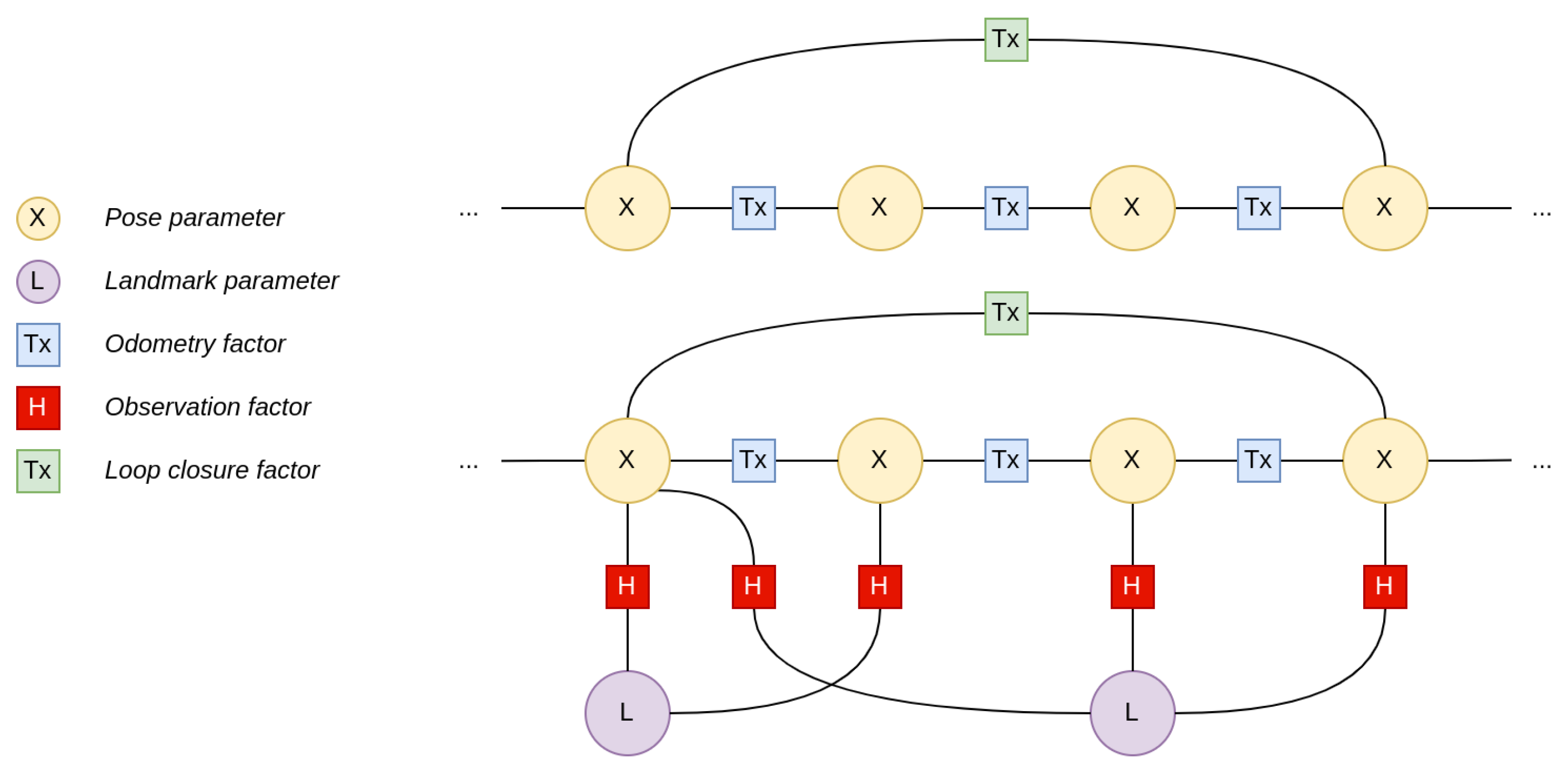
  85. Shah, D.; Osinski, B.; Ichter, B.; Levine, S. LM-Nav: Robotic Navigation with Large Pre-Trained Models of Language, Vision, and Action. In Proceedings of the Conference on Robot Learning, Auckland, New Zealand, 14–18 December 2022. [Google Scholar]
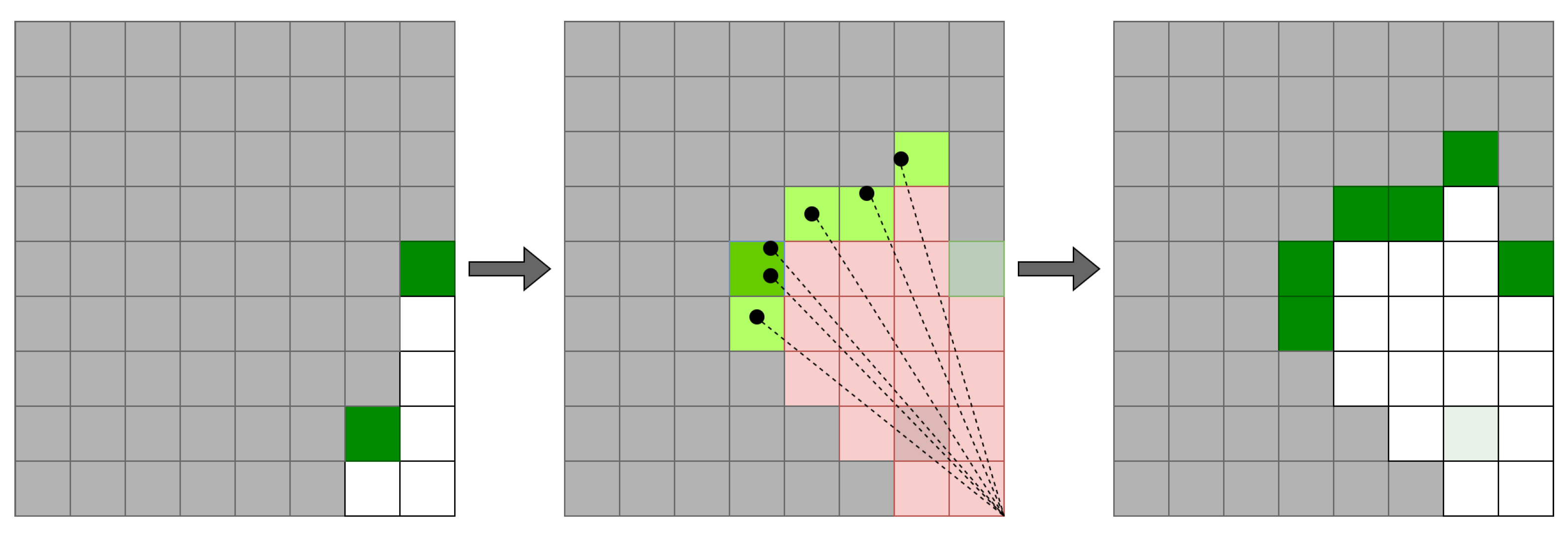
Figure 1. Example factor graph configurations for a pose graph optimization (top) and landmark SLAM (bottom) problem, respectively.
Electronics 12 02925 g001
Figure 2. An occupancy grid map with a realistic update heuristic, as described in [33]. Green indicates a high occupancy score, white — the obverse. Grey cells are uninitialized. A log-odds update increases or decreases the estimated probabilities of a grid square being occupied when a scan point (black dot) is located within it or beyond it (dashed line) respectively. Untouched squares are not affected, and uninitialized values are unknown.
Electronics 12 02925 g002
Figure 3. Example of a scene graph structure like the one described in [6].
Electronics 12 02925 g003
Figure 4. Ground truth data used to train a joint object detection and instance segmentation model. Each bottle and can in the image is assigned an instance mask—shown in different colors—and the bottles also have bounding boxes.
Electronics 12 02925 g004
Table 1. Comparison of selected mapping systems by SLAM implementation.
SystemSensors 1Tracking 2Smoothing 3Note
ORB-SLAM (2017) [21]VTwo-stage local BAFrame descriptors for loop detection, PGO
ORB-SLAM3 (2020) [22]V, VI, S, SITwo-stage local BA with optional IMU, stereo factorsFrame descriptors for loop detection, multiple maps, PGOExtension of [21]
Google Cartographer (2016) [33]2L, 3LScan pose optimization with regard to local OGMGeometric feature-based loop detection between local OGMs, PGO
Maplab (2017) [34]VIROVIO [17] EKFOptimization performed offline through external tools
Keller et al. (2013) [35]DICP with regard to a fixed surfel modelNone for camera poses; Depth point averagingBasis for many other systems, e.g., [7,15,36]
iMap (2021) [37]DCamera pose optimization with regard to NRF with frozen weightsJoint camera pose and NRF optimization
1 V—monocular visual; VI—visual-inertial; S(SI)—stereo(-inertial); D(DI)–RGB-D(-inertial); 2L–2D (1-line) LiDAR; 3L–3D (multi-line) LiDAR; 2 BA—bundle adjustment; EKF—extended Kalman filter; OGM—occupancy grid map; 3 PGO—pose graph optimization.
Table 2. Illustrative performance baselines by benchmark, per [22].
SystemBenchmarkScore
ORB-SLAM (2017) [21]EuRoC V 3, ATE0.047 1
ORB-SLAM3 (2020) [22]0.041 1
ORB-SLAM3 (2020) [22]EuRoC VI 3, ATE0.043
ROVIO (2015) 2 [17]0.224
ORB-SLAM3 (2020) [22]EuRoC SI 3, ATE0.035
Kimera (2020) [29]0.119
ORB-SLAM3 (2020) [22]TUM-VI outdoors5 4,5, ATE8.95
ROVIO (2015) 2 [17]54.32
ORB-SLAM3 (2020) [22]TUM-VI outdoors7 4,6, ATE4.58
ROVIO (2015) 2 [17]49.01
1 Did not complete all trajectories; 2 EKF approach used in Maplab [34], for tracking-only comparison; 3 V—visual; VI—visual-inertial; SI—stereo-inertial; 4 outdoors5, outdoors7 selected due to availability of loop-closure constraints; 5 path length 1168 m; 6 path length 1748 m.
Disclaimer/Publisher’s Note: The statements, opinions and data contained in all publications are solely those of the individual author(s) and contributor(s) and not of MDPI and/or the editor(s). MDPI and/or the editor(s) disclaim responsibility for any injury to people or property resulting from any ideas, methods, instructions or products referred to in the content.