UGV Coverage Path Planning: An Energy-Efficient Approach through Turn Reduction

Abstract

With the advent and rapid growth of automation, unmanned ground vehicles (UGVs) have emerged as a crucial technology, with applications spanning various domains, from agriculture to surveillance, logistics, and military operations. Alongside this surge in the utilization of robotics, novel complications inevitably emerge, posing intriguing questions and challenges to the academic and technological sectors. One such pressing challenge is the coverage path planning (CPP) problem, particularly the notion of optimizing UGV energy utilization during path planning, a significant yet relatively unexplored aspect within the research landscape. While numerous studies have proposed solutions to CPP with a single UGV, the introduction of multiple UGVs within a single environment reveals a unique set of challenges. A paramount concern in multi-UGV CPP is the effective allocation and division of the area among the UGVs. To address this issue, we propose an innovative approach that first segments the area into multiple subareas, which are then allocated to individual UGVs. Our methodology employs fine-tuned spanning trees to minimize the number of turns during navigation, resulting in more efficient and energy-aware coverage paths. As opposed to existing research focusing on models that allocate without optimization, our model utilizes a terrain-aware cost function, and an adaptive path replanning module, leading to a more flexible, effective, and energy-efficient path-planning solution. A series of simulations demonstrated the robustness and efficacy of our approach, highlighting its potential to significantly improve UGV endurance and mission effectiveness, even in challenging terrain conditions. The proposed solution provides a substantial contribution to the field of UGV path planning, addressing a crucial gap and enhancing the body of knowledge surrounding energy-efficient CPP for multi-UGV scenarios.

1. Introduction

The profound impacts of technology and scientific advancements on society are indisputable, transforming the ways we live, work, and interact. Over the last few decades, these breakthroughs have fueled the emergence of an automated society, with robotics taking center stage [1,2]. The adoption and application of robotics and automation systems have skyrocketed, permeating every facet of life, from manufacturing and logistics [3] to agriculture [4,5] and healthcare [6]. In essence, these technological innovations have redefined the concept of work, replacing traditional, manual, and often laborious tasks with automated, efficient, and precise robotic operations.

One of the fundamental components of robotics, directly contributing to its efficacy and utility, is the concept of navigation, specifically, coverage path planning (CPP) [7,8,9]. In simple terms, CPP refers to the task of devising a path for a robot to cover an entire accessible area within a predetermined environment. This technology underpins several applications, including field surveillance, environmental monitoring, and precision agriculture, among others. Achieving optimal CPP is critical as it enables effective area coverage, reduces operational time, and minimizes energy consumption. However, this task becomes more complicated in multi-robot situations. Multi-robot CPP involves not only finding optimal paths for individual robots (such as UAVs [10], UGVs [11], and hybrid robots [12]) but also effective allocation and division of the area among multiple robots [13]. These considerations are critical to avoid duplication of work, prevent robot collisions, and ensure a balanced workload among the robots, contributing to the overall operational efficiency and effectiveness.

In the realm of CPP and robot navigation in general, two major classes of algorithms are prevalent: online and offline. Offline algorithms necessitate comprehensive knowledge of the environment prior to operation commencement, involving the precomputation of a global plan. They are particularly suited to static environments where the layout and obstacles remain unchanged. This paradigm is particularly suitable for agricultural applications, patrolling vehicles, etc. [4,5]. Conversely, online algorithms allow for real-time decision making based on sensor inputs, without the requirement of total environmental understanding prior to deployment. These are adapted for dynamic environments replete with uncertainty, offering quick responses to environmental changes [14,15,16]. Even though these algorithms can typically adapt to the dynamic constraints of the environment, such as moving obstacles, they may lack the comprehensive perspective provided by offline planning and can often lead to suboptimal global solutions.

The scientific community has devoted considerable effort to addressing the offline multi-UGV CPP problem, with several intriguing strategies and methodologies emerging over the years [8,9,10,11,12,13,17,18,19,20,21,22]. A fundamental insight that underpins many of these methodologies is that the multi-UGV CPP problem can, under certain circumstances, be reduced to multiple single-robot CPP problems. In essence, if the area of interest can be effectively partitioned into distinct, nonoverlapping subareas, each UGV can independently execute its coverage task, effectively transforming the multi-UGV CPP into a set of single-UGV CPP problems.

One of the most dominant approaches to solving the single-UGV CPP, and therefore the multi-UGV CPP, is the spanning tree coverage (STC) [20]. The attractiveness of the STC method lies in its unique advantages. Primarily, STC can guarantee full coverage of the area of interest, as the spanning tree constructed in this method covers all the cells in the area without redundancy. This results in a coverage path that ensures every cell is visited at least once and reduces the probability of missing any cell.

Although the spanning tree coverage (STC)-based method forms a solid base, it fails to encompass the entirety of the complexities inherent in multi-UGV coverage path planning (CPP). The majority of multi-UGV CPP applications employ an algorithm to distribute the area among available robots, following which they construct the minimum spanning tree (MST) for each assigned area [11,12,13,21,22]. MSTs indeed ensure that the generated paths are of a minimal length; however, they often overlook the criticality of the number of turns within these paths. In other words, while MSTs are efficient in minimizing path length, they do not inherently focus on optimizing energy utilization.

Energy efficiency in the context of UGVs and CPP extends beyond simple distance minimization. The concept of energy efficiency becomes particularly complex when factoring in variables such as terrain constraints, the specific capabilities and characteristics of the UGVs, and the number of turns a coverage path contains. The energy consumed by a robot does not solely rely on the length of the path it traverses; it also depends on the maneuvers it has to make along the way. More often than not, minimizing the number of turns in a given path can substantially reduce a robot’s total energy consumption. This is a crucial aspect that MSTs, focused on minimizing path length, typically do not consider.

While the relationship between path length and energy efficiency seems intuitive, in practice, this correlation is not always linear. This implies that the shortest path does not necessarily equate to the most energy-efficient one. Hence, path planning for UGVs demands an approach that balances both the need for shorter paths and fewer turns, thereby enhancing overall energy efficiency. As such, energy awareness in path planning constitutes an essential leap forward from mere geographical optimization to a more nuanced and effective form of CPP.

This paper attempts to provide a solution to the multi-UGV energy-aware CPP problem by introducing a model that distinguishes itself in two vital aspects:

• A sophisticated postprocessing technique is employed to refine the coverage areas assigned to the UGVs. This step further optimizes the clustering results by eliminating unnecessary area blending, thereby increasing the efficiency of the path-planning process. The postprocessing algorithm meticulously reassesses the boundaries of each cluster, adjusting them to ensure the optimal and most balanced division of the environment among the UGVs, without compromising the integrity of the coverage task.
• The proposed model incorporates a spanning tree node exchange (STNE) mechanism that significantly enhances the final coverage paths of the UGVs. This mechanism meticulously swaps certain nodes of STs belonging to different adjacent clusters to further reduce the number of turns made by the UGVs during their coverage tasks, thereby reducing energy consumption.

The structure of the remaining manuscript is as follows: Section 2 reviews relevant research and previous works in the field of CPP. In Section 3, we provide a rigorous definition of the problem under consideration. The proposed algorithm and its methodology are extensively discussed in Section 4. Section 5 showcases the empirical results, demonstrating the efficacy of our proposed algorithm. Finally, Section 6 presents the concluding remarks.

2. Literature Review

Over the past few decades, CPP has emerged as a critical field of study in robotics, prompting a surge in research exploring various aspects of this multifaceted problem [6,7,8,9,10,11,12,13,14,15,16,17,18,19]. The literature reveals a wide array of approaches to CPP, ranging from grid-based methods to graph-based ones, each exhibiting its strengths and shortcomings. However, the body of research overwhelmingly demonstrates that spanning tree coverage (STC) has held a prominent position in addressing the CPP problem. STC, characterized by its ability to ensure complete and nonredundant coverage of an area, has been widely applied in various robotic applications, including search and rescue, surveillance, and environmental mapping, among others.

The DARP algorithm [21] represents a notable approach in the domain of multi-robot coverage path planning. It offers a systematic solution by dividing the total environment into distinct subareas, each allocated to a specific robot. The primary objective of DARP is to minimize the total coverage time, accomplished by intelligently dividing the environment based on its characteristics and the robotic fleet’s capabilities. However, this algorithm makes predetermined assumptions about the number of robots and their initial positions, leading to potential limitations in more complex environments.

The authors of [17] present a modified version of the DARP algorithm, a widely recognized approach in the field of multi-robot coverage path planning. They extend the original algorithm to better accommodate environments with varying coverage time, owing to factors such as diverse terrains or the necessity for detailed measurements. These modifications reportedly enhance both the convergence rate and time in comparison to the original DARP algorithm. Extensive simulations substantiate these improvements, not only in weighted environments but also in unweighted scenarios.

The study presented in [22] tackles the multi-UGV CPP problem by focusing on minimizing mission time, which is influenced by the number of turns taken by the robots. The proposed solution partitions the environment into thin rectangular “ranks”, matched to the UGVs’ coverage tool size, through a heuristic that minimizes turns. A variant of the multiple traveling salesperson problem (m-TSP) is then used to further minimize the UGV’s mission time. Comparative analysis with real indoor environments demonstrates a turn reduction of 6.7% and a coverage time reduction of 3.8% on average for teams of 1-5 UGVs. Even though these results are promising, the proposed method exhibits high complexity (as it does not utilize the common STC technique) and has paths of overlapping areas.

Based on the literature review, it is evident that many of the aforementioned approaches have inherent limitations, particularly in terms of energy efficiency and robustness to complex real-world environments. A noticeable gap remains in research for methods that holistically consider energy consumption in both single-UGV CPP and multi-UGV CPP. While these studies have made progress, there is a need for better and more efficient CPP algorithms. Our proposed algorithm seeks to fill these gaps and offer a more complete, energy-efficient, and robust solution to the multi-UGV CPP problem.

3. Problem Definition

This section formally defines the multi-robot UGV CPP problem within a static environment. In this scenario, the environment is represented as a binary matrix, and a set of identical robots is available for task execution. The fundamental challenge is to divide the environment into distinct, contiguous subareas, each of which is allocated to a specific robot. These subareas must satisfy conditions of full environment coverage, nonoverlap, and four-neighbor continuity within each navigable cell cluster. The mathematical formulation of this problem is discussed in more detail below, along with its requirements and goals.

First, we consider a known and static environment $E$ with dimensions $M\times N$ represented by a binary matrix of size 2$l$ (where $l$ is the operation size of each robot).

$$E=\left[e_{m,n}\right]$$

(1)

where $e_{m,n}\in \left\{0,1\right\}$ for all $1\le m \le M$ and $1\le n \le N$.

In this representation,

$$e_{m,n}= 0$$

(2)

denotes an obstructed cell, whereas

$$e_{m,n}=1$$

(3)

indicates an accessible cell. We consider a collection of UGVs

$$R=\left\{r_1,r_2,\dots ,r_k\right\}$$

(4)

where $k$ is the total number of UGVs. Each UGV can have a different movement speed when moving straight, denoted as

$$V_{straight}=\left\{v_{straight{ }_{ 1}},v_{straight{ }_{ 2}},\dots ,v_{straight{ }_{ k}}\right\}$$

(5)

Similarly, each UGV can have a different turning speed, denoted as

$$V_{straight}=\left\{v_{turn{ }_{ 1}},v_{turn{ }_{ 2}},\dots ,v_{turn{ }_{ k}}\right\}$$

(6)

We are interested in finding the following features:

• A collection of subareas

$$Z=\left\{z_1,z_2,\dots ,z_k\right\}$$

(7)

where each subarea $z_i$ is a contiguous subdivision of $E$ assigned to the robot $r_i$. Each subarea $z_i$ ensures four-neighbor continuity among all its navigable cells. That is, for every pair of navigable cells $d_{u_1,v_1}$ and $d_{u_2,v_2}$ in $z_i$, there is a sequence of navigable cells $d_{u_q,v_q}$, $q=1,\dots ,w$, such that $d_{u_1,v_1}=d_{u_1,v_1},d_{u_w,v_w}=d_{u_2,v_2}$, and $d_{u_q,v_q}$ indicates the four neighbors of $d_{u_{q+1},v_{q+1}}$ for all

$$q=1,\dots ,w-1$$

(8)

The environment $E$ is the amalgamation of all subareas $Z$, that is,

$$E={{\displaystyle \cup }}_{i=1}^k{z}_i$$

(9)

The intersection of any two different subareas $z_i$ and $z_j$ for $i\ne j$ is vacant, i.e.,

$$z_i{\displaystyle \cap }{z}_j=\varnothing$$

(10)

for all $i\ne j$. The goal is to identify a bijective mapping $g:R\to Z$ such that for all, $1\le i\le k$, complying with the constraints stated above.

• The trajectories (paths) of the robots: We denote a trajectory of a UGV $r_i$ by a sequence of cells in $Z_i$ as

  $${\mathcal{T}}_i=\left(t_1,t_2,\dots ,t_L\right)$$

  (11)

  where ${\mathcal{T}}_i$ is the total number of cells in the trajectory, and each cell $t_j$ is an element of $Z_i$ and is accessible, i.e.,

  $$t_j\in \left\{\left(m,n\right)\mid e_{m,n}=1\right\}$$

  (12)

  for $j=1,2,\dots ,L$.

To minimize the number of turns during a trajectory, we have to define the straight-line movement of a UGV. A straight-line movement for a UGV $r_i$ is a sequence of cells in ${\mathcal{T}}_i$, which all lie on the same axis, i.e., either all cells have the same row index $m$ or all cells have the same column index $n$. We denote a straight-line movement by

$${\mathcal{S}}_i=\left(s_1,s_2,\dots ,s_P\right)$$

(13)

where $P\le L$ is the total number of cells in the straight-line movement, and each cell $s_j$ is an element of ${\mathcal{T}}_i$. Formally, a sequence ${\mathcal{S}}_i$ is a straight-line movement if and only if either $\forall s_j,s_k\in {\mathcal{S}}_i$; if $s_j=\left(m,n_j\right)$ and $s_k=\left(m,n_k\right)$, then $\left|n_j-n_k\right|=\left|j-k\right|$ for

$$j,k=1,2,\dots ,P$$

(14)

or $\forall s_j,s_k\in {\mathcal{S}}_i$; if $s_j=\left(m_j,n\right)$ and $s_k=\left(m_k,n\right)$, then $\left|m_j-m_k\right|=\left|j-k\right|$ for

$$j,k=1,2,\dots ,P$$

(15)

It is evident that a trajectory may contain more than one single line path on a different axis. Furthermore, the minimization of turns within a UGV’s trajectory can be expressed using the following equation:

$$\begin{array}{c}{T}_i\le T_{i0},\forall i\in 1,\dots ,n_r\\ \min {{\displaystyle \sum }}_{i=1}^{n_r}{T}_i\end{array}$$

(16)

In traditional geometric distances such as Euclidean or Manhattan, the distance between two points is determined under the presumption of free and unobstructed space. However, in the context of an environment with obstacles, this assumption often falls short. Consequently, we employ the normalized distance derived from a breadth-first search (BFS) algorithm. This approach gives an accurate measure of distance between cells, explicitly considering the impact of any intervening obstacles on the actual path a robot would need to traverse, hence offering a more realistic measure in the context of coverage path planning (Algorithm 1).

Algorithm 1: Calculating the normalized four-neighbor distance between two points

Input: Binary matrix A with dimensions X by Y, starting point (x1, y1), and target point (x2, y2) Output: minimum distance D between the starting and target points Function 4_neighbor_actual_distance(A, x1, y1, x2, y2):   Step 1: Initialize a distance matrix D with dimensions X by Y, set all elements to infinity   Step 2: Initialize a queue Q   Step 3: Set D [x1, y1] = 0 and add (x1, y1) to Q   Step 4: While Q is not empty:      Step 4.1: Dequeue a point (x, y) from Q      Step 4.2: Loop through each of its four neighbors (xn, yn) in the environment A:        Step 4.2.1: If (xn, yn) is an obstacle (A[xn, yn] = 0), skip this neighbor        Step 4.2.2: If D [xn, yn] > D [x, y] + 1:        Step 4.2.2.1: Update D [xn, yn] = D [x, y] + 1        Step 4.2.2.2: Add (xn, yn) to Q   Step 5: Return D[x2, y2] as the minimum distance D between the starting and target points End Function

The formulation outlined above presents a systematic approach to address the multi-UGV CPP problem in a static environment. It incorporates key constraints regarding area partitioning, UGV, and trajectory allocation. The subsequent sections will delve into the proposed algorithmic solution, taking this problem formulation as the basis.

4. The Proposed Algorithm

This section presents the proposed methodology for addressing the multi-UGV CPP problem as defined in Section 3. The methodology that we present consists of two key components. Both components are essential for optimizing the overall efficiency of the generated UGVs paths. Section 4.1, “Area Allocation and Fine-Tuning”, highlights an approach to allocate and modify the coverage area among multiple UGVs, in order to minimize subarea blending. Section 4.2, “Node Exchanging”, discusses an auxiliary method that can further refine the paths by enabling exchanges between adjacent nodes. This results in a reduced number of turns during navigation and hence less energy consumption. Figure 1 depicts an overview diagram of the proposed methodology.

4.1. Area Allocation and Fine-Tuning

The first step in solving the multi-UGV CPP problem is the division of the area into multiple subareas and their subsequent fine-tuning. While a range of area division algorithms, such as DARP [17,21] or MSTC * [13], could feasibly be employed in this stage of the algorithm, the decision to utilize a modified version of the affinity propagation (AP) [23] algorithm was predicated on its inherent flexibility and adaptability. AP is a clustering algorithm for data points, similar to k-means [24]. Even though they have comparable levels of performance, AP does not require the predetermination of the number of clusters. However, an in-depth discussion of the AP algorithm itself is beyond the scope of this paper. The primary focus of this section is to delineate the optimization method used following the allocation of the initial subareas.

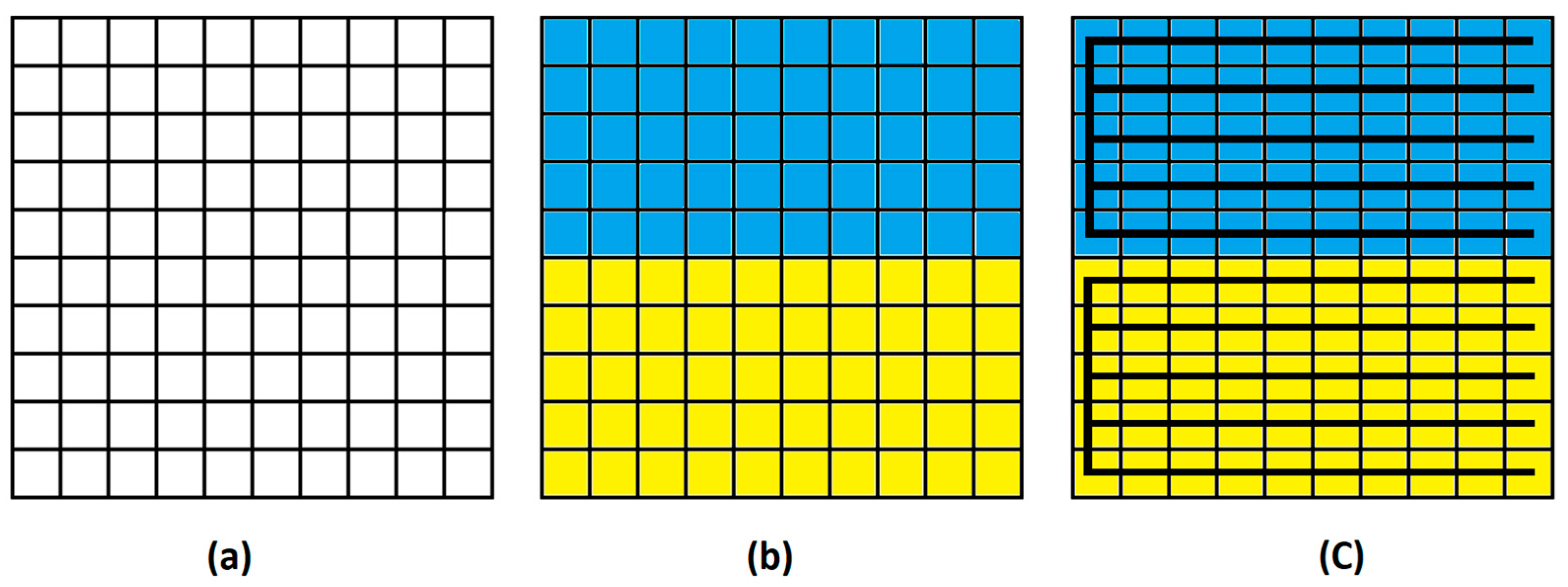
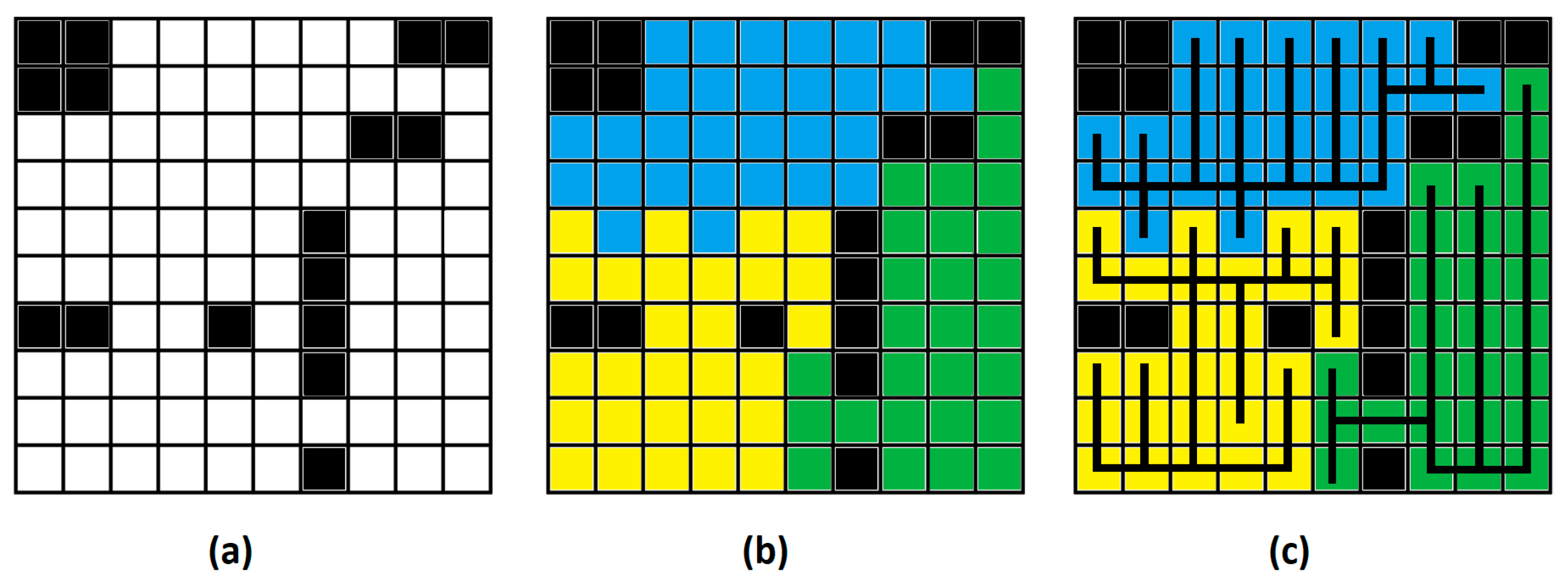
In an optimal situation (Figure 2), the division of the total area would result in perfectly shaped subareas, where each assigned area resembles a rectangle. This form, due to its linearity and simplicity, inherently facilitates the operation of the employed UGVs and leads to optimal navigation paths. An example of an ideal area division with a minimum number of turns is depicted in Figure 3. It is worth noting, however, that in realistic situations where more than two UGVs are employed for a task, and the environment contains irregularly shaped paths and numerous obstacles, regular area division algorithms and ST generators cannot work. A more realistic environment is visualized in Figure 2, where the number of robots is increased to three, and obstacles are introduced to the environment.

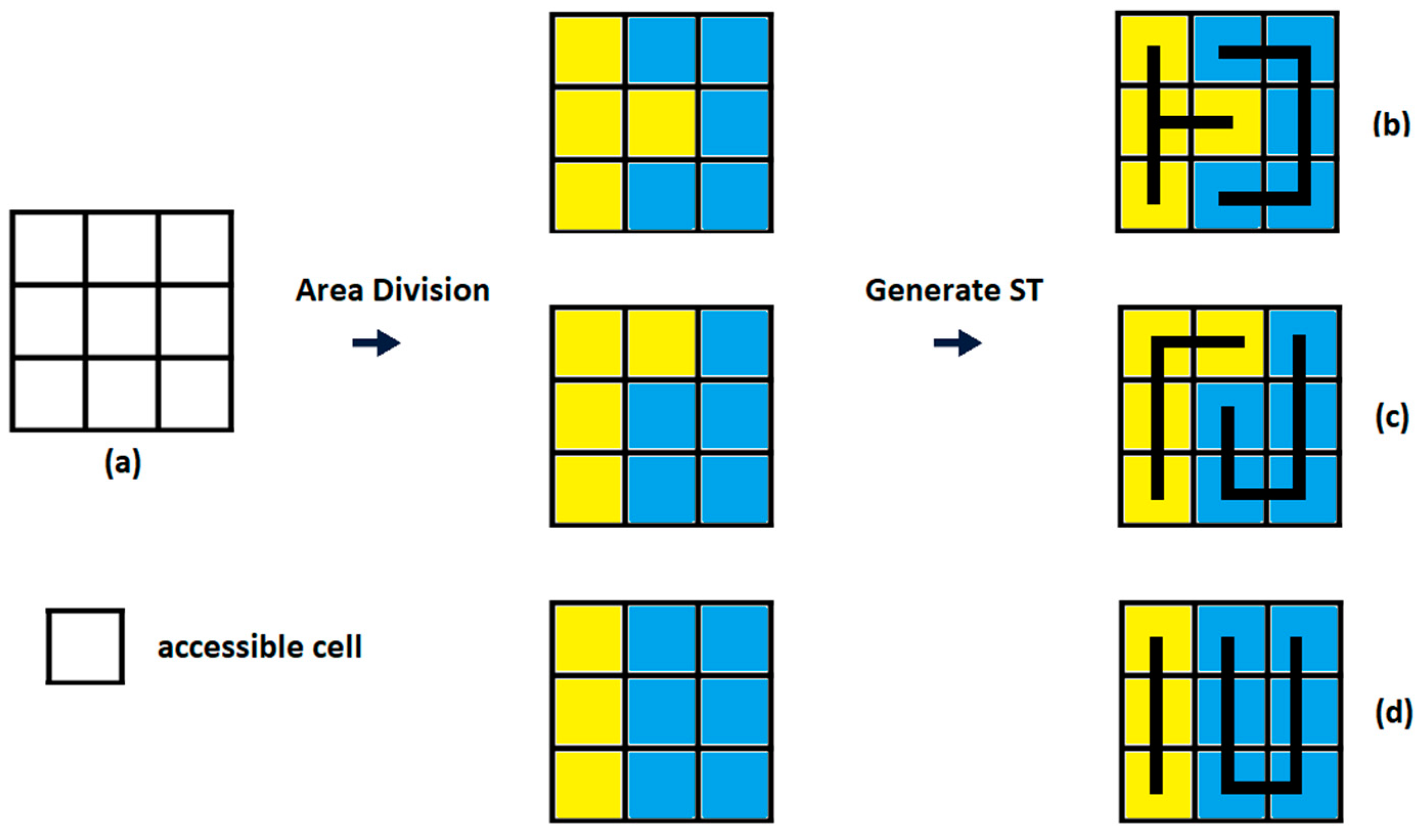
The proposed algorithm is able to reduce the number of turns within each subarea. Such minimization results in an efficient, streamlined coverage path for each UGV, leading to substantial energy savings, enhanced productivity, and an overall optimized performance of the multi-UGV system. It is worth noting that even in equally sized subareas, the generated STs could lead to potentially more or fewer turns for the UGVs (Figure 4).

The main objective of the fine-tuning process is to reduce a phenomenon known as “area blending”. In the context of multi-UGV CPP, and more specifically, area division, area blending refers to the number of cells that belong to a specific cluster, but their neighbors belong to another cluster. This phenomenon usually leads to unfavorable trajectories for UGVs, as they may need to perform more turns during their paths, therefore increasing the energy cost and time for the operation. Figure 5 depicts an example of a 3 × 3 environment with area blending.

To overcome this issue, the optimization scheme uses a redistribution strategy based on the proximity characteristics of each cell. In particular, the cells for which three out of four neighbors belong to another group are redistributed. This criterion ensures that only those cells are redistributed, in order to maintain the overall order of the clusters established by using the initial area division algorithm (Algorithm 2).

Algorithm 2: Reduce blending in the originally divided environment

Input: Environment E, Subareas Z, number of subareas n Output: Environment E’, Subareas Z’ for i from 1 to M do -for j from 1 to N do --cell = E [i, j] --Check only non-boundary cells. --if i > 1 and i < M and j > 1 and j < N then ---cluster_count = empty Dictionary (Find number of neighbors) ---for k from −1 to 1 do ---- for l from −1 to 1 do -----Exclude the cell itself -----if not (k == 0 and l == 0) then ------neighbor_cluster = E [i + k, j + l] ------if neighbor_cluster in cluster_count then -------cluster_count [neighbor_cluster] += 1 ------else -------cluster_count [neighbor_cluster] = 1 ---max_cluster = key of maximum value in cluster_count ---Check if the maximum neighboring cluster has 3 neighbors ---if max_cluster!= cell and cluster_count [max_cluster] >= 3 then ----E [i, j] = max_cluster return E

This fine-tuning process is repeated iteratively until no further beneficial reallocations are identified, resulting in a set of well-defined, contiguous subareas for each UGV. The outcome of this process is a significant reduction in area blending, leading to more efficient coverage paths and reduced energy expenditure.

While this fine-tuning process adds a degree of complexity to the area division stage of the proposed algorithm, it is an essential component of the overall solution. By taking the time to refine the subareas at this stage, the proposed algorithm sets the stage for the subsequent generation of efficient coverage paths, which will be discussed in the following sections.

4.2. Node Exchanging

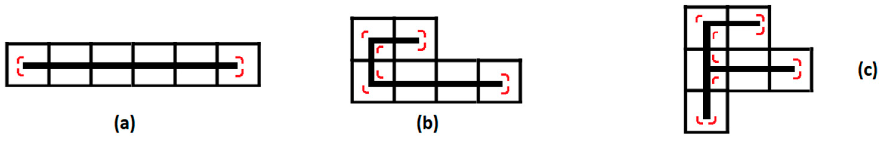
Even though the process mentioned in the previous subsection performs a subarea fine-tuning and reduces area blending within the clusters, the shapes of the new subareas are not further modified. As shown in Figure 4, differently shaped subareas can have a higher or lower number of turns. This section aims to detect problematic shapes within the STs of the subareas and exchange them with the neighboring ST. In each ST, only an ending node (EN) can be exchanged. Depending on the shape of the ST, the ENs can be categorized as follows (Figure 6):

• Linear terminal node (LTN): In this configuration, the node results in a total of two directional alterations. Upon its removal, the path still retains the same number of turns, indicating no change in the overall turning count.
• Angular terminal node (ATN): Initially, this node structure results in a total of four directional shifts. However, when this particular node is eliminated from the path, the total turn count is reduced to two, demonstrating a decrease in the overall number of turns.
• Intersection terminal node (ITN): This node configuration leads to four turns in the initial path structure. Interestingly, the elimination of this node results in the complete eradication of turns, thereby reducing the total turn count to zero.

To minimize the number of turns in the resulting paths, the NE mechanism iterates on the generated STs and performs the following process:

• Each NE indicates that one subarea relinquishes an end node, which is subsequently adopted by a different (neighboring) subarea.
• Prioritization is accorded during the node-discarding process, where ITNs are discarded first, followed by ATNs. The discarded node, now assimilated by an adjacent subarea, integrates into a new ST, forming a modified shape at the end node. Ideally, LTNs are preferred, ATNs are the next best option, and ITNs are considered the least desirable to minimize the turn count. Following this, the said adjacent subarea discards an end node to a different subarea, and this process continues in a cyclic manner. After the completion of a cycle, the count of nodes associated with the related subarea approximates (n/nr). If the number of turns fails to satisfy Equation (16), the current exchange cycle is discarded, and a new one is initiated.
• Every node eligible for exchange in a subarea undergoes an exchange before moving on to the subsequent subarea.
• The NE process is terminated when further exchanges cease to reduce the total number of turns within the specified area of interest, or when the maximum iteration count is reached.

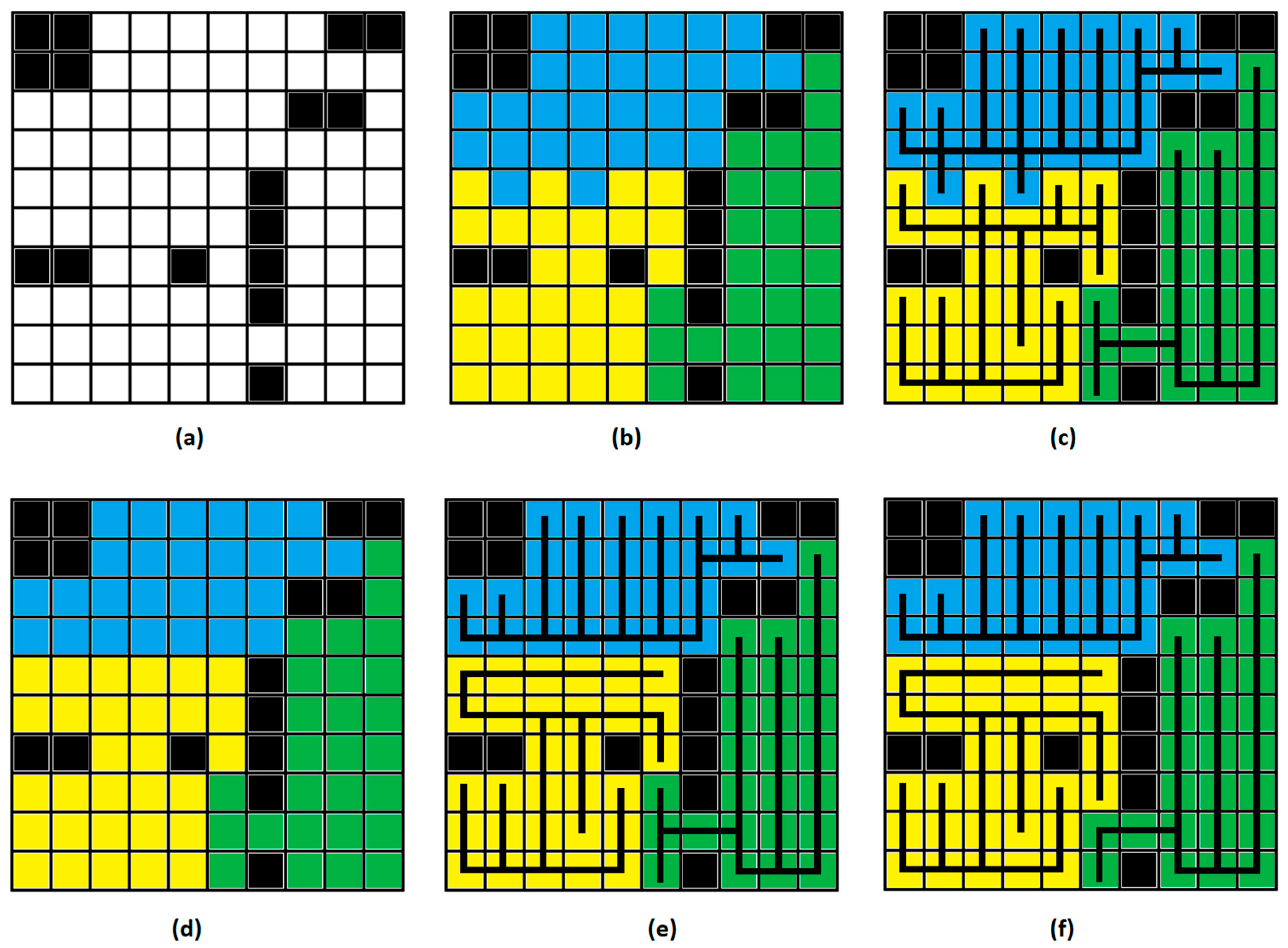
A visual representation of the NE process is depicted in Figure 7 (along with the previous steps).

5. Experimental Results

In this section, we present the empirical outcomes of the extensive testing and validation of the proposed methodology, conducted using a robust computational framework implemented in C# (version 11) and Java (version 19). These programming languages were chosen due to their capacity to handle the intricate operations, data structures, and interactions inherent in our multi-UGV CPP solution. The computational experiments were carried out on an Intel Core i7 8700K processor with 16 gigabytes of random-access memory (RAM), providing the necessary computational power to run our resource-intensive simulations.

The proposed methodology proved to be proficient in reallocating UGV subareas and fine-tuning the generated STs to minimize the number of turns within a trajectory. This was compared with A*-DARP+STC [25] and [17]. The simulation environment adopted was similar to [20] and consisted of three similar-sized (64 × 64) environments each showcasing unique features. The obstacle ratios of environments (a), (b), and (c) were 10.1%, 29.6%, and 43.5%, respectively. These environments were generated employing a pseudo-random process, resulting in a distinct mix of accessible regions and obstacles.

Table 1. Experimental results for environments (a), (b), and (c).

		A*-DARP + STC [25]	[17]	AP + Kruskal + Optimization
Env.	UGVs	Total Turns	Total Turns	Total Turns	Reallocated Cells + NE
a	3	522	545	485	12
	4	510	532	476	8
	5	469	459	430	7
b	3	564	543	492	13
	4	530	489	470	14
	5	523	435	493	8
c	3	456	498	401	7
	4	440	464	405	8
	5	442	540	424	5

presents the findings of the simulations.

As shown in Table 1, the experimental results confirm that our proposed methodology consistently surpasses the performance of the comparison methods in terms of reducing the total number of turns. For instance, in environment “a” with three UGVs, which had an obstacle ratio of 10.1%, our methodology achieved a total of 485 turns, outperforming A*-DARP + STC and methods developed in [25], which resulted in 522 and 545 turns, respectively. Furthermore, it is noteworthy that these improvements in turn reduction were accomplished with only a modest number of cell reallocations, underscoring the efficiency of our fine-tuning process. Similar patterns of superior performance of our algorithm were observed across the different environments.

The spatial distribution of obstacles and the initial placement of UGVs, particularly in algorithms that support initial positioning, can considerably influence the effectiveness of the area division and ST generation. These variables hold significant sway over the current algorithms’ capacity to reduce the number of turns of trajectories. There are instances in which, due to the intricate interplay between the layout of obstacles and the initial positioning of UGVs, no further reduction in turns is achievable. Even though this is difficult to prove, an example of such a case can be visualized (Figure 1). This realization underscores the crucial role these factors play in the planning process and the need for algorithms to be adept at handling a wide variety of terrain configurations and initial conditions. Such intricacies in the optimization landscape only add to the richness of the problem at hand and reinforce the need for robust, adaptive, and intelligent multi-UGV CPP methodologies, such as the one proposed in this study.

6. Discussion on Energy Efficiency

In the context of UGV CPP, energy efficiency stands as a complex and multifaceted challenge. Unlike traditional modes of vehicular motion where energy expenditure predominantly depends on distance or speed, UGVs, particularly in CPP applications, present a unique energy consumption profile. The overall energy consumption is influenced by various intricate factors, such as the nature of the movement (straight or turning), terrain characteristics, and sudden changes in the operational landscape, among others.

Optimizing energy utilization in this context requires an understanding of the interplay of these factors and designing a solution that effectively accounts for them. In our proposed approach, we sought to tackle this complexity by aiming to reduce the number of turns in the final coverage paths of the UGVs. This strategy is based on a key insight: most UGVs, in general, consume more energy when performing a turn than when moving in a straight line. The increased energy consumption during turns is primarily because these maneuvers typically require the UGVs to decelerate, stop, and then accelerate again.

To illustrate, let us consider two coverage paths of equal distance D. One path contains X turns, and the other contains $Y$ turns, where $X\times Y$. Often, the energy consumption of the path with $X$ turns would be higher due to the additional energy expenditure during turning. The exact amount of energy saved by reducing the number of turns can vary widely depending on specific UGV specifications. UGVs with larger turning-to-straight movement energy ratios will typically benefit more from the minimization of turns, while other UGVs with smaller ratios will benefit less. One example of UGVs with larger benefits is the UGVs that are commonly used in agricultural applications. Due to the nature of the terrain, these UGVs have higher energy requirements when turning than when moving in straight lines.

A potential formula that can be used to quantify the total energy consumption per UGV path is as follows:

$$E=E_{cs}\times D_{cs}+E_T\times D_T$$

(17)

where $E_{cs}$ is the energy consumption of the UGV during cruising speed, $D_{cs}$ is the distance (cells) traversed using cruising speed, $E_T$ is the energy consumption of the UGV when turning, and $D_T$ is the number of turns of the UGV.

A more sophisticated formula that would yield more precise energy calculations would consider the acceleration and deceleration of the UGV and its energy consumption in the following states:

$$E=E_{cs}\times D_{cs}+E_{DS}\times D_{DS}+E_{AS}\times D_{AS}+E_T\times D_T$$

(18)

where $E_{DS}$ is the energy consumption of the UGV during deceleration (when preparing to take a turn), $D_{DS}$ is the distance (cells) traversed during deceleration, $E_{AS}$ is the energy consumption of the UGV when accelerating (after a turn), and $D_{AS}$ is the distance covered (cells) while accelerating.

The distinctiveness of our methodology resides in the integration of a terrain-aware cost function coupled with an adaptive path replanning module. These components cohesively assimilate the energy-influencing parameters to engineer paths that potentially consume less energy. It is important to note that the proposed paradigm predominantly diminishes the energy expenditure of a UGV path, contingent upon the assumption that the UGV incurs significant energy costs during turning maneuvers. Although the current study does not offer explicit quantitative measures of energy efficiency, it delineates a fundamental foundation for future empirical investigations. Thus, our research marks a critical milestone toward the conceptualization and execution of energy-centric CPP strategies in multi-UGV contexts.

7. Conclusions

In this study, we presented an innovative approach to address the challenge of the multi-UGV CPP problem with a particular emphasis on optimizing UGV energy utilization through effective area fine-tuning. Our methodology, which hinges upon the optimization of assigned areas and the generated STs, revealed its potential to significantly enhance the energy efficiency of CPP for multi-UGV scenarios.

The resultant algorithm outperformed the existing methodologies in terms of area division optimization and turn reduction, demonstrating its robustness through a series of comprehensive simulations. Notably, our adaptive path replanning module ensured a higher degree of flexibility and effectiveness, particularly in challenging terrain conditions. The work delineated here presents substantial contributions to the field of CPP and provides a promising foundation for future research efforts aimed at further augmenting the efficiency and endurance of multi-UGV operations.

As we contemplate future enhancements to our methodology, one aspect of paramount interest is the extension of the algorithm to accommodate environments with predictable moving obstacles. Such a modification would necessitate the introduction of the time variable into the planning algorithm. By assessing the capabilities of UGVs, particularly their moving and turning speeds, the algorithm could be designed to anticipate the location of a given obstacle at a particular time, thus ensuring that the generated path is consistently clear of obstacles. This adaptation would likely entail substantial modifications to our current approach, especially concerning the spanning tree generation algorithm and the node exchange procedure. By incorporating the time dimension into our planning algorithm, we can unlock new realms of versatility for multi-UGV CPP, opening doors for even greater efficiency and adaptability in complex and dynamic operational scenarios.