Author Contributions
Conceptualization, T.R., K.T., P.K., B.K. and Y.I.; methodology, T.R., K.T. and P.K.; software, T.R. and K.T.; validation, T.R., K.T., P.K. and B.K.; formal analysis, T.R., K.T. and P.K; investigation, T.R., K.T., P.K., B.K., Y.I. and S.F.; resources, Y.I., S.F. and K.N..; data curation, Y.I., S.F. and K.N.; writing—original draft preparation, T.R.; writing—review and editing, T.R., P.K. and B.K.; visualization, T.R.; supervision, P.K., B.K., Y.I. and S.F.; project administration, T.R., K.T., P.K. and Y.H.; funding acquisition, Y.I. and Y.H. All authors have read and agreed to the published version of the manuscript.
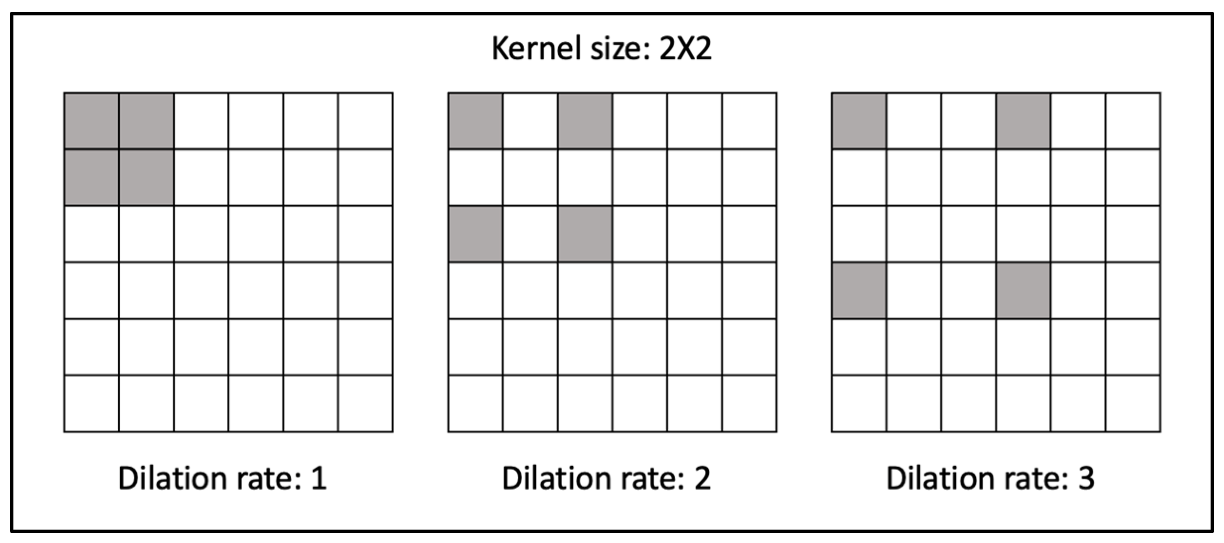
Figure 1.
Example of dilated convolution kernel with rates 1, 2, and 3.
Figure 1.
Example of dilated convolution kernel with rates 1, 2, and 3.
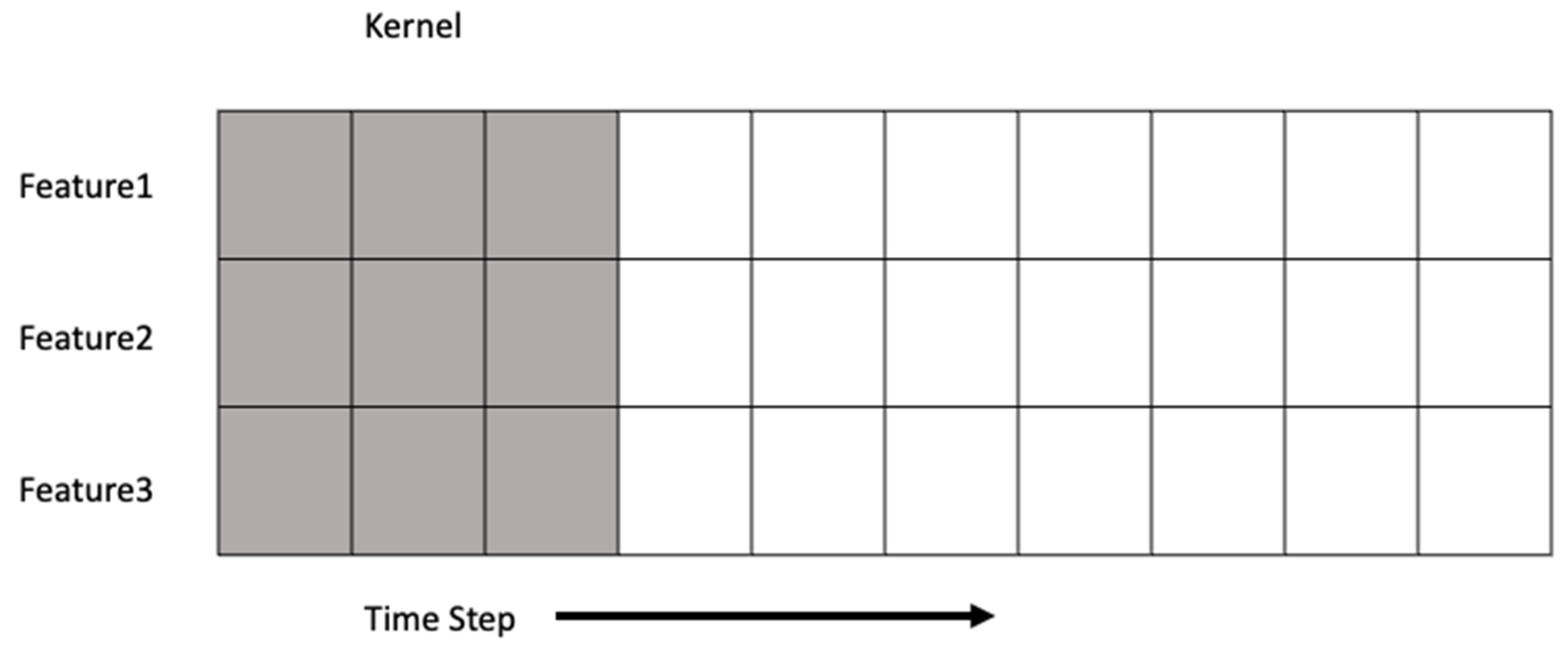
Figure 2.
The characteristics of CONV1D neural network.
Figure 2.
The characteristics of CONV1D neural network.
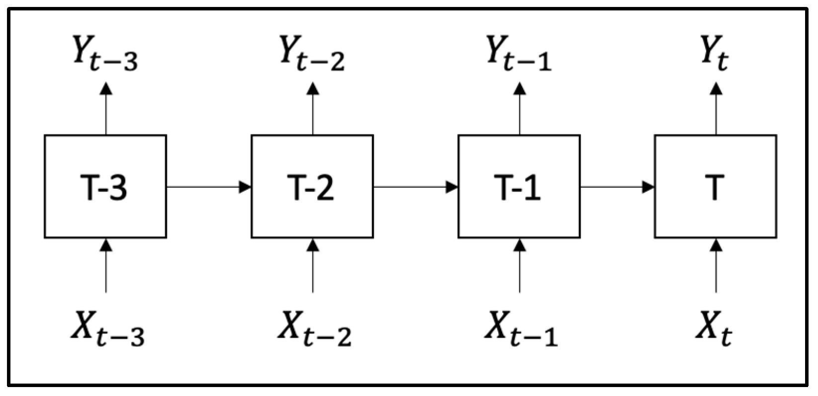
Figure 3.
Recurrent Neural Network.
Figure 3.
Recurrent Neural Network.
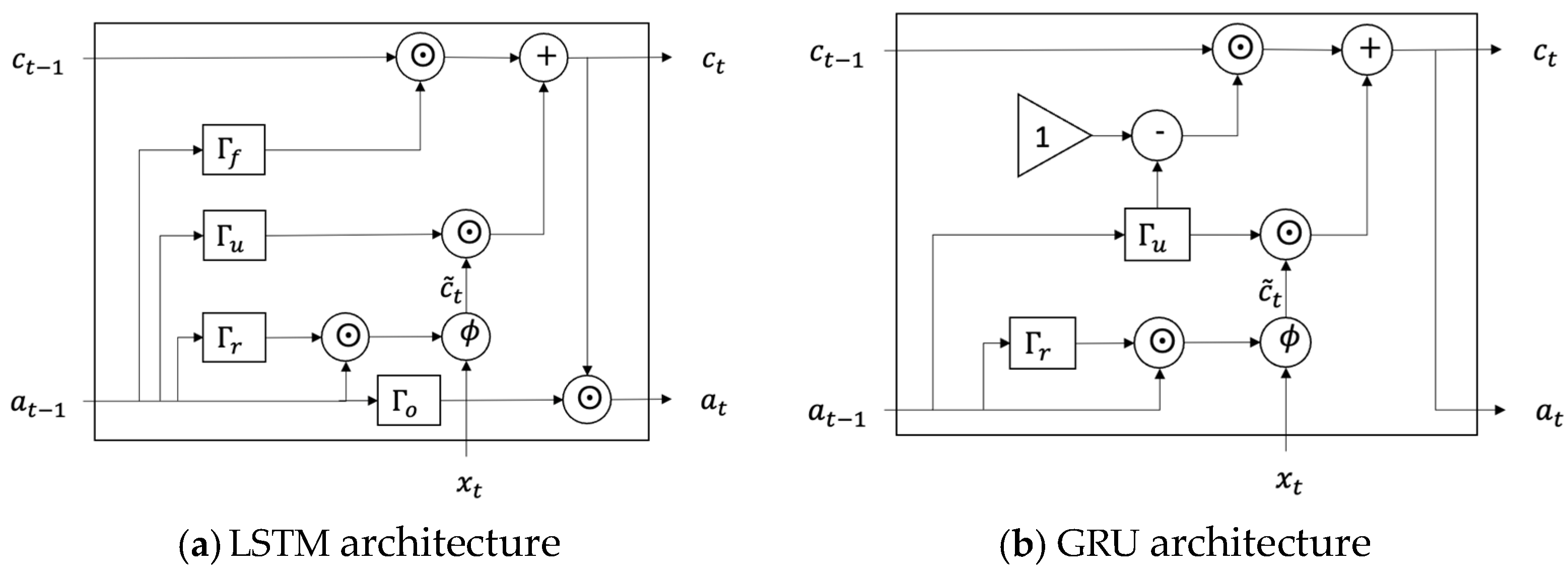
Figure 4.
LSTM architecture (
a) and GRU architecture (
b) [
27].
Figure 4.
LSTM architecture (
a) and GRU architecture (
b) [
27].
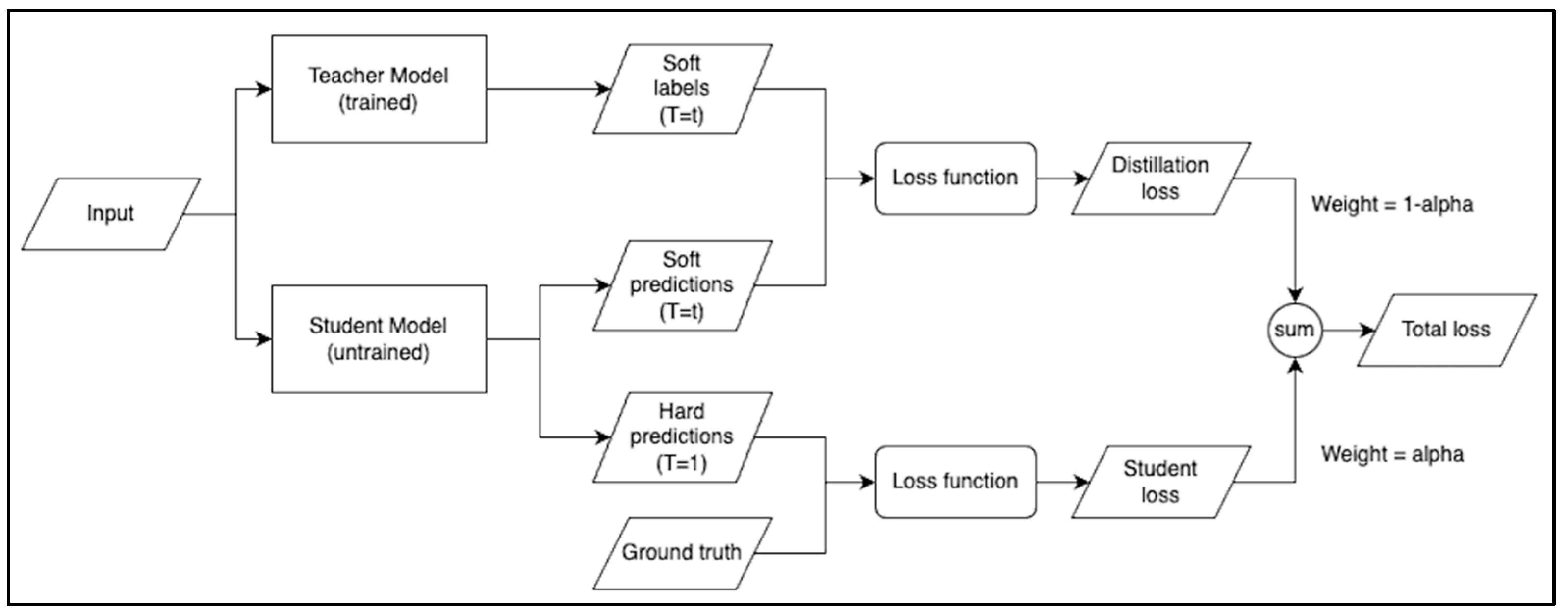
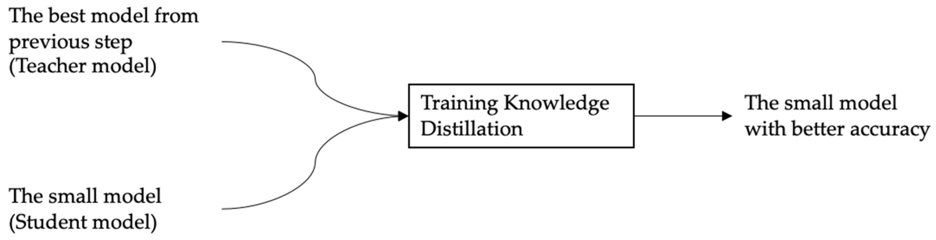
Figure 5.
An overview of knowledge distillation.
Figure 5.
An overview of knowledge distillation.
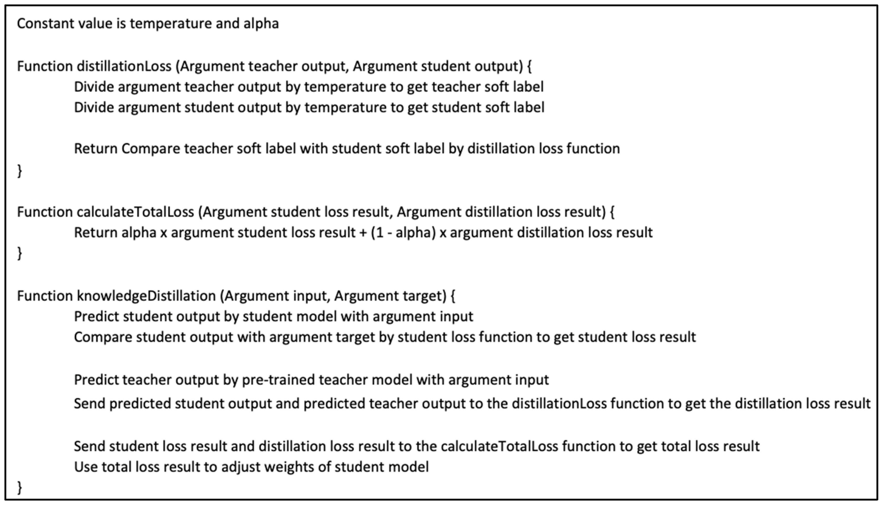
Figure 6.
A pseudo code of knowledge distillation.
Figure 6.
A pseudo code of knowledge distillation.
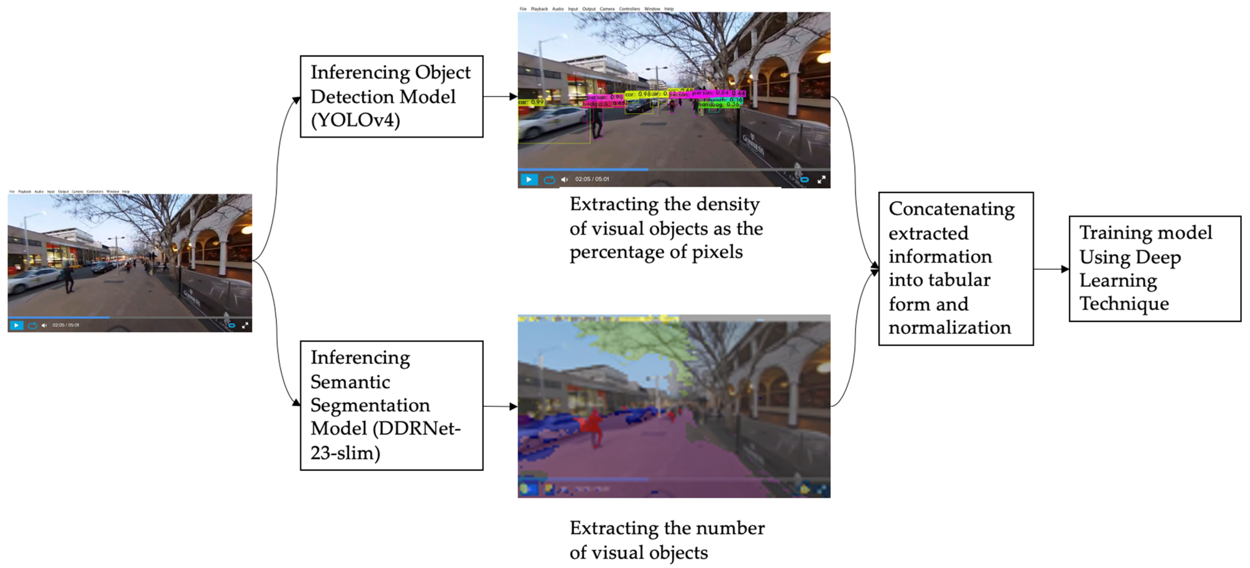
Figure 7.
The overview of “the” QoL inference step.
Figure 7.
The overview of “the” QoL inference step.
Figure 8.
The overview of “the” knowledge distillation step.
Figure 8.
The overview of “the” knowledge distillation step.
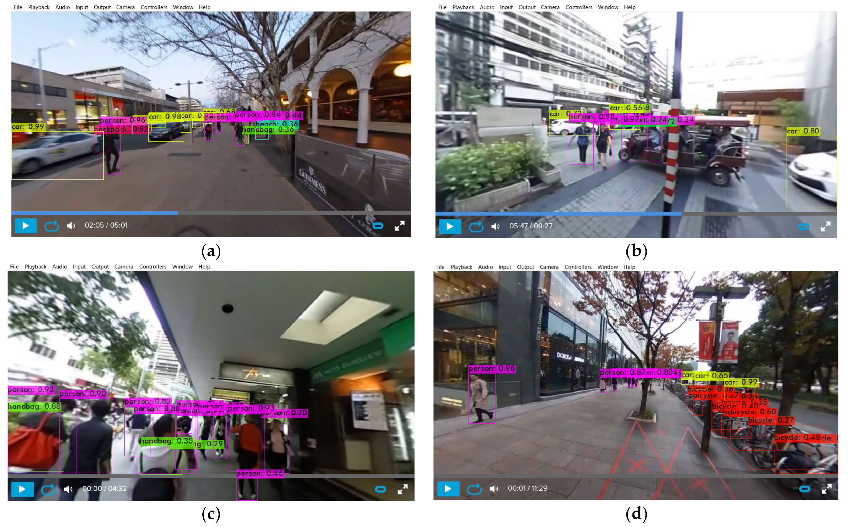
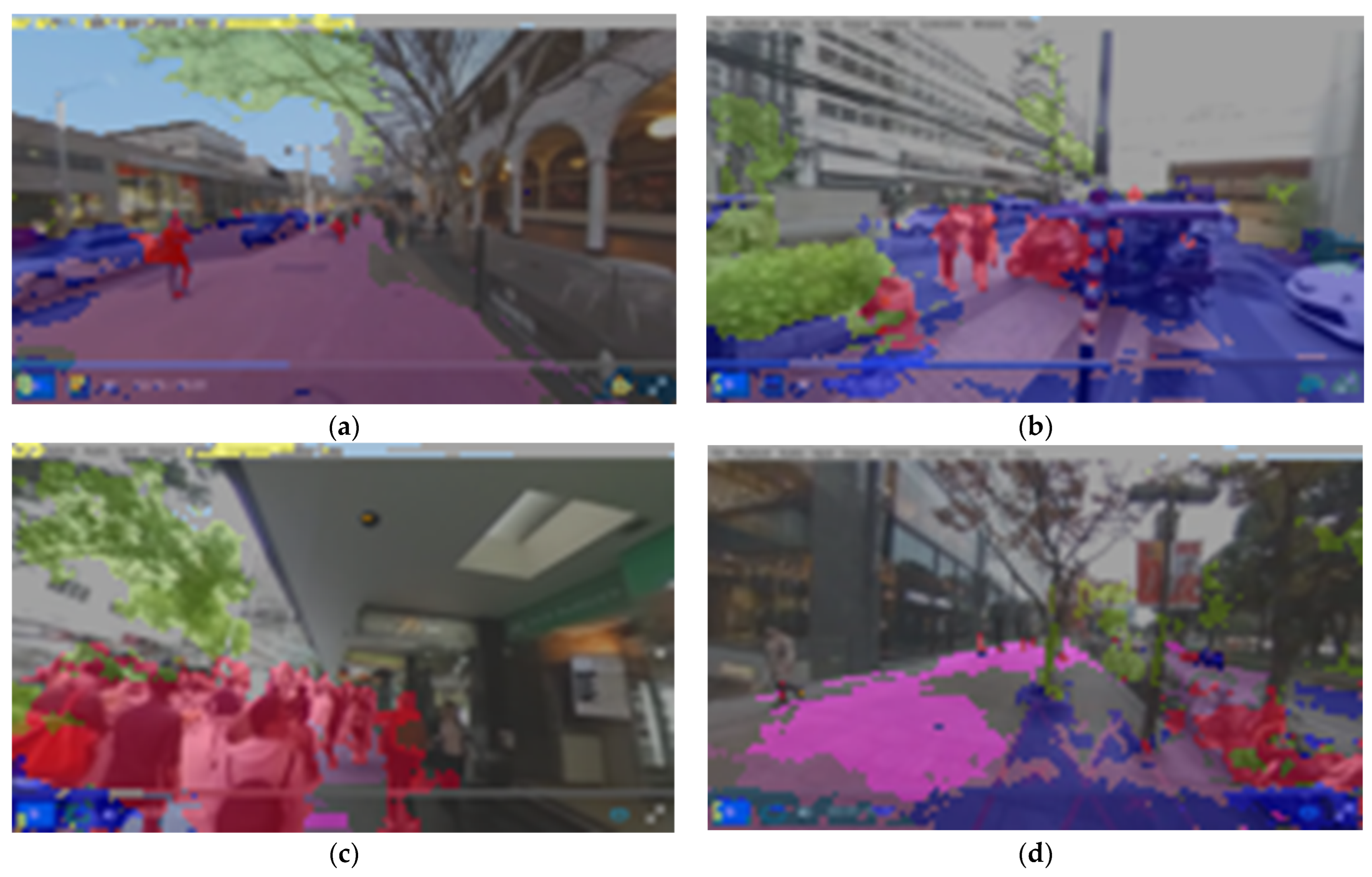
Figure 9.
Example of the results from YOLOv4. (a) Canberra; (b) Bangkok; (c) Brisbane; (d) Sakae.
Figure 9.
Example of the results from YOLOv4. (a) Canberra; (b) Bangkok; (c) Brisbane; (d) Sakae.
Figure 10.
Example of the results from DDRNet-23-Slim. (a) Canberra; (b) Bangkok; (c) Brisbane; (d) Sakae.
Figure 10.
Example of the results from DDRNet-23-Slim. (a) Canberra; (b) Bangkok; (c) Brisbane; (d) Sakae.
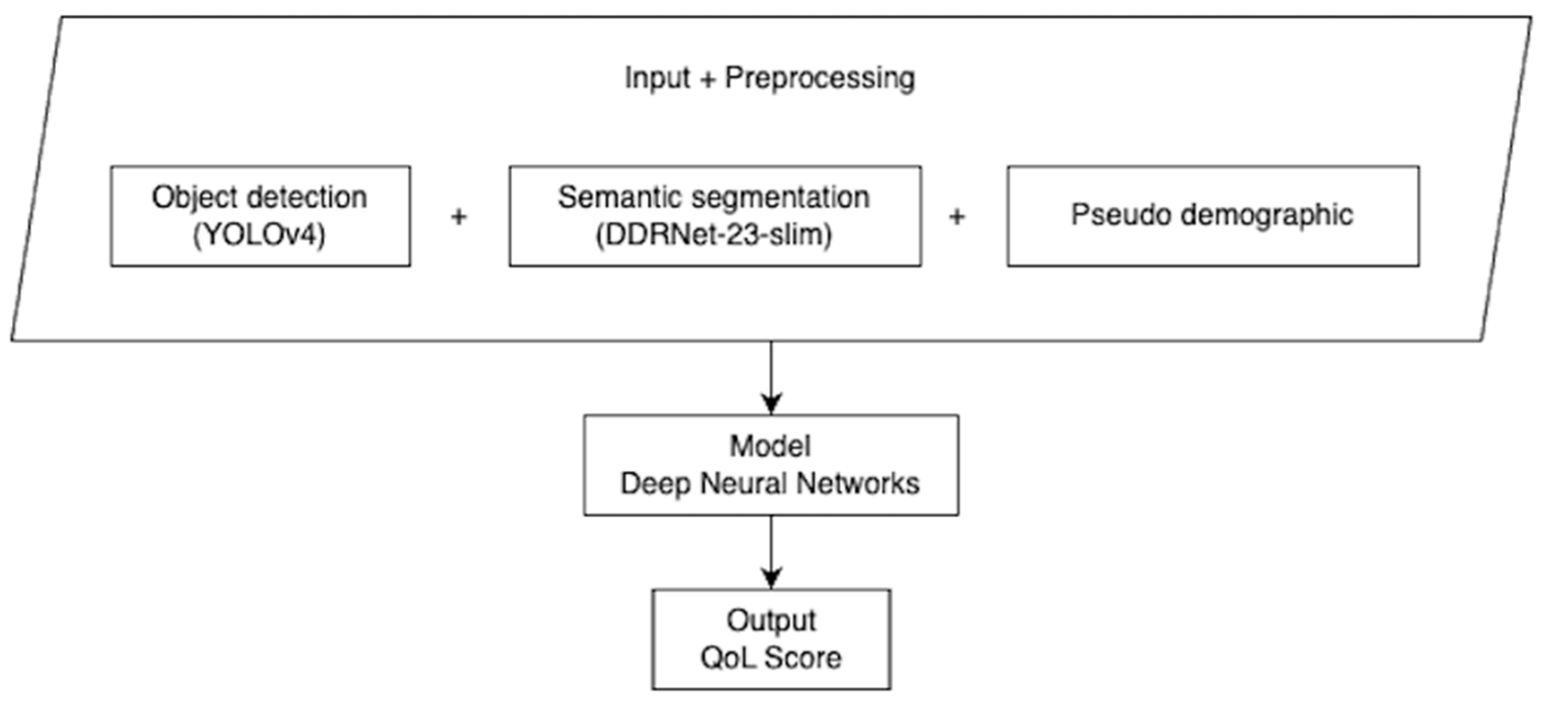
Figure 11.
Overview of QoL prediction model architecture.
Figure 11.
Overview of QoL prediction model architecture.
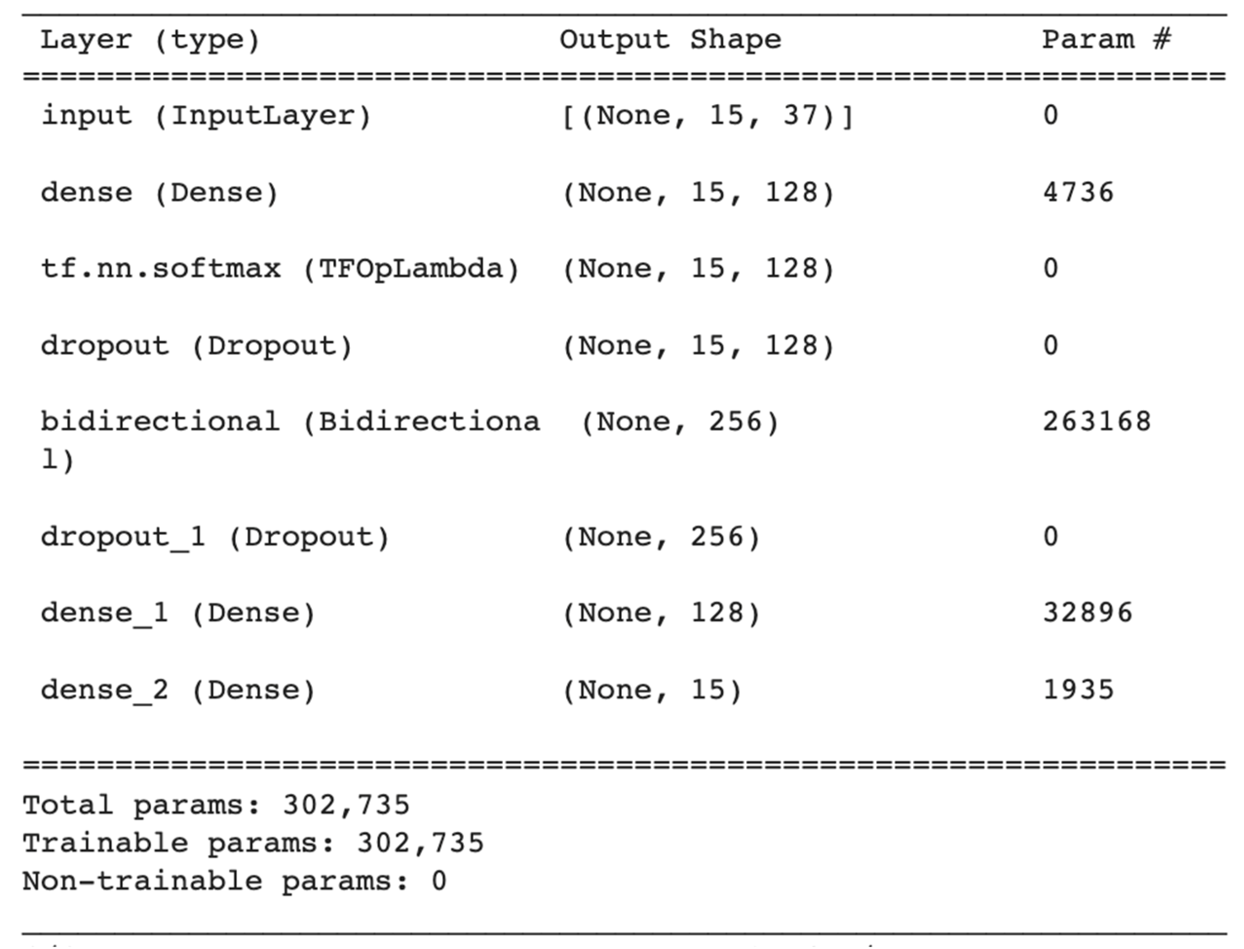
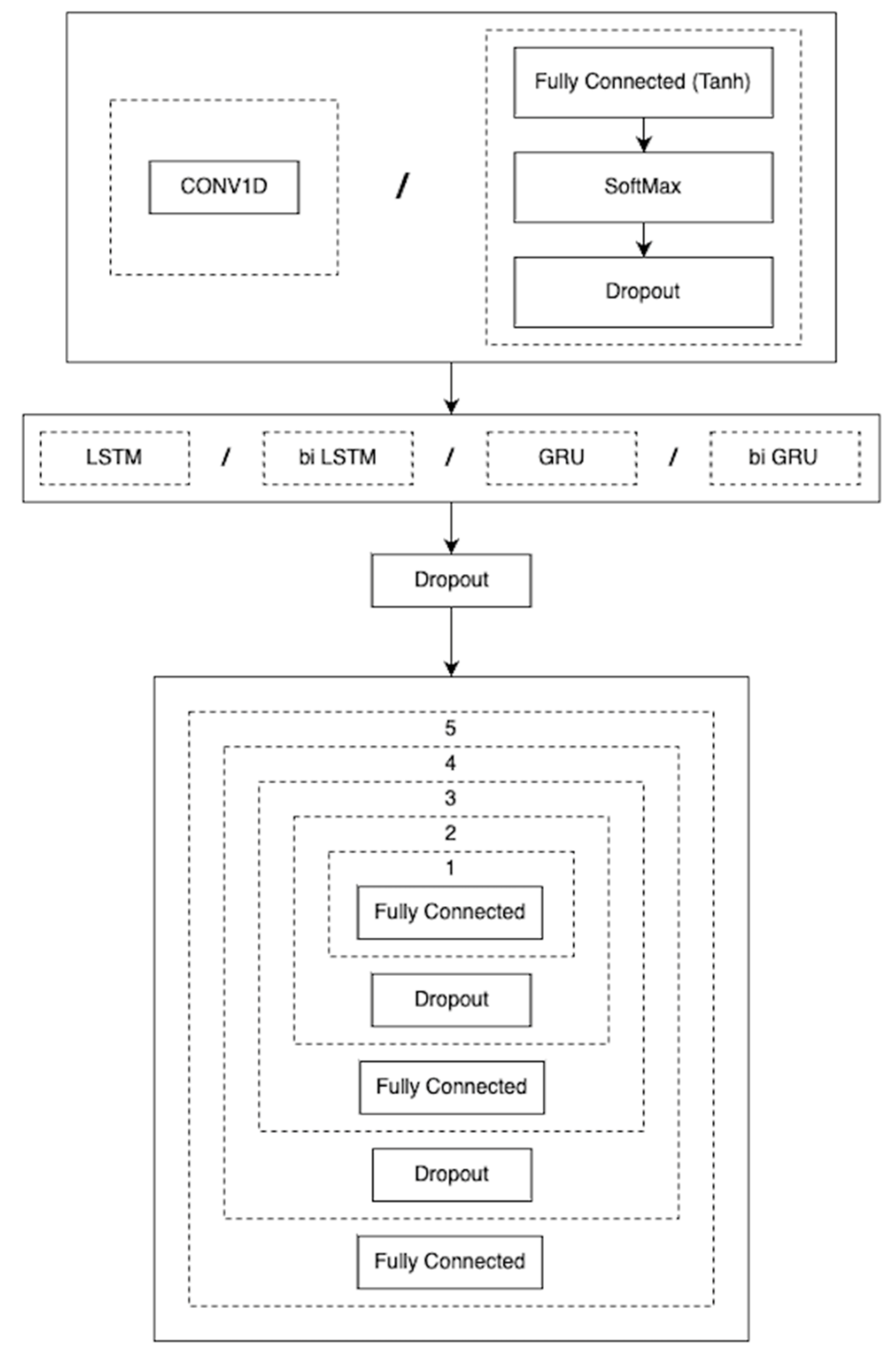
Figure 12.
The architecture of the QoL prediction model selecting the options of CONV1D for the first box and LSTM for the second box.
Figure 12.
The architecture of the QoL prediction model selecting the options of CONV1D for the first box and LSTM for the second box.
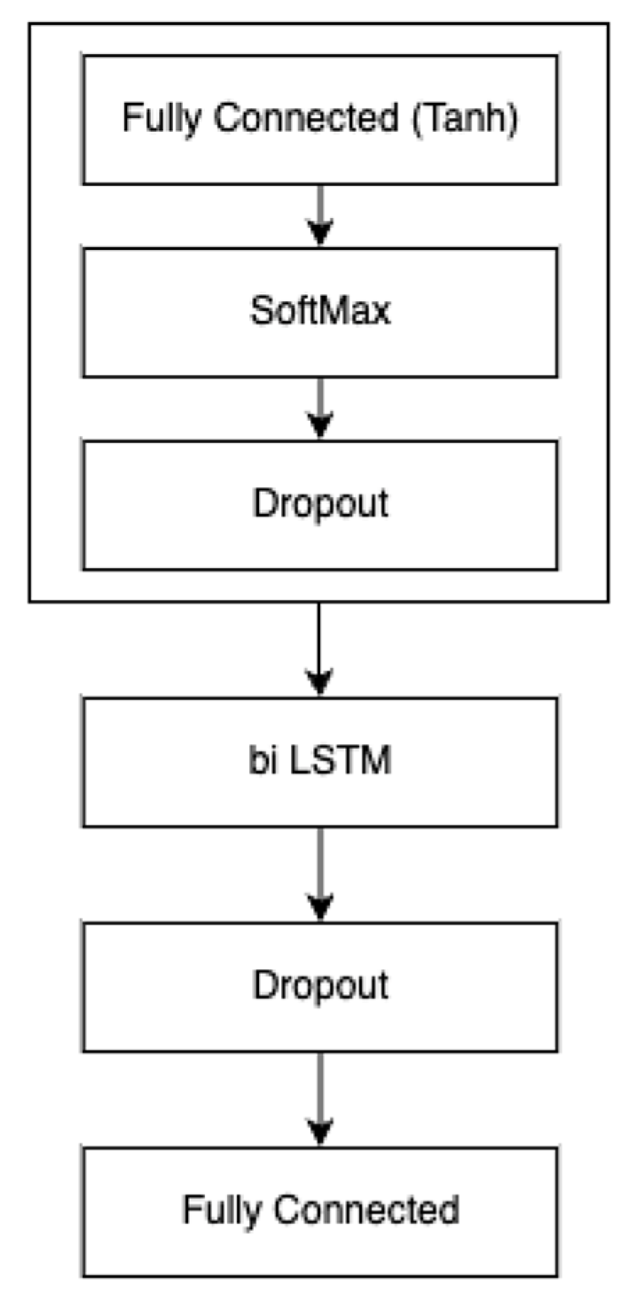
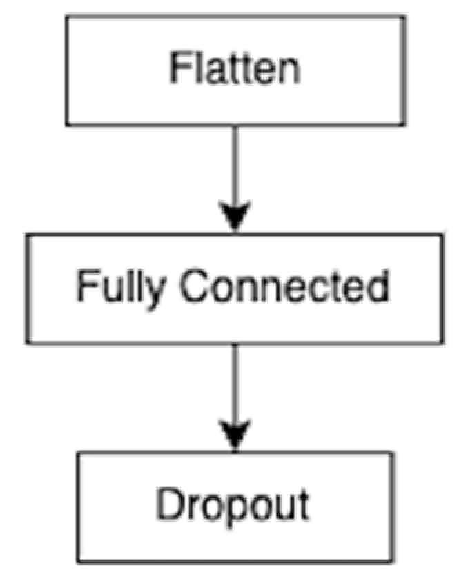
Figure 13.
The QoL prediction model architecture selecting the options of fully connected with the tanh activation function and SoftMax for the first box and LSTM for the second box.
Figure 13.
The QoL prediction model architecture selecting the options of fully connected with the tanh activation function and SoftMax for the first box and LSTM for the second box.
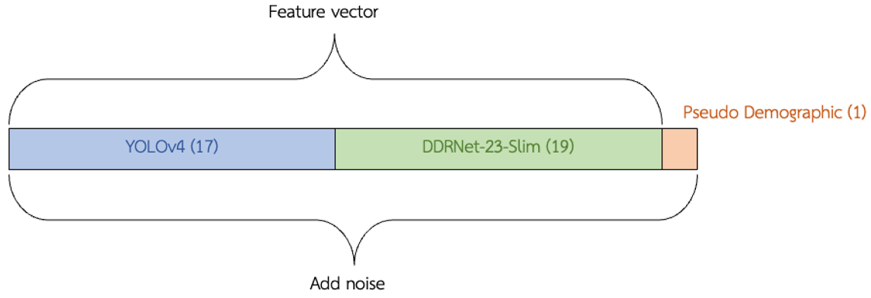
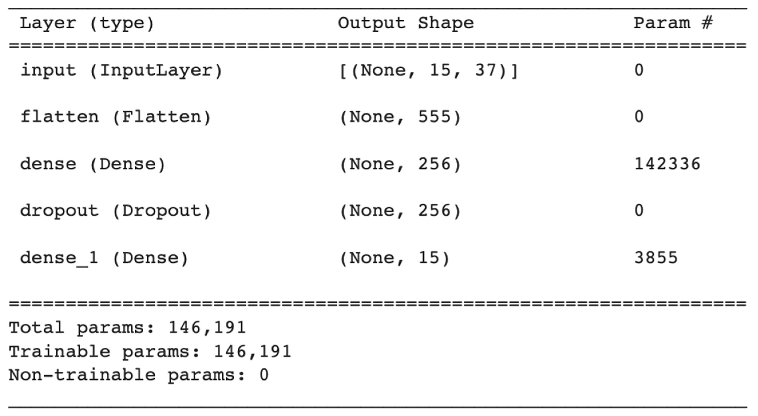
Figure 14.
The input features for the QoL prediction model.
Figure 14.
The input features for the QoL prediction model.
Figure 15.
Input features and output labels in the training process of the QoL prediction model.
Figure 15.
Input features and output labels in the training process of the QoL prediction model.
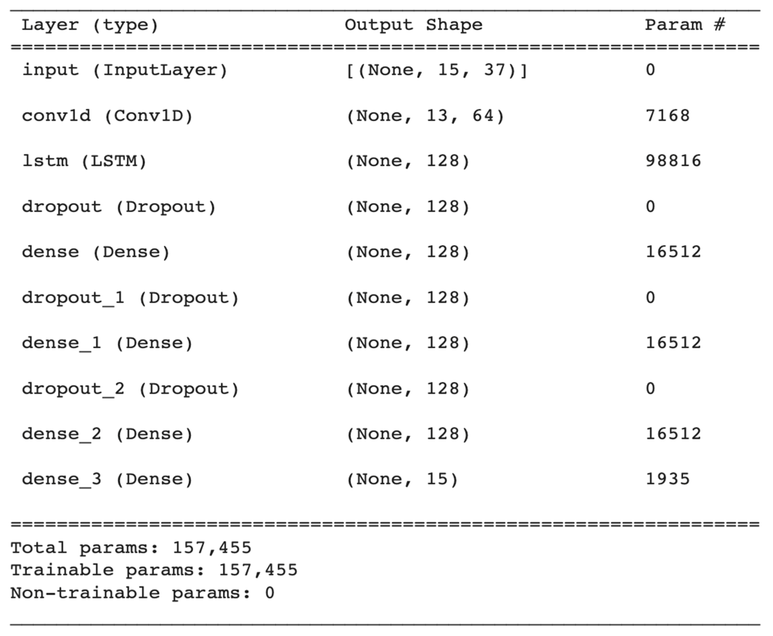
Figure 16.
An architecture of the teacher model training in the knowledge distillation process.
Figure 16.
An architecture of the teacher model training in the knowledge distillation process.
Figure 17.
A configuration of the teacher model training in the knowledge distillation process.
Figure 17.
A configuration of the teacher model training in the knowledge distillation process.
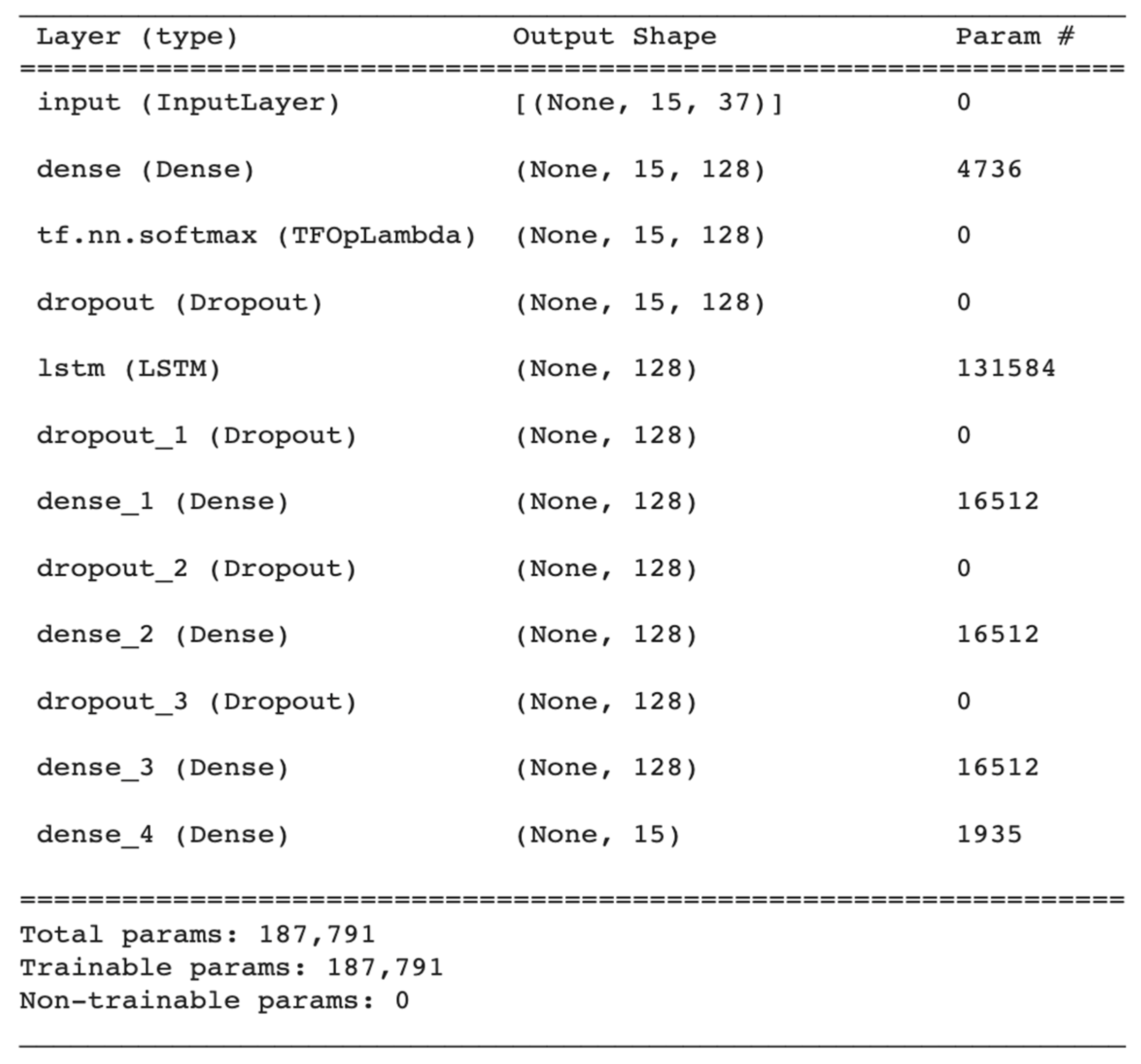
Figure 18.
An architecture of the student model training in the knowledge distillation process.
Figure 18.
An architecture of the student model training in the knowledge distillation process.
Figure 19.
A configuration of the student model training in the knowledge distillation process.
Figure 19.
A configuration of the student model training in the knowledge distillation process.
Figure 20.
An example of loss graphs showing changes in each epoch of model training for the within-the-city experiment group.
Figure 20.
An example of loss graphs showing changes in each epoch of model training for the within-the-city experiment group.
Figure 21.
An example of loss graphs showing changes in each epoch of model training for the across-the-cities experiment group.
Figure 21.
An example of loss graphs showing changes in each epoch of model training for the across-the-cities experiment group.
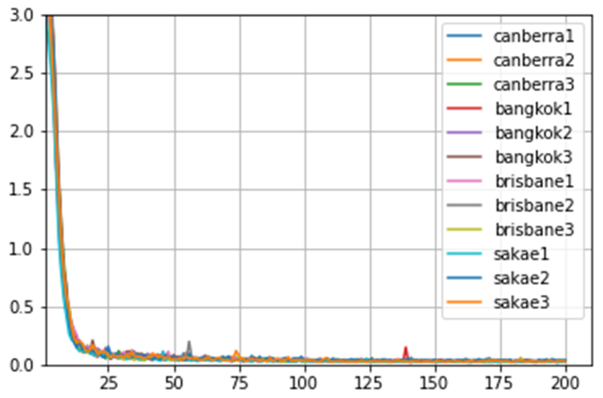
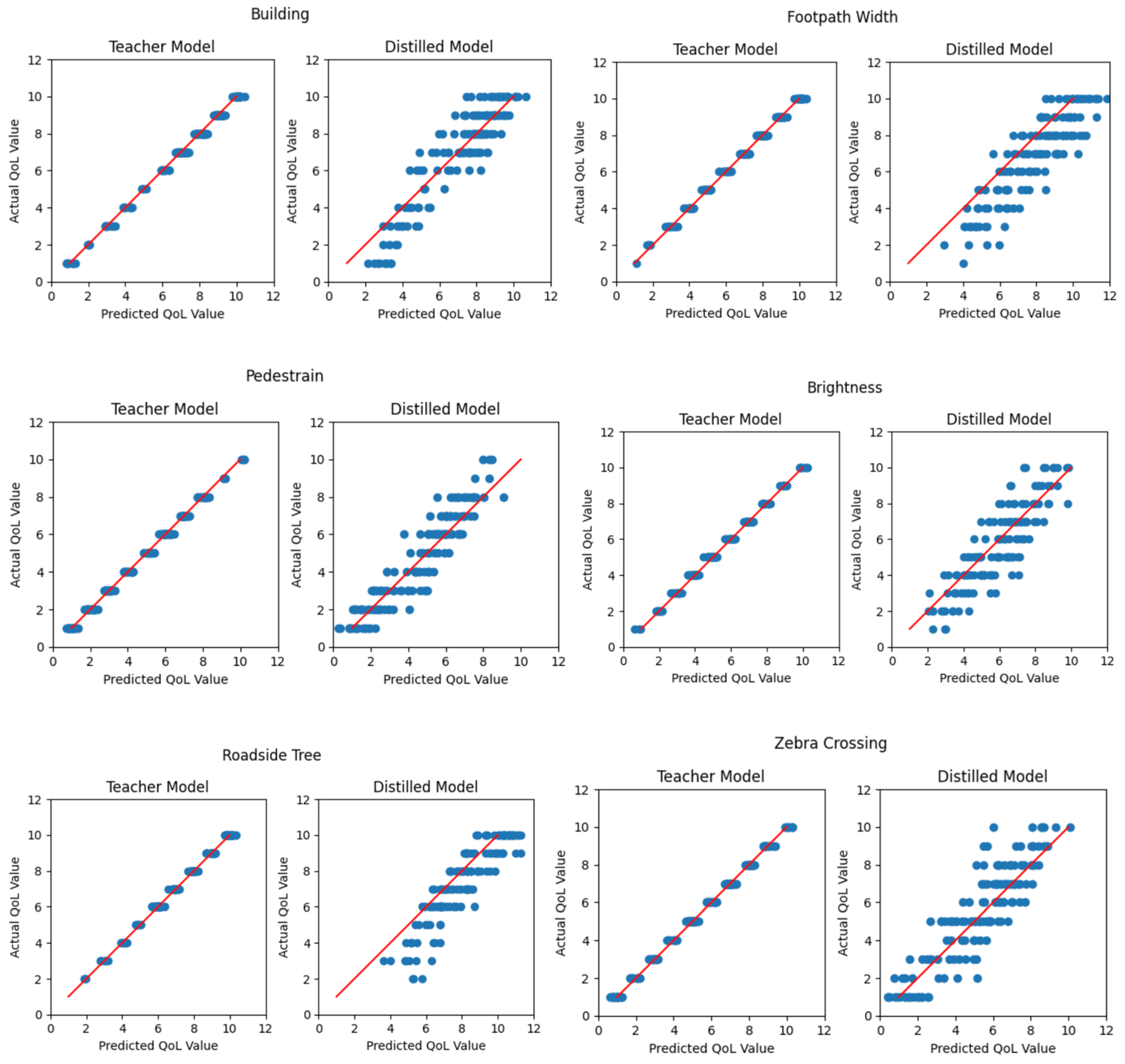
Figure 22.
The comparison graph plots between the teacher and distilled models’ actual results (Y-axis) and predicted results (X-axis) selected from a testing set of Canberra Scene3, within-the-city experiment groups.
Figure 22.
The comparison graph plots between the teacher and distilled models’ actual results (Y-axis) and predicted results (X-axis) selected from a testing set of Canberra Scene3, within-the-city experiment groups.
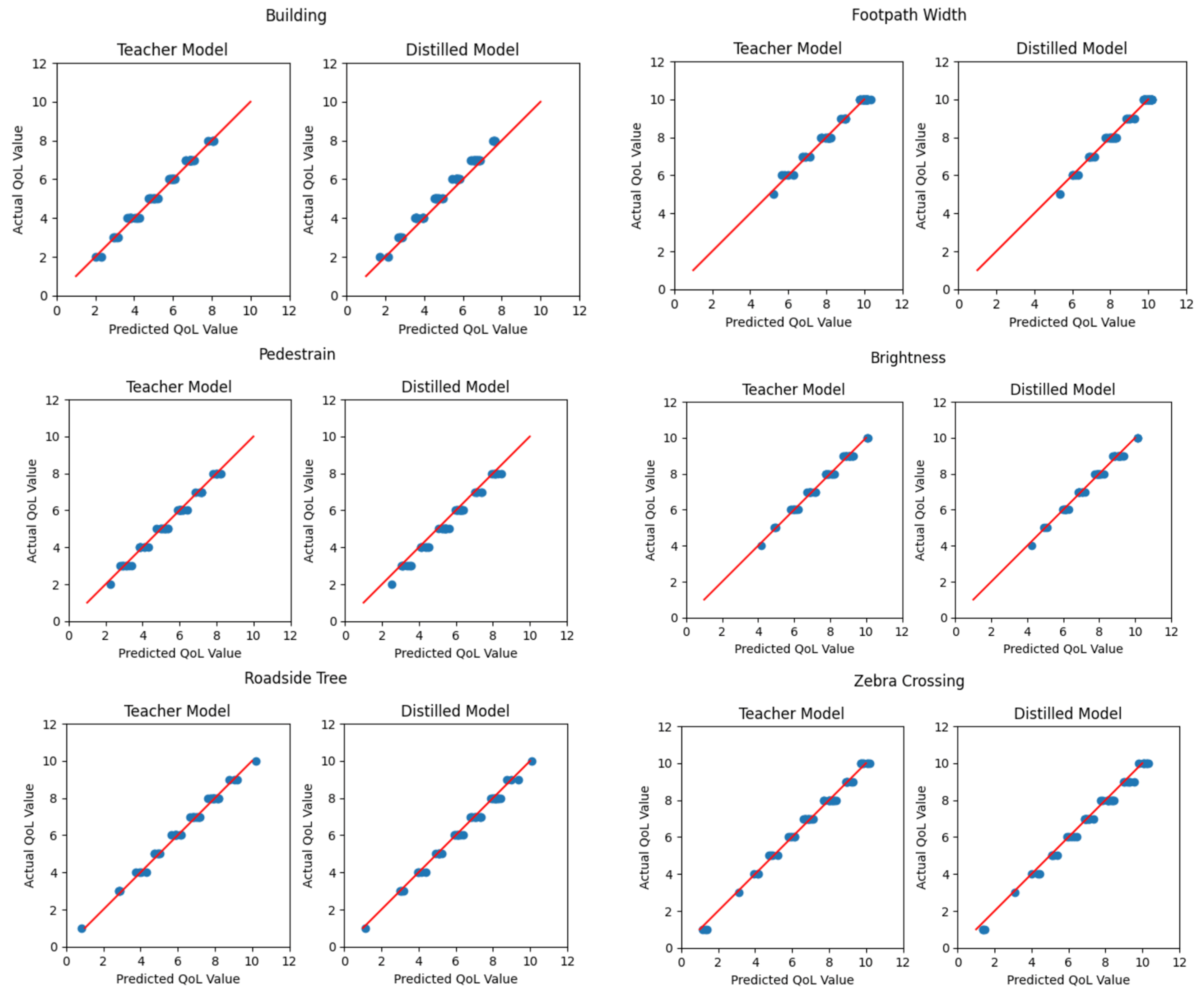
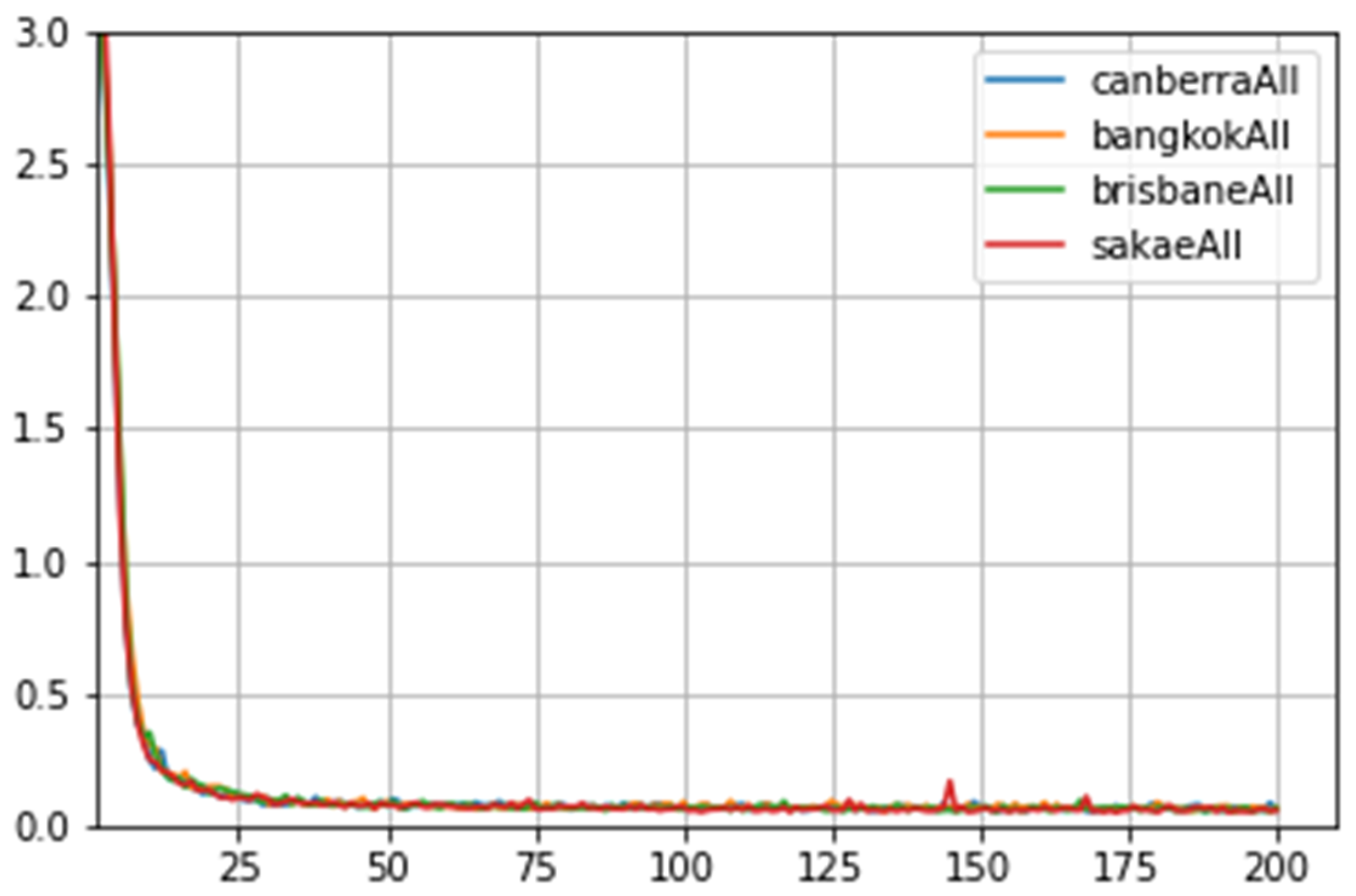
Figure 23.
The comparison graph plots between the teacher and distilled models’ actual results (Y-axis) and predicted results (X-axis) selected from a testing set of Canberra Scene all, across-the-cities experiment groups.
Figure 23.
The comparison graph plots between the teacher and distilled models’ actual results (Y-axis) and predicted results (X-axis) selected from a testing set of Canberra Scene all, across-the-cities experiment groups.
Table 1.
The 15 factors of evaluated score for each respondent in the questionnaire.
Table 1.
The 15 factors of evaluated score for each respondent in the questionnaire.
| Building | Building |
| Facility |
| Roof |
| Activity | Bench |
| Stall |
| Walking or Sitting People |
| Footpath | Footpath Width |
| Pedestrian |
| Brightness |
| Installation | Bicycle Parking |
| Roadside Tree |
| Electric Pole |
| Roadway | Parking |
| Zebra Crossing |
| Traffic Volume |
Table 2.
The result classes from YOLOv4 model.
Table 2.
The result classes from YOLOv4 model.
| 1. Person | 10. Traffic light |
| 2. Bicycle | 11. Fire hydrant |
| 3. Car | 12. Stop sign |
| 4. Motorbike | 13. Parking meter |
| 5. Aeroplane | 14. Bench |
| 6. Bus | 15. Backpack |
| 7. Train | 16. Umbrella |
| 8. Truck | 17. Handbag |
| 9. Boat | |
Table 3.
The result classes from DDRNet-23-Slim model.
Table 3.
The result classes from DDRNet-23-Slim model.
| Colors | | | | | | | |
| Class | 1. Road | 2. Sidewalk | 3. Building | 4. Wall | 5. Fence | 6. Pole | 7. Traffic light |
| Colors | | | | | | |
| Class | 8. Traffic sign | 9. Vegetation | 10. Terrain | 11. Sky | 12. Person | 13. Rider |
| Colors | | | | | | |
| Class | 14. Car | 15. Truck | 16. Bus | 17. Train | 18. Motorcycle | 19. Bicycle |
Table 4.
Training and testing data for the within-the-city experiment group.
Table 4.
Training and testing data for the within-the-city experiment group.
| Experiment Set | Training Data | Testing Data |
|---|
| 1 | Canberra Scene2, Canberra Scene3 | Canberra Scene1 |
| 2 | Canberra Scene1, Canberra Scene3 | Canberra Scene2 |
| 3 | Canberra Scene1, Canberra Scene2 | Canberra Scene3 |
| 4 | Bangkok Scene2, Bangkok Scene3 | Bangkok Scene1 |
| 5 | Bangkok Scene1, Bangkok Scene3 | Bangkok Scene2 |
| 6 | Bangkok Scene1, Bangkok Scene2 | Bangkok Scene3 |
| 7 | Brisbane Scene2, Brisbane Scene3 | Brisbane Scene1 |
| 8 | Brisbane Scene1, Brisbane Scene3 | Brisbane Scene2 |
| 9 | Brisbane Scene1, Brisbane Scene2 | Brisbane Scene3 |
| 10 | Sakae Scene2, Sakae Scene3 | Sakae Scene1 |
| 11 | Sakae Scene1, Sakae Scene3 | Sakae Scene2 |
| 12 | Sakae Scene1, Sakae Scene2 | Sakae Scene3 |
Table 5.
Training and testing data for the across-the-cities experiment group.
Table 5.
Training and testing data for the across-the-cities experiment group.
| Experiment Set | Training Data | Testing Data |
|---|
| 1 | Bangkok Scene all, Brisbane Scene all, Sakae Scene all | Canberra Scene all |
| 2 | Canberra Scene all, Brisbane Scene all, Sakae Scene all | Bangkok Scene all |
| 3 | Canberra Scene all, Bangkok Scene all, Sakae Scene all | Brisbane Scene all |
| 4 | Canberra Scene all, Bangkok Scene all, Brisbane Scene all | Sakae Scene all |
Table 6.
The test results of the within-the-city experiment group.
Table 6.
The test results of the within-the-city experiment group.
| Training Dataset | Testing Dataset | Model Name | MSE |
|---|
| Canberra Scene2, Canberra Scene3 | Canberra Scene1 | Tanh bi LSTM 1 | 7.41 × 10⁻³ |
| Canberra Scene1, Canberra Scene3 | Canberra Scene2 | Tanh bi LSTM 1 | 8.35 × 10⁻³ |
| Canberra Scene1, Canberra Scene2 | Canberra Scene3 | Tanh bi LSTM 1 | 7.92 × 10⁻³ |
| Bangkok Scene2, Bangkok Scene3 | Bangkok Scene1 | CONV1D bi LSTM 1 | 8.11 × 10⁻³ |
| Bangkok Scene1, Bangkok Scene3 | Bangkok Scene2 | Tanh bi LSTM 1 | 7.55 × 10⁻³ |
| Bangkok Scene1, Bangkok Scene2 | Bangkok Scene3 | CONV1D bi LSTM 1 | 8.62 × 10⁻³ |
| Brisbane Scene2, Brisbane Scene3 | Brisbane Scene1 | Tanh bi LSTM 1 | 7.19 × 10⁻³ |
| Brisbane Scene1, Brisbane Scene3 | Brisbane Scene2 | Tanh bi GRU 1 | 9.27 × 10⁻³ |
| Brisbane Scene1, Brisbane Scene2 | Brisbane Scene3 | Tanh bi LSTM 1 | 7.55 × 10⁻³ |
| Sakae Scene2, Sakae Scene3 | Sakae Scene1 | Tanh bi GRU 1 | 6.80 × 10⁻³ |
| Sakae Scene1, Sakae Scene3 | Sakae Scene2 | Tanh bi LSTM 1 | 1.14 × 10⁻² |
| Sakae Scene1, Sakae Scene2 | Sakae Scene3 | Tanh bi LSTM 1 | 8.90 × 10⁻³ |
Table 7.
The test results of the across-the-cities experiment group.
Table 7.
The test results of the across-the-cities experiment group.
| Training Dataset | Testing Dataset | Model Name | MSE |
|---|
| Bangkok Scene all, Brisbane Scene all, Sakae Scene all | Canberra Scene all | Tanh bi LSTM 1 | 9.73 × 10⁻³ |
| Canberra Scene all, Brisbane Scene all, Sakae Scene all | Bangkok Scene all | Tanh bi LSTM 1 | 1.20 × 10⁻² |
| Canberra Scene all, Bangkok Scene all, Sakae Scene all | Brisbane Scene all | Tanh bi LSTM 1 | 1.16 × 10⁻² |
| Canberra Scene all, Bangkok Scene all, Brisbane Scene all | Sakae Scene all | Tanh bi LSTM 1 | 1.17 × 10⁻² |
Table 8.
The MSE results of the within-the-city group.
Table 8.
The MSE results of the within-the-city group.
| Training Dataset | Testing Dataset | Student Model MSE | Teacher Model MSE | Distilled Model MSE |
|---|
| Canberra Scene2, Canberra Scene3 | Canberra Scene1 | 2.92 | 7.16 × 10⁻³ | 6.16 × 10⁻² |
| Canberra Scene1, Canberra Scene3 | Canberra Scene2 | 3.50 | 9.08 × 10⁻³ | 5.24 × 10⁻² |
| Canberra Scene1, Canberra Scene2 | Canberra Scene3 | 3.62 | 8.26 × 10⁻³ | 2.77 × 10⁻² |
| Bangkok Scene2, Bangkok Scene3 | Bangkok Scene1 | 3.40 | 6.09 × 10⁻³ | 3.30 × 10⁻² |
| Bangkok Scene1, Bangkok Scene3 | Bangkok Scene2 | 3.49 | 8.46 × 10⁻³ | 6.86 × 10⁻² |
| Bangkok Scene1, Bangkok Scene2 | Bangkok Scene3 | 4.04 | 6.93 × 10⁻³ | 8.91 × 10⁻² |
| Brisbane Scene2, Brisbane Scene3 | Brisbane Scene1 | 3.93 | 7.74 × 10⁻³ | 5.07 × 10⁻² |
| Brisbane Scene1, Brisbane Scene3 | Brisbane Scene2 | 3.666 | 7.26 × 10⁻³ | 5.99 × 10⁻² |
| Brisbane Scene1, Brisbane Scene2 | Brisbane Scene3 | 3.567 | 6.53 × 10⁻³ | 5.34 × 10⁻² |
| Sakae Scene2, Sakae Scene3 | Sakae Scene1 | 2.968 | 8.73 × 10⁻³ | 4.80 × 10⁻² |
| Sakae Scene1, Sakae Scene3 | Sakae Scene2 | 3.632 | 9.45 × 10⁻³ | 5.08 × 10⁻² |
| Sakae Scene1, Sakae Scene2 | Sakae Scene3 | 3.641 | 5.14 × 10⁻³ | 2.93 × 10⁻² |
| Average MSE | | 3.530 | 7.57 × 10⁻³ | 5.20 × 10⁻² |
Table 9.
The computational time results of the within-the-city group.
Table 9.
The computational time results of the within-the-city group.
| Training Dataset | Testing Dataset | Teacher Model Computational Time (ms) | Distilled Model Computational Time (ms) |
|---|
| Canberra Scene2, Canberra Scene3 | Canberra Scene1 | 7.518 | 1.271 |
| Canberra Scene1, Canberra Scene3 | Canberra Scene2 | 7.076 | 0.861 |
| Canberra Scene1, Canberra Scene2 | Canberra Scene3 | 6.804 | 0.893 |
| Bangkok Scene2, Bangkok Scene3 | Bangkok Scene1 | 6.830 | 0.908 |
| Bangkok Scene1, Bangkok Scene3 | Bangkok Scene2 | 7.100 | 0.868 |
| Bangkok Scene1, Bangkok Scene2 | Bangkok Scene3 | 7.023 | 0.836 |
| Brisbane Scene2, Brisbane Scene3 | Brisbane Scene1 | 7.051 | 1.306 |
| Brisbane Scene1, Brisbane Scene3 | Brisbane Scene2 | 6.867 | 0.893 |
| Brisbane Scene1, Brisbane Scene2 | Brisbane Scene3 | 6.991 | 0.948 |
| Sakae Scene2, Sakae Scene3 | Sakae Scene1 | 10.182 | 1.295 |
| Sakae Scene1, Sakae Scene3 | Sakae Scene2 | 7.208 | 0.882 |
| Sakae Scene1, Sakae Scene2 | Sakae Scene3 | 8.152 | 1.203 |
Average
Computation Time | | 7.400 | 1.014 |
Table 10.
The MSE results of the across-the-cities group.
Table 10.
The MSE results of the across-the-cities group.
| Training Dataset | Testing Dataset | Student Model MSE | Teacher Model MSE | Distilled Model MSE |
|---|
| Bangkok Scene all, Brisbane Scene all, Sakae Scene all | Canberra Scene all | 3.81 | 9.65 × 10⁻³ | 1.23 |
| Canberra Scene all, Brisbane Scene all, Sakae Scene all | Bangkok Scene all | 3.55 | 1.13 × 10⁻² | 1.28 |
| Canberra Scene all, Bangkok Scene all, Sakae Scene all | Brisbane Scene all | 3.51 | 1.14 × 10⁻² | 1.14 |
| Canberra Scene all, Bangkok Scene all, Brisbane Scene all | Sakae Scene all | 3.87 | 1.04 × 10⁻² | 1.26 |
| Average MSE | | 3.69 | 1.07 × 10⁻² | 1.23 |
Table 11.
The computational time results of the across-the-cities group.
Table 11.
The computational time results of the across-the-cities group.
| Training Dataset | Testing Dataset | Teacher Model Computational Time (ms) | Distilled Model Computational Time (ms) |
|---|
| Bangkok Scene all, Brisbane Scene all, Sakae Scene all | Canberra Scene all | 2.330 | 0.299 |
| Canberra Scene all, Brisbane Scene all, Sakae Scene all | Bangkok Scene all | 2.308 | 0.291 |
| Canberra Scene all, Bangkok Scene all, Sakae Scene all | Brisbane Scene all | 2.392 | 0.292 |
| Canberra Scene all, Bangkok Scene all, Brisbane Scene all | Sakae Scene all | 2.302 | 0.322 |
Average
Computation Time | | 2.333 | 0.301 |


 ,
, 


