
MSWOA: A Mixed-Strategy-Based Improved Whale Optimization Algorithm for Multilevel Thresholding Image Segmentation

Abstract
:1. Introduction
- The definitions of k-point and k-point-based initialization algorithm are proposed.
- The mixed-strategy whale optimization algorithm (MSWOA) is proposed using the k-point-based initialization strategy, the nonlinear convergence factor, and the adaptive weight coefficient to improve the optimization ability.
- The proposed algorithm was applied to the multilevel thresholding segmentation of gray images using the Otsu method and Kapur entropy, respectively. PSNR, SSIM, FISM, and CPU time were chosen to measure it.
2. System Model and Definitions
2.1. Otsu Method
2.2. Kapur Entropy
3. Our Proposed MSWOA Scheme
3.1. Whale Optimization Algorithm
3.2. Mixed-Strategy-Based Improved Whale Optimization Algorithm
3.2.1. Population Initialization Based on k-Point Search Strategy
| Algorithm 1: Population initialization based on k-point search strategy. |
|
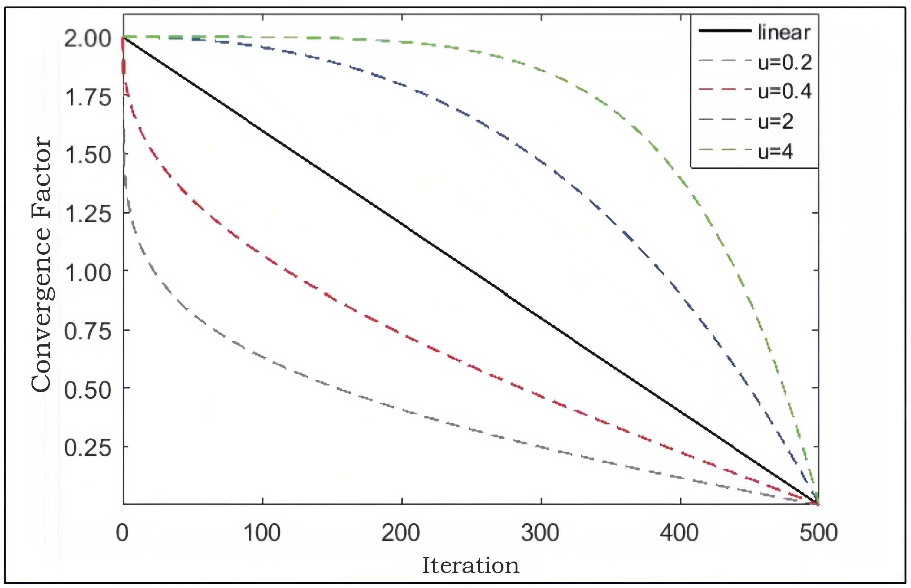
3.2.2. Nonlinear Convergence Factor and Adaptive Weight Coefficient
3.2.3. Multilevel Thresholding Using MSWOA
4. Performance Evaluation
4.1. Parameter Settings
4.2. Experimental Results and Analysis
5. Multilevel Image Thresholding Based on MSWOA
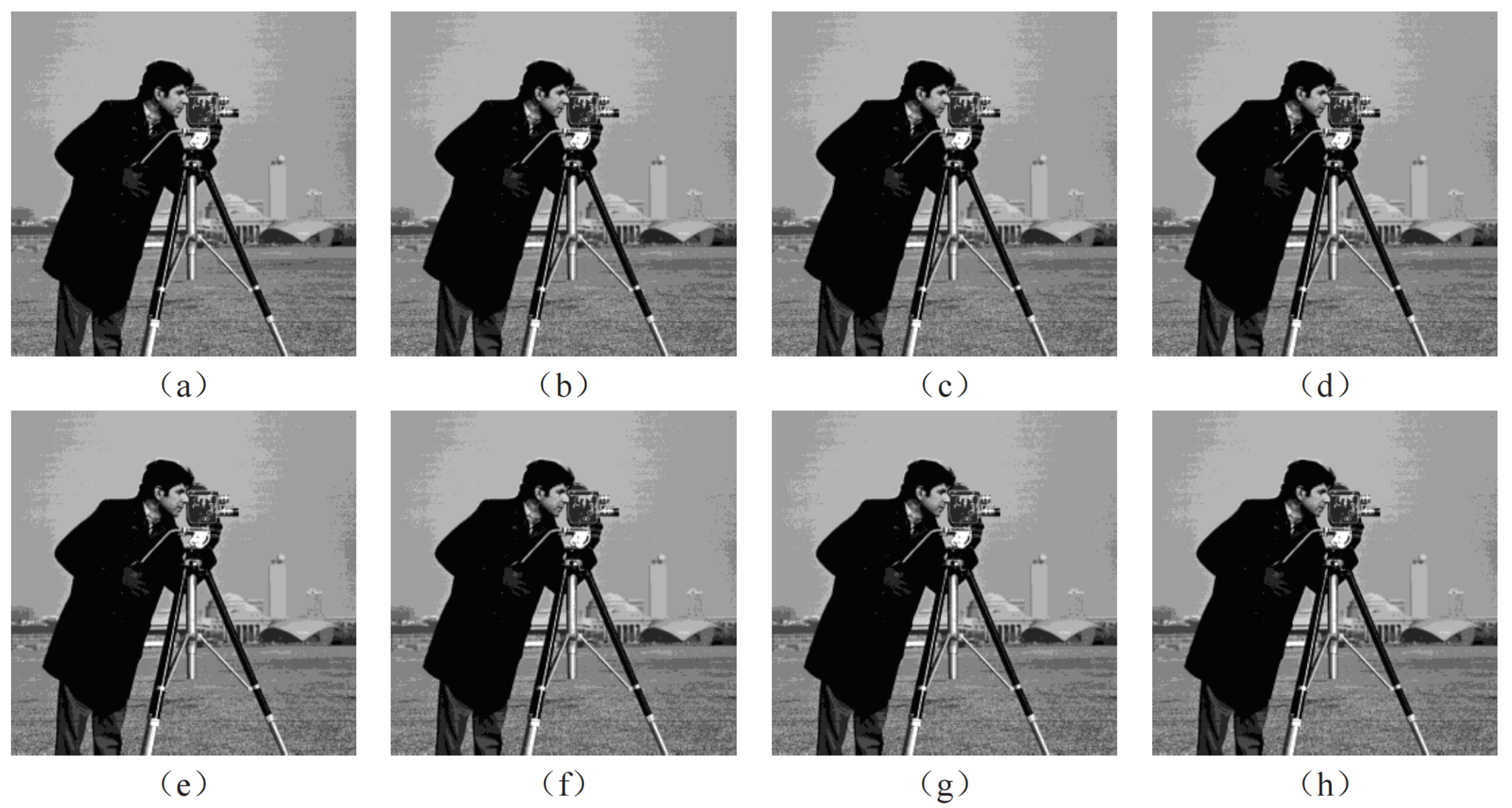
5.1. Benchmark Images
5.2. Experimental Settings
5.3. Segmented Image Quality Metrics
5.4. Experimental Results and Analysis
5.4.1. Analysis of Otsu and Kapur Methods
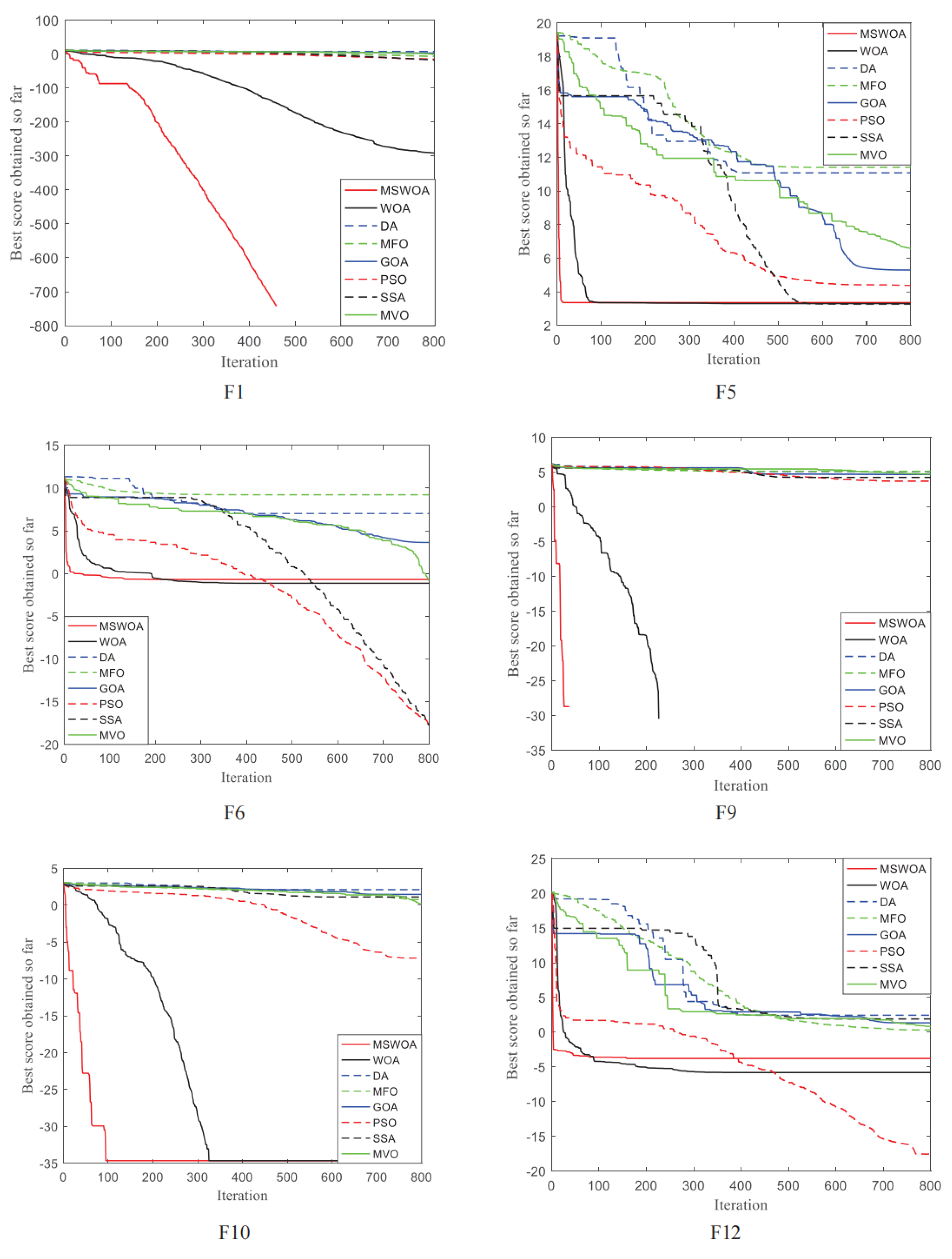
5.4.2. Analysis of MSWOA and Other Seven Optimization Algorithms
5.4.3. Statistical Analysis with Wilcoxon Rank Sum Test
6. Conclusions and Future Work
Author Contributions
Funding
Data Availability Statement
Acknowledgments
Conflicts of Interest
References
- Yan, L.; Li, K.; Gao, R.; Wang, C.; Xiong, N. An Intelligent Weighted Object Detector for Feature Extraction to Enrich Global Image Information. Appl. Sci. 2022, 12, 7825. [Google Scholar] [CrossRef]
- Yan, L.; Fu, J.; Wang, C.; Ye, Z.; Chen, H.; Ling, H. Enhanced network optimized generative adversarial network for image enhancement. Multimed. Tools Appl. 2021, 80, 14363–14381. [Google Scholar] [CrossRef]
- Yan, L.; Sheng, M.; Wang, C.; Gao, R.; Yu, H. Hybrid neural networks based facial expression recognition for smart city. Multimed. Tools Appl. 2022, 81, 319–342. [Google Scholar] [CrossRef]
- Wu, C.; Luo, C.; Xiong, N.; Zhang, W.; Kim, T.H. A greedy deep learning method for medical disease analysis. IEEE Access 2018, 6, 20021–20030. [Google Scholar] [CrossRef]
- Li, L.; Qian, B.; Lian, J.; Zheng, W.; Zhou, Y. Traffic scene segmentation based on RGB-D image and deep learning. IEEE Trans. Intell. Transp. Syst. 2017, 19, 1664–1669. [Google Scholar] [CrossRef]
- Kotaridis, I.; Lazaridou, M. Remote sensing image segmentation advances: A meta-analysis. ISPRS J. Photogramm. Remote Sens. 2021, 173, 309–322. [Google Scholar] [CrossRef]
- Jia, H.; Lang, C.; Oliva, D.; Song, W.; Peng, X. Dynamic harris hawks optimization with mutation mechanism for satellite image segmentation. Remote Sens. 2019, 11, 1421. [Google Scholar] [CrossRef] [Green Version]
- Shaikh, S.H.; Saeed, K.; Chaki, N.; Shaikh, S.H.; Saeed, K.; Chaki, N. Moving Object Detection Using Background Subtraction; Springer: Berlin/Heidelberg, Germany, 2014. [Google Scholar]
- Sharma, T.; Singh, H. Computational approach to image segmentation analysis. Int. J. Mod. Educ. Comput. Sci. 2017, 9, 30. [Google Scholar]
- Otsu, N. A threshold selection method from gray-level histograms. IEEE Trans. Syst. Man, Cybern. 1979, 9, 62–66. [Google Scholar] [CrossRef] [Green Version]
- Kapur, J.N.; Sahoo, P.K.; Wong, A.K. A new method for gray-level picture thresholding using the entropy of the histogram. Comput. Vision, Graph. Image Process. 1985, 29, 273–285. [Google Scholar] [CrossRef]
- Khairuzzaman, A.K.M.; Chaudhury, S. Brain MR image multilevel thresholding by using particle swarm optimization, Otsu method and anisotropic diffusion. Int. J. Appl. Metaheuristic Comput. 2019, 10, 91–106. [Google Scholar] [CrossRef] [Green Version]
- Gao, H.; Fu, Z.; Pun, C.M.; Hu, H.; Lan, R. A multi-level thresholding image segmentation based on an improved artificial bee colony algorithm. Comput. Electr. Eng. 2018, 70, 931–938. [Google Scholar] [CrossRef]
- Yue, X.; Zhang, H. Modified hybrid bat algorithm with genetic crossover operation and smart inertia weight for multilevel image segmentation. Appl. Soft Comput. 2020, 90, 106157. [Google Scholar] [CrossRef]
- Mirjalili, S. Moth-flame optimization algorithm: A novel nature-inspired heuristic paradigm. Knowl.-Based Syst. 2015, 89, 228–249. [Google Scholar] [CrossRef]
- Pare, S.; Kumar, A.; Bajaj, V.; Singh, G.K. A multilevel color image segmentation technique based on cuckoo search algorithm and energy curve. Appl. Soft Comput. 2016, 47, 76–102. [Google Scholar] [CrossRef]
- Bakhshali, M.A.; Shamsi, M. Segmentation of color lip images by optimal thresholding using bacterial foraging optimization (BFO). J. Comput. Sci. 2014, 5, 251–257. [Google Scholar] [CrossRef]
- Khairuzzaman, A.K.M.; Chaudhury, S. Multilevel thresholding using grey wolf optimizer for image segmentation. Expert Syst. Appl. 2017, 86, 64–76. [Google Scholar] [CrossRef]
- Chao, Y.; Dai, M.; Chen, K.; Chen, P.; Zhang, Z.S. Image segmentation of multilevel threshold using hybrid PSOGSA with generalized opposition-based learning. Guangxue Jingmi Gongcheng/Optics Precis. Eng. 2015, 23, 879–886. [Google Scholar]
- Agarwal, P.; Singh, R.; Kumar, S.; Bhattacharya, M. Social spider algorithm employed multi-level thresholding segmentation approach. In Proceedings of First International Conference on Information and Communication Technology for Intelligent Systems: Volume 2; Springer: Berlin/Heidelberg, Germany, 2016; pp. 249–259. [Google Scholar]
- Zhou, Y.; Yang, X.; Ling, Y.; Zhang, J. Meta-heuristic moth swarm algorithm for multilevel thresholding image segmentation. Multimed. Tools Appl. 2018, 77, 23699–23727. [Google Scholar] [CrossRef]
- Bhandari, A.K.; Rahul, K. A context sensitive Masi entropy for multilevel image segmentation using moth swarm algorithm. Infrared Phys. Technol. 2019, 98, 132–154. [Google Scholar] [CrossRef]
- Kapoor, S.; Zeya, I.; Singhal, C.; Nanda, S.J. A grey wolf optimizer based automatic clustering algorithm for satellite image segmentation. Procedia Comput. Sci. 2017, 115, 415–422. [Google Scholar] [CrossRef]
- Resma, K.B.; Nair, M.S. Multilevel thresholding for image segmentation using Krill Herd Optimization algorithm. J. King Saud Univ.-Comput. Inform. Sci. 2021, 33, 528–541. [Google Scholar]
- He, L.; Huang, S. An efficient krill herd algorithm for color image multilevel thresholding segmentation problem. Appl. Soft Comput. 2020, 89, 106063. [Google Scholar] [CrossRef]
- Ding, G.; Dong, F.; Zou, H. Fruit fly optimization algorithm based on a hybrid adaptive-cooperative learning and its application in multilevel image thresholding. Appl. Soft Comput. 2019, 84, 105704. [Google Scholar] [CrossRef]
- Upadhyay, P.; Chhabra, J.K. Kapur’s entropy based optimal multilevel image segmentation using crow search algorithm. Appl. Soft Comput. 2020, 97, 105522. [Google Scholar] [CrossRef]
- Xing, Z. An improved emperor penguin optimization based multilevel thresholding for color image segmentation. Knowl.-Based Syst. 2020, 194, 105570. [Google Scholar] [CrossRef]
- Rodríguez-Esparza, E.; Zanella-Calzada, L.A.; Oliva, D.; Heidari, A.A.; Zaldivar, D.; Pérez-Cisneros, M.; Foong, L.K. An efficient Harris hawks-inspired image segmentation method. Expert Syst. Appl. 2020, 155, 113428. [Google Scholar] [CrossRef]
- Wunnava, A.; Naik, M.K.; Panda, R.; Jena, B.; Abraham, A. An adaptive Harris hawks optimization technique for two dimensional grey gradient based multilevel image thresholding. Appl. Soft Comput. 2020, 95, 106526. [Google Scholar] [CrossRef]
- Abd Elaziz, M.; Heidari, A.A.; Fujita, H.; Moayedi, H. A competitive chain-based Harris Hawks Optimizer for global optimization and multi-level image thresholding problems. Appl. Soft Comput. 2020, 95, 106347. [Google Scholar] [CrossRef]
- Liu, Q.; Li, N.; Jia, H.; Qi, Q.; Abualigah, L. Modified remora optimization algorithm for global optimization and multilevel thresholding image segmentation. Mathematics 2022, 10, 1014. [Google Scholar] [CrossRef]
- Mirjalili, S.; Lewis, A. The Whale Optimization Algorithm. Adv. Eng. Softw. 2016, 95, 51–67. [Google Scholar] [CrossRef]
- Chen, H.; Xu, Y.; Wang, M.; Zhao, X. A Balanced Whale Optimization Algorithm for Constrained Engineering Design Problems. Appl. Math. Model. 2019, 71, 45–59. [Google Scholar] [CrossRef]
- Gharehchopogh, S. A comprehensive survey: Whale Optimization Algorithm and its applications. Swarm Evol. Comput. 2019, 48, 1–24. [Google Scholar] [CrossRef]
- Got, A.; Moussaoui, A.; Zouache, D. A guided population archive whale optimization algorithm for solving multiobjective optimization problems. Expert Syst. Appl. 2020, 141, 112972.1–112972.15. [Google Scholar] [CrossRef]
- Sun, Y.; Wang, X.; Chen, Y.; Liu, Z. A modified whale optimization algorithm for large-scale global optimization problems. Expert Syst. Appl. 2018, 114, 563–577. [Google Scholar] [CrossRef]
- Sun, Y.; Yang, T.; Liu, Z. A whale optimization algorithm based on quadratic interpolation for high-dimensional global optimization problems. Appl. Soft Comput. 2019, 85, 105744. [Google Scholar] [CrossRef]
- Petrovi, M.; Miljkovi, Z.; Jokić, A. A novel methodology for optimal single mobile robot scheduling using whale optimization algorithm—ScienceDirect. Applied Soft Comput. 2019, 81, 105520. [Google Scholar] [CrossRef]
- Abdel-Basset, M.; El-Shahat, D.; Deb, K.; Abouhawwash, M. Energy-aware whale optimization algorithm for real-time task scheduling in multiprocessor systems. Appl. Soft Comput. 2020, 93, 106349. [Google Scholar] [CrossRef]
- Li, H.; Ke, S.; Rao, X.; Li, C.; Chen, D.; Kuang, F.; Chen, H.; Liang, G.; Liu, L. An Improved Whale Optimizer with Multiple Strategies for Intelligent Prediction of Talent Stability. Electronics 2022, 11, 4224. [Google Scholar] [CrossRef]
- Abd El Aziz, M.; Ewees, A.A.; Hassanien, A.E. Whale optimization algorithm and moth-flame optimization for multilevel thresholding image segmentation. Expert Syst. Appl. 2017, 83, 242–256. [Google Scholar] [CrossRef]
- Zhang, Y.; Chen, F. An improved whale optimization algorithm. Comput. Eng. 2018, 44, 208–213+219. [Google Scholar]
- Mostafa Bozorgi, S.; Yazdani, S. IWOA: An improved whale optimization algorithm for optimization problems. J. Comput. Des. Eng. 2019, 6, 243–259. [Google Scholar] [CrossRef]
- Haupt, R.L.; Haupt, S.E. Practical Genetic Algorithms; John Wiley & Sons: Hoboken, NJ, USA, 2004. [Google Scholar]
- Gondro, C.; Kinghorn, B.P. A simple genetic algorithm for multiple sequence alignment. Genet. Mol. Res. 2007, 6, 964–982. [Google Scholar]
- Tizhoosh, H.R. Opposition-based learning: A new scheme for machine intelligence. In Proceedings of the International Conference on Computational Intelligence for Modelling, Control and Automation and International Conference on Intelligent Agents, Web Technologies and Internet Commerce (CIMCA-IAWTIC’06), Vienna, Austria, 28–30 November 2005; IEEE: New York, NY, USA, 2005; Volume 1, pp. 695–701. [Google Scholar]
- Mirjalili, S.; Gandomi, A.H.; Mirjalili, S.Z.; Saremi, S.; Faris, H.; Mirjalili, S.M. Salp Swarm Algorithm: A bio-inspired optimizer for engineering design problems. Adv. Eng. Softw. 2017, 114, 163–191. [Google Scholar] [CrossRef]
- Saremi, S.; Mirjalili, S.; Lewis, A. Grasshopper optimisation algorithm: Theory and application. Adv. Eng. Softw. 2017, 105, 30–47. [Google Scholar] [CrossRef] [Green Version]
- Mirjalili, S.; Mirjalili, S.M.; Hatamlou, A. Multi-verse optimizer: A nature-inspired algorithm for global optimization. Neural Comput. Appl. 2016, 27, 495–513. [Google Scholar] [CrossRef]
- Mirjalili, S. Dragonfly algorithm: A new meta-heuristic optimization technique for solving single-objective, discrete, and multi-objective problems. Neural Comput. Appl. 2016, 27, 1053–1073. [Google Scholar] [CrossRef]
- Wang, Z.; Bovik, A.C.; Sheikh, H.R.; Simoncelli, E.P. Image quality assessment: From error visibility to structural similarity. IEEE Trans. Image Process. 2004, 13, 600–612. [Google Scholar] [CrossRef] [Green Version]
- Patra, S.; Gautam, R.; Singla, A. A novel context sensitive multilevel thresholding for image segmentation. Appl. Soft Comput. 2014, 23, 122–127. [Google Scholar] [CrossRef]
- Kandhway, P.; Bhandari, A.K. Spatial context-based optimal multilevel energy curve thresholding for image segmentation using soft computing techniques. Neural Comput. Appl. 2020, 32, 8901–8937. [Google Scholar] [CrossRef]
- Dhiman, G.; Kumar, V. Seagull optimization algorithm: Theory and its applications for large-scale industrial engineering problems. Knowl.-Based Syst. 2019, 165, 169–196. [Google Scholar] [CrossRef]


| Function | Dim | Range | Type | |
|---|---|---|---|---|
| 30 | [−100, 100] | 0 | Unimodal | |
| 30 | [−10, 10] | 0 | Unimodal | |
| 30 | [−100, 100] | 0 | Unimodal | |
| 30 | [−100, 100] | 0 | Unimodal | |
| 30 | [−30, 30] | 0 | Unimodal | |
| 30 | [−100, 100] | 0 | Unimodal | |
| 30 | [−1.28, 1.28] | 0 | Unimodal | |
| 30 | [−500, 500] | Multimodal | ||
| 30 | [−5.12, 5.12] | 0 | Multimodal | |
| 30 | [−32, 32] | 0 | Multimodal | |
| 30 | [−600, 600] | 0 | Multimodal | |
| 30 | [−50, 50] | 0 | Multimodal | |
| 30 | [−50, 50] | 0 | Multimodal |
| Algorithm | Parameter | Value |
|---|---|---|
| MSWOA | u | 0.4 |
| WOA | Convergence factor a | |
| l | ||
| b | 1 | |
| PSO | Cognitive and social constants | |
| Inertial weigh | Linearly decreases from 0.9 to 0.2 | |
| SSA | nonlinearly decreases from 2 to 0 | |
| GOA | cmax | 1 |
| cmin | 0.00004 | |
| MFO | b | 1 |
| l | ||
| a | Linearly decreases from to | |
| MVO | 1 | |
| 0.2 | ||
| DA | f |
| F | MSWOA | WOA | PSO | SSA | GOA | MFO | MVO | DA | ||||||||
|---|---|---|---|---|---|---|---|---|---|---|---|---|---|---|---|---|
| Avg. | Std. | Avg. | Std. | Avg. | Std. | Avg. | Std. | Avg. | Std. | Avg. | Std. | Avg. | Std. | Avg. | Std. | |
| F1 | 0.00E+00 | 0.00E+00 | 5.68E-74 | 2.47E-73 | 1.14E-04 | 1.28E-04 | 1.94E-07 | 2.44E-07 | 3.88E+01 | 2.54E+01 | 2.68E+03 | 5.83E+03 | 2.68E+03 | 5.83E+03 | 2.73E+03 | 1.39E+03 |
| F2 | 2.18E-219 | 1.58E-219 | 2.85E-51 | 7.99E-51 | 7.31E-02 | 1.61E-01 | 1.71E+00 | 1.32E+00 | 1.82E+01 | 1.95E+01 | 2.91E+01 | 2.02E+01 | 2.91E+01 | 2.02E+01 | 1.65E+01 | 6.19E+00 |
| F3 | 0.00E+00 | 0.00E+00 | 4.32E+04 | 1.05E+04 | 7.36E+01 | 2.74E+01 | 2.14E+03 | 1.21E+03 | 3.36E+03 | 1.71E+03 | 1.57E+04 | 9.57E+03 | 1.57E+04 | 9.57E+03 | 1.32E+04 | 7.45E+03 |
| F4 | 2.48E-205 | 0.00E+00 | 4.89E+01 | 3.08E+01 | 1.11E+00 | 2.42E-01 | 1.22E+01 | 3.35E+00 | 1.39E+01 | 4.07E+00 | 6.81E+01 | 8.40E+00 | 6.81E+01 | 8.40E+00 | 3.14E+01 | 1.08E+01 |
| F5 | 2.76E+01 | 5.08E+00 | 2.79E+01 | 4.07E-01 | 9.62E+01 | 6.65E+01 | 2.59E+02 | 4.92E+02 | 6.60E+03 | 9.31E+03 | 1.42E+04 | 3.33E+04 | 1.42E+04 | 3.33E+04 | 2.46E+05 | 2.36E+05 |
| F6 | 4.04E-01 | 1.38E-01 | 4.40E-01 | 2.30E-01 | 2.01E-04 | 2.50E-04 | 9.92E-08 | 8.94E-08 | 3.73E+01 | 2.33E+01 | 3.68E+03 | 6.67E+03 | 3.68E+03 | 6.67E+03 | 2.42E+03 | 1.60E+03 |
| F7 | 6.88E-05 | 6.47E-05 | 3.51E-03 | 5.05E-03 | 1.61E-01 | 6.37E-02 | 1.99E-01 | 9.15E-02 | 5.08E-02 | 2.13E-02 | 2.07E+00 | 4.19E+00 | 2.07E+00 | 4.19E+00 | 6.89E-01 | 7.28E-01 |
| F8 | −1.25E+04 | 1.17E+02 | −9.89E+03 | 1.63E+03 | −4.82E+03 | 1.22E+03 | −7.47E+03 | 5.49E+02 | −7.30E+03 | 5.12E+02 | −8.66E+03 | 8.76E+02 | −8.66E+03 | 8.76E+02 | −5.35E+03 | 6.50E+02 |
| F9 | 0.00E+00 | 0.00E+00 | 0.00E+00 | 0.00E+00 | 5.53E+01 | 1.53E+01 | 6.08E+01 | 2.00E+01 | 1.03E+02 | 5.22E+01 | 1.62E+02 | 4.43E+01 | 1.62E+02 | 4.43E+01 | 1.69E+02 | 4.61E+01 |
| F10 | 8.88E-16 | 0.00E+00 | 5.03E-15 | 2.48E-15 | 2.29E-01 | 4.55E-01 | 2.70E+00 | 8.49E-01 | 5.65E+00 | 1.53E+00 | 1.43E+01 | 7.18E+00 | 1.43E+01 | 7.18E+00 | 1.01E+01 | 1.97E+00 |
| F11 | 0.00E+00 | 0.00E+00 | 2.02E-02 | 6.48E-02 | 8.05E-03 | 9.65E-03 | 2.02E-02 | 1.50E-02 | 1.15E+00 | 7.73E-02 | 1.13E+00 | 1.09E+00 | 1.13E+00 | 1.09E+00 | 1.73E+01 | 7.20E+00 |
| F12 | 2.19E-02 | 1.47E-02 | 2.12E-02 | 1.15E-02 | 3.12E-06 | 4.67E-06 | 9.04E+00 | 5.79E+00 | 1.11E+01 | 6.63E+00 | 8.59E+00 | 9.46E+00 | 8.59E+00 | 9.46E+00 | 3.06E+04 | 1.53E+05 |
| F13 | 3.01E-01 | 1.51E-01 | 4.67E-01 | 2.42E-01 | 7.38E-03 | 1.27E-02 | 1.83E+01 | 1.51E+01 | 4.15E+01 | 2.43E+01 | 1.37E+07 | 7.49E+07 | 1.37E+07 | 7.49E+07 | 2.75E+05 | 4.14E+05 |
| F | MSWOA | WOA | PSO | SSA | GOA | MFO | MVO | DA | ||||||||
|---|---|---|---|---|---|---|---|---|---|---|---|---|---|---|---|---|
| Avg. | Std. | Avg. | Std. | Avg. | Std. | Avg. | Std. | Avg. | Std. | Avg. | Std. | Avg. | Std. | Avg. | Std. | |
| F1 | 0.00E+00 | 0.00E+00 | 8.88E-120 | 4.54E-119 | 3.20E-06 | 1.21E-05 | 1.53E-08 | 3.79E-09 | 1.36E+01 | 1.15E+01 | 3.33E+02 | 1.83E+03 | 3.33E+02 | 1.83E+03 | 1.38E+03 | 7.31E+02 |
| F2 | 0.00E+00 | 0.00E+00 | 1.77E-83 | 5.71E-83 | 1.45E-03 | 1.76E-03 | 1.53E+00 | 1.34E+00 | 1.62E+01 | 2.58E+01 | 3.70E+01 | 1.88E+01 | 3.70E+01 | 1.88E+01 | 1.73E+01 | 7.80E+00 |
| F3 | 0.00E+00 | 0.00E+00 | 3.01E+04 | 1.31E+04 | 2.61E+01 | 9.84E+00 | 6.41E+02 | 4.62E+02 | 2.72E+03 | 1.47E+03 | 2.25E+04 | 1.78E+04 | 2.25E+04 | 1.78E+04 | 1.07E+04 | 6.00E+03 |
| F4 | 0.00E+00 | 0.00E+00 | 3.77E+01 | 3.16E+01 | 7.26E-01 | 2.09E-01 | 9.20E+00 | 4.01E+00 | 1.38E+01 | 3.81E+00 | 6.54E+01 | 9.36E+00 | 6.54E+01 | 9.36E+00 | 2.77E+01 | 9.06E+00 |
| F5 | 2.74E+01 | 5.07E+00 | 2.77E+01 | 5.08E-01 | 5.65E+01 | 4.64E+01 | 9.81E+01 | 1.26E+02 | 2.83E+03 | 4.98E+03 | 1.28E+04 | 3.09E+04 | 1.28E+04 | 3.09E+04 | 2.69E+05 | 3.48E+05 |
| F6 | 2.83E-01 | 1.15E-01 | 1.65E-01 | 1.21E-01 | 1.71E-06 | 8.05E-06 | 1.81E-08 | 5.81E-09 | 1.17E+01 | 8.30E+00 | 2.34E+03 | 4.32E+03 | 2.34E+03 | 4.32E+03 | 1.38E+03 | 7.37E+02 |
| F7 | 3.86E-05 | 3.29E-05 | 2.06E-03 | 3.69E-03 | 1.03E-01 | 4.20E-02 | 1.13E-01 | 3.82E-02 | 2.67E-02 | 1.21E-02 | 4.81E+00 | 6.84E+00 | 4.81E+00 | 6.84E+00 | 3.92E-01 | 2.74E-01 |
| F8 | −1.26E+04 | 1.14E+00 | −1.07E+04 | 1.75E+03 | −5.95E+03 | 1.31E+03 | −7.36E+03 | 8.10E+02 | −7.52E+03 | 7.54E+02 | −8.67E+03 | 9.27E+02 | −8.67E+03 | 9.27E+02 | −5.47E+03 | 6.24E+02 |
| F9 | 0.00E+00 | 0.00E+00 | 0.00E+00 | 0.00E+00 | 4.82E+01 | 1.27E+01 | 5.62E+01 | 1.60E+01 | 1.02E+02 | 3.64E+01 | 1.55E+02 | 4.04E+01 | 1.55E+02 | 4.04E+01 | 1.62E+02 | 3.29E+01 |
| F10 | 8.88E-16 | 0.00E+00 | 3.61E-15 | 2.41E-15 | 1.37E-01 | 4.26E-01 | 2.35E+00 | 4.92E-01 | 4.55E+00 | 1.13E+00 | 1.41E+01 | 7.19E+00 | 1.41E+01 | 7.19E+00 | 9.16E+00 | 1.70E+00 |
| F11 | 0.00E+00 | 0.00E+00 | 1.79E-02 | 5.81E-02 | 1.55E-01 | 8.85E-03 | 8.04E-03 | 8.04E-03 | 8.77E-01 | 1.55E-01 | 1.51E+01 | 4.15E+01 | 1.51E+01 | 4.15E+01 | 1.32E+01 | 5.95E+00 |
| F12 | 1.59E-02 | 1.06E-02 | 1.38E-02 | 1.88E-02 | 6.99E-09 | 1.66E-08 | 5.03E+00 | 2.90E+00 | 8.22E+00 | 5.74E+00 | 1.47E+00 | 1.49E+00 | 1.47E+00 | 1.49E+00 | 5.44E+01 | 1.28E+02 |
| F13 | 2.30E-01 | 9.58E-02 | 3.17E-01 | 2.25E-01 | 2.93E-03 | 4.94E-03 | 7.53E+00 | 1.57E+01 | 2.76E+01 | 1.57E+01 | 4.24E+00 | 6.60E+00 | 4.24E+00 | 6.60E+00 | 1.15E+05 | 2.62E+05 |
| Image | m | MSWOA | WOA | PSO | SSA | GOA | MFO | MVO | DA | ||||||||
|---|---|---|---|---|---|---|---|---|---|---|---|---|---|---|---|---|---|
| Otsu | Kapur | Otsu | Kapur | Otsu | Kapur | Otsu | Kapur | Otsu | Kapur | Otsu | Kapur | Otsu | Kapur | Otsu | Kapur | ||
| Lena | 2 | 11.9025 | 14.4845 | 11.9025 | 14.3883 | 11.9025 | 14.3883 | 11.9025 | 14.3883 | 11.9025 | 14.3883 | 11.9025 | 14.3883 | 11.9025 | 14.3883 | 11.9025 | 14.3883 |
| 3 | 14.1027 | 16.9552 | 14.1027 | 16.8255 | 14.1027 | 16.8255 | 14.1027 | 16.8255 | 13.7579 | 16.3516 | 14.1027 | 16.8481 | 14.1027 | 16.8255 | 14.1027 | 16.8255 | |
| 5 | 19.2113 | 19.8729 | 19.1614 | 19.7923 | 16.9648 | 19.7923 | 16.9648 | 19.7923 | 18.9844 | 19.7882 | 17.2025 | 19.8662 | 16.9648 | 19.7923 | 16.9648 | 19.8662 | |
| 8 | 22.5797 | 24.9741 | 20.5756 | 21.8269 | 19.9752 | 22.7018 | 20.7126 | 22.7093 | 20.3216 | 22.7085 | 20.3667 | 22.5234 | 20.3368 | 22.7083 | 20.4286 | 22.9321 | |
| Baboon | 2 | 11.5837 | 12.3381 | 11.5837 | 12.3381 | 11.5837 | 12.3381 | 11.5837 | 12.3381 | 11.5837 | 12.3381 | 11.5837 | 12.3381 | 11.5837 | 12.3381 | 11.5837 | 12.3381 |
| 3 | 13.6321 | 14.3441 | 13.5413 | 14.3441 | 13.5413 | 14.3441 | 13.5413 | 14.3441 | 13.3099 | 14.275 | 13.5413 | 14.3441 | 13.5413 | 14.3441 | 13.5413 | 14.3441 | |
| 5 | 17.1771 | 22.9336 | 17.2723 | 22.859 | 16.1728 | 22.8544 | 16.1728 | 22.8544 | 17.1589 | 21.6078 | 16.1728 | 22.859 | 16.1728 | 22.8544 | 16.1728 | 22.859 | |
| 8 | 20.3869 | 30.3807 | 20.018 | 30.3609 | 18.3586 | 30.2933 | 18.5683 | 30.2947 | 18.7169 | 30.3341 | 18.6087 | 30.3259 | 18.5668 | 30.3063 | 19.9064 | 30.3144 | |
| Starfish | 2 | 12.697 | 15.1602 | 12.6237 | 15.1602 | 12.6237 | 15.1602 | 12.6237 | 15.1602 | 12.6237 | 15.1602 | 12.6237 | 15.1602 | 12.6237 | 15.1602 | 12.6237 | 15.1602 |
| 3 | 15.2587 | 18.1574 | 15.2587 | 18.1574 | 15.2587 | 18.1574 | 15.2587 | 18.1574 | 14.4788 | 17.7476 | 15.3654 | 18.1574 | 15.2587 | 18.1574 | 15.2691 | 18.1574 | |
| 5 | 19.59 | 22.2217 | 19.0518 | 22.0858 | 19.0518 | 21.971 | 19.0518 | 21.971 | 19.1947 | 22.1121 | 19.0518 | 22.0858 | 19.0518 | 21.971 | 19.0518 | 21.9724 | |
| 8 | 25.2279 | 28.3071 | 23.1711 | 25.2777 | 22.2434 | 25.3942 | 22.7858 | 25.3805 | 22.5893 | 25.4139 | 22.2528 | 25.7199 | 22.2434 | 25.1868 | 22.7135 | 25.3236 | |
| Couple | 2 | 12.1121 | 14.2889 | 12.1121 | 14.2889 | 12.1121 | 14.2889 | 12.1121 | 14.2889 | 12.1121 | 14.2889 | 12.1121 | 14.2889 | 12.1121 | 14.2889 | 12.1121 | 14.2889 |
| 3 | 14.2726 | 16.9785 | 14.2726 | 16.9265 | 14.2726 | 16.9265 | 14.2726 | 16.9265 | 17.5171 | 18.1743 | 14.2726 | 16.9265 | 14.2726 | 16.9265 | 14.2726 | 16.9265 | |
| 5 | 18.1173 | 20.7261 | 16.8914 | 20.5302 | 16.8914 | 20.4364 | 16.8914 | 20.4364 | 19.8416 | 21.9673 | 17.6576 | 20.4364 | 16.5569 | 20.4364 | 16.7982 | 20.5302 | |
| 8 | 25.3153 | 28.1138 | 20.7382 | 22.0762 | 19.919 | 22.0762 | 21.7495 | 22.0762 | 20.5679 | 22.0482 | 20.7138 | 22.0762 | 21.4869 | 22.0762 | 21.4539 | 22.241 | |
| Cameraman | 2 | 12.231 | 14.9016 | 12.231 | 14.729 | 12.231 | 14.729 | 12.231 | 14.729 | 12.231 | 14.729 | 12.231 | 14.729 | 12.231 | 14.729 | 12.231 | 14.729 |
| 3 | 15.7204 | 21.7574 | 14.5472 | 21.2833 | 14.5472 | 21.2833 | 14.5472 | 21.2833 | 13.7709 | 21.0183 | 14.5472 | 21.418 | 14.5472 | 21.2833 | 14.5472 | 21.2833 | |
| 5 | 18.6227 | 26.0676 | 18.6207 | 25.683 | 17.6339 | 25.8299 | 18.5595 | 25.6675 | 18.5093 | 25.3852 | 17.8744 | 25.8332 | 18.4315 | 25.6675 | 18.5271 | 25.6894 | |
| 8 | 20.993 | 29.1303 | 20.8943 | 29.0543 | 20.6932 | 29.0267 | 20.81 | 29.0267 | 20.8285 | 29.0265 | 20.6976 | 29.0454 | 20.8618 | 28.9892 | 23.9218 | 29.0309 | |
| Pepper | 2 | 12.2981 | 13.211 | 12.2981 | 13.211 | 12.2981 | 13.211 | 12.2981 | 13.211 | 12.2981 | 13.211 | 12.2981 | 13.211 | 12.2981 | 13.211 | 12.2981 | 13.211 |
| 3 | 14.4837 | 15.4188 | 14.4082 | 15.4188 | 14.4082 | 15.4188 | 14.4082 | 15.4188 | 14.4124 | 13.6771 | 14.4082 | 15.4188 | 14.4082 | 15.4188 | 14.4082 | 15.4188 | |
| 5 | 19.5722 | 23.561 | 18.0195 | 23.3721 | 16.7909 | 23.2099 | 16.8888 | 23.2099 | 18.3362 | 21.7569 | 17.1978 | 23.3058 | 17.1978 | 23.2099 | 17.1978 | 23.2954 | |
| 8 | 22.7276 | 29.5103 | 22.3483 | 29.3608 | 20.1303 | 27.5703 | 21.9444 | 28.5212 | 20.4323 | 28.6622 | 20.1355 | 28.8707 | 20.2841 | 28.5367 | 20.1161 | 29.0532 | |
| Tree | 2 | 13.9934 | 16.5731 | 13.9934 | 16.4114 | 13.9934 | 16.4114 | 13.9934 | 16.4114 | 13.9934 | 16.4114 | 13.9934 | 16.4114 | 13.9934 | 16.4114 | 13.9934 | 16.4114 |
| 3 | 16.7393 | 19.8968 | 16.5091 | 19.7753 | 16.5091 | 19.7753 | 16.5091 | 19.7753 | 15.968 | 20.5578 | 16.5091 | 19.7753 | 16.5091 | 19.7753 | 16.5091 | 19.8155 | |
| 5 | 21.3783 | 22.5034 | 20.0391 | 22.1753 | 19.8873 | 22.4102 | 19.9665 | 22.141 | 20.1136 | 21.6881 | 20.0394 | 22.4102 | 20.0075 | 22.141 | 19.9486 | 22.2266 | |
| 8 | 25.4625 | 28.3796 | 25.0236 | 26.0232 | 23.5182 | 25.5521 | 24.418 | 25.5543 | 24.3086 | 25.5089 | 24.233 | 25.5654 | 24.437 | 25.3931 | 25.5159 | 25.6348 | |
| Building | 2 | 12.0557 | 12.1508 | 12.0557 | 12.1508 | 12.0557 | 12.1508 | 12.0557 | 12.1508 | 12.0557 | 12.1508 | 12.0557 | 12.1508 | 12.0557 | 12.1508 | 12.0557 | 12.1508 |
| 3 | 14.0772 | 13.4318 | 13.9276 | 13.4318 | 13.9276 | 13.4318 | 13.9276 | 13.4318 | 13.6812 | 12.7967 | 13.9276 | 13.4318 | 13.9276 | 13.4318 | 13.9276 | 13.4318 | |
| 5 | 18.4052 | 19.2348 | 17.7485 | 19.2325 | 16.5801 | 19.2325 | 16.5801 | 19.2325 | 18.3092 | 22.1147 | 16.5801 | 19.2325 | 16.5801 | 19.2325 | 17.3635 | 19.2325 | |
| 8 | 20.9671 | 30.3721 | 20.8138 | 29.8267 | 18.2647 | 28.1713 | 20.1842 | 28.1738 | 18.5888 | 28.3911 | 18.466 | 28.1801 | 18.2695 | 28.1713 | 19.6706 | 28.7902 | |
| Image | m | MSWOA | WOA | PSO | SSA | GOA | MFO | MVO | DA | ||||||||
|---|---|---|---|---|---|---|---|---|---|---|---|---|---|---|---|---|---|
| Otsu | Kapur | Otsu | Kapur | Otsu | Kapur | Otsu | Kapur | Otsu | Kapur | Otsu | Kapur | Otsu | Kapur | Otsu | Kapur | ||
| Lena | 2 | 0.38469 | 0.48354 | 0.38469 | 0.47856 | 0.38469 | 0.47856 | 0.38469 | 0.47856 | 0.38469 | 0.47856 | 0.38469 | 0.47856 | 0.38469 | 0.47856 | 0.38469 | 0.47856 |
| 3 | 0.46863 | 0.57261 | 0.46863 | 0.5661 | 0.46863 | 0.5661 | 0.46863 | 0.5661 | 0.53953 | 0.5747 | 0.46863 | 0.56327 | 0.46863 | 0.5661 | 0.46863 | 0.5661 | |
| 5 | 0.70299 | 0.64855 | 0.69893 | 0.65079 | 0.5953 | 0.65079 | 0.5953 | 0.65079 | 0.65574 | 0.64961 | 0.61027 | 0.65061 | 0.5953 | 0.65079 | 0.5953 | 0.65061 | |
| 8 | 0.80157 | 0.78909 | 0.72308 | 0.72653 | 0.70873 | 0.72556 | 0.72737 | 0.725 | 0.71318 | 0.72993 | 0.71964 | 0.72535 | 0.71622 | 0.72484 | 0.7153 | 0.7316 | |
| Baboon | 2 | 0.44418 | 0.51738 | 0.44418 | 0.51738 | 0.44418 | 0.51738 | 0.44418 | 0.51738 | 0.44418 | 0.51738 | 0.44418 | 0.51738 | 0.44418 | 0.51738 | 0.44418 | 0.51738 |
| 3 | 0.52143 | 0.62295 | 0.52115 | 0.62295 | 0.52115 | 0.62295 | 0.52115 | 0.62295 | 0.56317 | 0.61809 | 0.52115 | 0.62295 | 0.52115 | 0.62295 | 0.52115 | 0.62295 | |
| 5 | 0.70501 | 0.79125 | 0.71025 | 0.79012 | 0.64116 | 0.78958 | 0.64116 | 0.78958 | 0.67826 | 0.77005 | 0.64116 | 0.79012 | 0.64116 | 0.78958 | 0.64116 | 0.79012 | |
| 8 | 0.80349 | 0.90719 | 0.80074 | 0.90603 | 0.7261 | 0.90579 | 0.73494 | 0.90583 | 0.73576 | 0.90605 | 0.72769 | 0.90644 | 0.7349 | 0.90598 | 0.75196 | 0.90688 | |
| Starfish | 2 | 0.32402 | 0.37677 | 0.31997 | 0.37677 | 0.31997 | 0.37677 | 0.31997 | 0.37677 | 0.31997 | 0.37677 | 0.31997 | 0.37677 | 0.31997 | 0.37677 | 0.31997 | 0.37677 |
| 3 | 0.44135 | 0.50411 | 0.44135 | 0.50411 | 0.44135 | 0.50411 | 0.44135 | 0.50411 | 0.44856 | 0.53117 | 0.44372 | 0.50411 | 0.44135 | 0.50411 | 0.43892 | 0.50411 | |
| 5 | 0.6384 | 0.65176 | 0.61666 | 0.65019 | 0.61666 | 0.64842 | 0.61666 | 0.64842 | 0.6172 | 0.6669 | 0.61666 | 0.65019 | 0.61666 | 0.64842 | 0.61666 | 0.64841 | |
| 8 | 0.85447 | 0.84501 | 0.75891 | 0.76051 | 0.73528 | 0.76604 | 0.74951 | 0.76902 | 0.75064 | 0.76787 | 0.73579 | 0.77422 | 0.73528 | 0.76435 | 0.72405 | 0.76448 | |
| Couple | 2 | 0.42424 | 0.48148 | 0.42424 | 0.48148 | 0.42424 | 0.48148 | 0.42424 | 0.48148 | 0.42424 | 0.48148 | 0.42424 | 0.48148 | 0.42424 | 0.48148 | 0.42424 | 0.48148 |
| 3 | 0.5046 | 0.57505 | 0.5046 | 0.57523 | 0.5046 | 0.57523 | 0.5046 | 0.57523 | 0.63914 | 0.60493 | 0.5046 | 0.57523 | 0.5046 | 0.57523 | 0.5046 | 0.57523 | |
| 5 | 0.65832 | 0.69971 | 0.62697 | 0.69618 | 0.62697 | 0.69469 | 0.62697 | 0.69469 | 0.68041 | 0.71734 | 0.64438 | 0.69469 | 0.61397 | 0.69469 | 0.62153 | 0.69618 | |
| 8 | 0.83363 | 0.85812 | 0.74142 | 0.77094 | 0.73274 | 0.77094 | 0.756 | 0.77094 | 0.74062 | 0.76977 | 0.74641 | 0.77094 | 0.75415 | 0.77094 | 0.75271 | 0.77335 | |
| Cameraman | 2 | 0.4337 | 0.54566 | 0.4337 | 0.54219 | 0.4337 | 0.54219 | 0.4337 | 0.54219 | 0.4337 | 0.54219 | 0.4337 | 0.54219 | 0.4337 | 0.54219 | 0.4337 | 0.54219 |
| 3 | 0.52401 | 0.65435 | 0.48218 | 0.67089 | 0.48218 | 0.67089 | 0.48218 | 0.67089 | 0.58483 | 0.66203 | 0.48218 | 0.67177 | 0.48218 | 0.67089 | 0.48218 | 0.67089 | |
| 5 | 0.61409 | 0.72728 | 0.61366 | 0.7218 | 0.5838 | 0.72222 | 0.61256 | 0.72073 | 0.63054 | 0.72917 | 0.58382 | 0.72226 | 0.61194 | 0.72073 | 0.61261 | 0.7224 | |
| 8 | 0.67576 | 0.75398 | 0.6727 | 0.75446 | 0.66587 | 0.7536 | 0.66945 | 0.7536 | 0.66986 | 0.75109 | 0.6663 | 0.75356 | 0.67207 | 0.75146 | 0.72546 | 0.75374 | |
| Pepper | 2 | 0.37259 | 0.52509 | 0.37259 | 0.52509 | 0.37259 | 0.52509 | 0.37259 | 0.52509 | 0.37259 | 0.52509 | 0.37259 | 0.52509 | 0.37259 | 0.52509 | 0.37259 | 0.52509 |
| 3 | 0.47407 | 0.60368 | 0.4709 | 0.60368 | 0.4709 | 0.60368 | 0.4709 | 0.60368 | 0.54324 | 0.55867 | 0.4709 | 0.60368 | 0.4709 | 0.60368 | 0.4709 | 0.60368 | |
| 5 | 0.66539 | 0.73477 | 0.61695 | 0.72891 | 0.56822 | 0.7254 | 0.5663 | 0.7254 | 0.62583 | 0.67435 | 0.5894 | 0.7272 | 0.5894 | 0.7254 | 0.5894 | 0.72665 | |
| 8 | 0.76063 | 0.82785 | 0.76389 | 0.82146 | 0.6947 | 0.81031 | 0.74605 | 0.80994 | 0.69994 | 0.81331 | 0.69496 | 0.81627 | 0.69825 | 0.80977 | 0.69047 | 0.82057 | |
| Tree | 2 | 0.49566 | 0.51668 | 0.49566 | 0.51024 | 0.49566 | 0.51024 | 0.49566 | 0.51024 | 0.49566 | 0.51024 | 0.49566 | 0.51024 | 0.49566 | 0.51024 | 0.49566 | 0.51024 |
| 3 | 0.54613 | 0.63348 | 0.51989 | 0.62626 | 0.51989 | 0.62626 | 0.51989 | 0.62626 | 0.66417 | 0.70363 | 0.51989 | 0.62626 | 0.51989 | 0.62626 | 0.51989 | 0.62858 | |
| 5 | 0.67056 | 0.66774 | 0.64365 | 0.65768 | 0.62807 | 0.66891 | 0.64419 | 0.65534 | 0.65817 | 0.66971 | 0.63699 | 0.66891 | 0.64396 | 0.65534 | 0.6329 | 0.66488 | |
| 8 | 0.814 | 0.84406 | 0.79544 | 0.75482 | 0.73269 | 0.74323 | 0.74858 | 0.74279 | 0.73825 | 0.74241 | 0.75644 | 0.74248 | 0.79721 | 0.73817 | 0.75012 | 0.74028 | |
| Building | 2 | 0.35267 | 0.573 | 0.35267 | 0.573 | 0.35267 | 0.573 | 0.35267 | 0.573 | 0.35267 | 0.573 | 0.35267 | 0.573 | 0.35267 | 0.573 | 0.35267 | 0.573 |
| 3 | 0.47778 | 0.6141 | 0.4602 | 0.6141 | 0.4602 | 0.6141 | 0.4602 | 0.6141 | 0.46291 | 0.61332 | 0.4602 | 0.6141 | 0.4602 | 0.6141 | 0.4602 | 0.6141 | |
| 5 | 0.698 | 0.72373 | 0.68839 | 0.72254 | 0.59742 | 0.72254 | 0.59742 | 0.72254 | 0.68095 | 0.78525 | 0.59742 | 0.72254 | 0.59742 | 0.72254 | 0.62213 | 0.72254 | |
| 8 | 0.76008 | 0.91042 | 0.75812 | 0.89699 | 0.66833 | 0.88193 | 0.74163 | 0.88185 | 0.68433 | 0.88479 | 0.67421 | 0.87996 | 0.66962 | 0.88193 | 0.71373 | 0.88609 | |
| Image | m | MSWOA | WOA | PSO | SSA | GOA | MFO | MVO | DA | ||||||||
|---|---|---|---|---|---|---|---|---|---|---|---|---|---|---|---|---|---|
| Otsu | Kapur | Otsu | Kapur | Otsu | Kapur | Otsu | Kapur | Otsu | Kapur | Otsu | Kapur | Otsu | Kapur | Otsu | Kapur | ||
| Lena | 2 | 0.66709 | 0.68502 | 0.66709 | 0.68355 | 0.66709 | 0.68355 | 0.66709 | 0.68355 | 0.66709 | 0.68355 | 0.66709 | 0.68355 | 0.66709 | 0.68355 | 0.66709 | 0.68355 |
| 3 | 0.71461 | 0.75583 | 0.71461 | 0.75424 | 0.71461 | 0.75424 | 0.71461 | 0.75424 | 0.73591 | 0.74224 | 0.71461 | 0.75245 | 0.71461 | 0.75424 | 0.71461 | 0.75424 | |
| 5 | 0.80462 | 0.84361 | 0.80161 | 0.84327 | 0.8061 | 0.84327 | 0.8061 | 0.84327 | 0.8027 | 0.84442 | 0.81027 | 0.84135 | 0.8061 | 0.84327 | 0.8061 | 0.84135 | |
| 8 | 0.90754 | 0.90661 | 0.87568 | 0.88462 | 0.8802 | 0.89071 | 0.87403 | 0.89137 | 0.87887 | 0.89146 | 0.88062 | 0.8951 | 0.87778 | 0.89179 | 0.87737 | 0.88891 | |
| Baboon | 2 | 0.688 | 0.73346 | 0.688 | 0.73346 | 0.688 | 0.73346 | 0.688 | 0.73346 | 0.688 | 0.73346 | 0.688 | 0.73346 | 0.688 | 0.73346 | 0.688 | 0.73346 |
| 3 | 0.75093 | 0.79605 | 0.75005 | 0.79605 | 0.75005 | 0.79605 | 0.75005 | 0.79605 | 0.76046 | 0.79347 | 0.75005 | 0.79605 | 0.75005 | 0.79605 | 0.75005 | 0.79605 | |
| 5 | 0.81479 | 0.89807 | 0.8179 | 0.89676 | 0.80484 | 0.89663 | 0.80484 | 0.89663 | 0.82366 | 0.89796 | 0.80484 | 0.89676 | 0.80484 | 0.89663 | 0.80484 | 0.89676 | |
| 8 | 0.86657 | 0.97901 | 0.86399 | 0.97865 | 0.84049 | 0.97836 | 0.84382 | 0.97833 | 0.84615 | 0.97879 | 0.84562 | 0.97819 | 0.84386 | 0.97826 | 0.8932 | 0.97857 | |
| Starfish | 2 | 0.55442 | 0.57051 | 0.55295 | 0.57051 | 0.55295 | 0.57051 | 0.55295 | 0.57051 | 0.55295 | 0.57051 | 0.55295 | 0.57051 | 0.55295 | 0.57051 | 0.55295 | 0.57051 |
| 3 | 0.64086 | 0.66335 | 0.64086 | 0.66335 | 0.64086 | 0.66335 | 0.64086 | 0.66335 | 0.63624 | 0.66263 | 0.64228 | 0.66335 | 0.64086 | 0.66335 | 0.64022 | 0.66335 | |
| 5 | 0.77469 | 0.77491 | 0.76794 | 0.77584 | 0.76794 | 0.77618 | 0.76794 | 0.77618 | 0.76785 | 0.77394 | 0.76794 | 0.77584 | 0.76794 | 0.77618 | 0.76794 | 0.77644 | |
| 8 | 0.86523 | 0.86684 | 0.85618 | 0.85909 | 0.85164 | 0.86286 | 0.85582 | 0.86549 | 0.84919 | 0.8643 | 0.85235 | 0.86668 | 0.85164 | 0.86291 | 0.83965 | 0.86261 | |
| Couple | 2 | 0.62621 | 0.64581 | 0.62621 | 0.64581 | 0.62621 | 0.64581 | 0.62621 | 0.64581 | 0.62621 | 0.64581 | 0.62621 | 0.64581 | 0.62621 | 0.64581 | 0.62621 | 0.64581 |
| 3 | 0.69087 | 0.72318 | 0.69087 | 0.72336 | 0.69087 | 0.72336 | 0.69087 | 0.72336 | 0.68601 | 0.66714 | 0.69087 | 0.72336 | 0.69087 | 0.72336 | 0.69087 | 0.72336 | |
| 5 | 0.7896 | 0.81238 | 0.76813 | 0.81234 | 0.76813 | 0.8127 | 0.76813 | 0.8127 | 0.78228 | 0.77021 | 0.78754 | 0.8127 | 0.7604 | 0.8127 | 0.7648 | 0.81234 | |
| 8 | 0.8412 | 0.89005 | 0.84638 | 0.86496 | 0.84603 | 0.86496 | 0.83553 | 0.86496 | 0.84271 | 0.86409 | 0.84774 | 0.86496 | 0.83688 | 0.86496 | 0.83935 | 0.86422 | |
| Cameraman | 2 | 0.62811 | 0.65634 | 0.62811 | 0.65467 | 0.62811 | 0.65467 | 0.62811 | 0.65467 | 0.62811 | 0.65467 | 0.62811 | 0.65467 | 0.62811 | 0.65467 | 0.62811 | 0.65467 |
| 3 | 0.71029 | 0.78483 | 0.67558 | 0.79562 | 0.67558 | 0.79562 | 0.67558 | 0.79562 | 0.76263 | 0.79189 | 0.67558 | 0.79546 | 0.67558 | 0.79562 | 0.67558 | 0.79562 | |
| 5 | 0.79243 | 0.86897 | 0.79129 | 0.85491 | 0.7614 | 0.86627 | 0.78938 | 0.85596 | 0.80823 | 0.87304 | 0.75929 | 0.86623 | 0.78603 | 0.85596 | 0.78782 | 0.8592 | |
| 8 | 0.83747 | 0.90969 | 0.83611 | 0.91034 | 0.82432 | 0.9093 | 0.83093 | 0.9093 | 0.83006 | 0.90818 | 0.8259 | 0.90933 | 0.83586 | 0.90783 | 0.81813 | 0.90993 | |
| Pepper | 2 | 0.61103 | 0.64532 | 0.61103 | 0.64532 | 0.61103 | 0.64532 | 0.61103 | 0.64532 | 0.61103 | 0.64532 | 0.61103 | 0.64532 | 0.61103 | 0.64532 | 0.61103 | 0.64532 |
| 3 | 0.66632 | 0.7008 | 0.6662 | 0.7008 | 0.6662 | 0.7008 | 0.6662 | 0.7008 | 0.67632 | 0.68421 | 0.6662 | 0.7008 | 0.6662 | 0.7008 | 0.6662 | 0.7008 | |
| 5 | 0.77134 | 0.78993 | 0.75042 | 0.788 | 0.72792 | 0.78884 | 0.72539 | 0.78884 | 0.74203 | 0.76781 | 0.7357 | 0.78881 | 0.7357 | 0.78884 | 0.7357 | 0.78903 | |
| 8 | 0.81246 | 0.85776 | 0.80773 | 0.85752 | 0.79761 | 0.87135 | 0.82421 | 0.86303 | 0.79961 | 0.86398 | 0.7979 | 0.86285 | 0.79801 | 0.86332 | 0.79446 | 0.85741 | |
| Tree | 2 | 0.6901 | 0.69492 | 0.6901 | 0.6925 | 0.6901 | 0.6925 | 0.6901 | 0.6925 | 0.6901 | 0.6925 | 0.6901 | 0.6925 | 0.6901 | 0.6925 | 0.6901 | 0.6925 |
| 3 | 0.71442 | 0.7664 | 0.70264 | 0.7647 | 0.70264 | 0.7647 | 0.70264 | 0.7647 | 0.75091 | 0.78328 | 0.70264 | 0.7647 | 0.70264 | 0.7647 | 0.70264 | 0.76547 | |
| 5 | 0.79345 | 0.79837 | 0.77636 | 0.79379 | 0.77316 | 0.79648 | 0.77406 | 0.79364 | 0.7712 | 0.79678 | 0.77638 | 0.79648 | 0.77542 | 0.79364 | 0.77363 | 0.79743 | |
| 8 | 0.84685 | 0.86426 | 0.83214 | 0.85264 | 0.82945 | 0.84984 | 0.83514 | 0.84984 | 0.83549 | 0.8495 | 0.84328 | 0.84994 | 0.83332 | 0.84886 | 0.83778 | 0.84956 | |
| Building | 2 | 0.62024 | 0.60693 | 0.62024 | 0.60693 | 0.62024 | 0.60693 | 0.62024 | 0.60693 | 0.62024 | 0.60693 | 0.62024 | 0.60693 | 0.62024 | 0.60693 | 0.62024 | 0.60693 |
| 3 | 0.6793 | 0.65926 | 0.67837 | 0.65926 | 0.67837 | 0.65926 | 0.67837 | 0.65926 | 0.64477 | 0.64741 | 0.67837 | 0.65926 | 0.67837 | 0.65926 | 0.67837 | 0.65926 | |
| 5 | 0.74698 | 0.76923 | 0.73842 | 0.76816 | 0.73181 | 0.76816 | 0.73181 | 0.76816 | 0.76116 | 0.79763 | 0.73181 | 0.76816 | 0.73181 | 0.76816 | 0.77878 | 0.76816 | |
| 8 | 0.81805 | 0.90462 | 0.79738 | 0.90365 | 0.77242 | 0.90049 | 0.80183 | 0.90036 | 0.77753 | 0.9008 | 0.77692 | 0.90017 | 0.77327 | 0.90049 | 0.81865 | 0.90051 | |
| Image | m | MSWOA | WOA | PSO | SSA | GOA | MFO | MVO | DA | ||||||||
|---|---|---|---|---|---|---|---|---|---|---|---|---|---|---|---|---|---|
| Otsu | Kapur | Otsu | Kapur | Otsu | Kapur | Otsu | Kapur | Otsu | Kapur | Otsu | Kapur | Otsu | Kapur | Otsu | Kapur | ||
| Lena | 2 | 1.751 | 2.528 | 1.673 | 2.492 | 1.273 | 1.851 | 1.833 | 2.311 | 8.245 | 9.094 | 1.383 | 1.961 | 1.583 | 2.059 | 15.753 | 15.838 |
| 3 | 1.789 | 2.567 | 1.723 | 2.607 | 1.337 | 1.916 | 1.933 | 2.400 | 13.619 | 14.511 | 1.425 | 2.021 | 1.628 | 2.141 | 17.074 | 17.197 | |
| 5 | 1.891 | 2.678 | 1.857 | 2.692 | 1.439 | 2.025 | 1.969 | 2.489 | 18.832 | 20.081 | 1.536 | 2.115 | 1.714 | 2.267 | 17.594 | 20.126 | |
| 8 | 1.973 | 2.886 | 1.973 | 2.894 | 1.525 | 2.219 | 2.067 | 2.507 | 23.850 | 24.907 | 1.609 | 2.285 | 1.780 | 2.468 | 19.037 | 21.626 | |
| Baboon | 2 | 1.747 | 2.577 | 1.724 | 2.497 | 1.291 | 1.870 | 1.871 | 2.289 | 8.305 | 9.162 | 1.368 | 1.975 | 1.546 | 2.105 | 14.499 | 14.509 |
| 3 | 1.785 | 2.609 | 1.733 | 2.565 | 1.364 | 1.983 | 1.925 | 2.349 | 13.539 | 14.470 | 1.461 | 2.076 | 1.573 | 2.219 | 15.973 | 18.692 | |
| 5 | 1.847 | 2.681 | 1.832 | 2.654 | 1.416 | 2.058 | 1.980 | 2.481 | 18.541 | 19.824 | 1.545 | 2.129 | 1.707 | 2.308 | 17.627 | 19.636 | |
| 8 | 1.989 | 2.895 | 1.969 | 2.830 | 1.528 | 2.172 | 2.064 | 2.542 | 24.009 | 24.903 | 1.643 | 2.239 | 1.736 | 2.430 | 18.617 | 21.149 | |
| Starfish | 2 | 2.048 | 2.840 | 2.076 | 2.851 | 1.723 | 2.183 | 2.124 | 2.637 | 8.579 | 9.631 | 1.653 | 2.306 | 1.802 | 2.402 | 13.983 | 14.644 |
| 3 | 2.209 | 2.907 | 2.137 | 2.981 | 1.827 | 2.243 | 2.377 | 2.733 | 13.865 | 14.679 | 1.741 | 2.416 | 1.958 | 2.488 | 14.433 | 17.130 | |
| 5 | 2.251 | 3.119 | 2.165 | 3.055 | 1.844 | 2.327 | 2.361 | 2.808 | 19.008 | 19.975 | 1.884 | 2.537 | 2.093 | 2.659 | 16.493 | 19.225 | |
| 8 | 2.272 | 3.220 | 2.236 | 3.227 | 1.914 | 2.490 | 2.415 | 2.872 | 24.082 | 25.464 | 2.033 | 2.610 | 2.168 | 2.771 | 19.150 | 22.101 | |
| Couple | 2 | 2.024 | 2.835 | 2.014 | 2.812 | 1.619 | 2.139 | 2.195 | 2.648 | 8.601 | 9.382 | 1.690 | 2.262 | 1.799 | 2.382 | 16.990 | 18.928 |
| 3 | 2.132 | 2.919 | 2.028 | 2.888 | 1.696 | 2.275 | 2.218 | 2.725 | 13.762 | 14.850 | 1.738 | 2.347 | 1.921 | 2.452 | 17.766 | 19.570 | |
| 5 | 2.237 | 3.029 | 2.158 | 3.094 | 1.798 | 2.422 | 2.331 | 2.875 | 19.014 | 20.280 | 1.887 | 2.584 | 1.967 | 2.549 | 18.218 | 20.176 | |
| 8 | 2.289 | 3.229 | 2.333 | 3.262 | 1.853 | 2.534 | 2.383 | 3.033 | 24.019 | 25.234 | 1.985 | 2.614 | 2.054 | 2.687 | 19.394 | 21.061 | |
| Cameraman | 2 | 1.686 | 2.586 | 1.648 | 2.511 | 1.241 | 1.859 | 1.819 | 2.282 | 8.268 | 9.020 | 1.378 | 1.951 | 1.457 | 2.090 | 16.552 | 17.429 |
| 3 | 1.774 | 2.617 | 1.726 | 2.588 | 1.351 | 1.955 | 1.897 | 2.418 | 13.525 | 14.307 | 1.402 | 2.068 | 1.529 | 2.153 | 17.065 | 19.041 | |
| 5 | 1.870 | 2.709 | 1.782 | 2.676 | 1.396 | 2.032 | 1.966 | 2.496 | 18.532 | 19.806 | 1.485 | 2.143 | 1.599 | 2.313 | 17.675 | 20.150 | |
| 8 | 1.870 | 2.889 | 1.908 | 2.870 | 1.554 | 2.106 | 2.019 | 2.543 | 23.576 | 24.741 | 1.587 | 2.244 | 1.723 | 2.416 | 18.679 | 23.891 | |
| Pepper | 2 | 1.870 | 2.484 | 1.639 | 2.516 | 1.296 | 1.843 | 1.835 | 2.281 | 8.357 | 9.110 | 1.357 | 1.984 | 1.449 | 2.074 | 12.879 | 14.165 |
| 3 | 1.763 | 2.585 | 1.707 | 2.608 | 1.332 | 1.974 | 1.846 | 2.381 | 13.528 | 14.497 | 1.429 | 2.057 | 1.507 | 2.140 | 13.741 | 15.968 | |
| 5 | 1.834 | 2.684 | 1.761 | 2.689 | 1.439 | 2.009 | 1.900 | 2.402 | 18.417 | 19.695 | 1.515 | 2.162 | 1.634 | 2.304 | 16.078 | 17.843 | |
| 8 | 1.917 | 2.871 | 1.963 | 2.885 | 1.488 | 2.131 | 1.986 | 2.577 | 23.565 | 24.961 | 1.620 | 2.317 | 1.769 | 2.456 | 18.578 | 19.317 | |
| Tree | 2 | 2.006 | 2.873 | 2.029 | 2.797 | 1.653 | 2.180 | 2.095 | 2.679 | 8.549 | 9.478 | 1.690 | 2.356 | 1.855 | 2.452 | 16.561 | 18.706 |
| 3 | 2.172 | 2.948 | 2.105 | 2.908 | 1.778 | 2.387 | 2.184 | 2.778 | 13.838 | 14.803 | 1.739 | 2.446 | 1.998 | 2.537 | 17.565 | 19.387 | |
| 5 | 2.201 | 3.161 | 2.193 | 3.044 | 1.822 | 2.420 | 2.328 | 2.813 | 18.776 | 20.021 | 1.882 | 2.556 | 2.023 | 2.759 | 18.089 | 20.541 | |
| 8 | 2.242 | 3.239 | 2.271 | 3.255 | 1.924 | 2.522 | 2.536 | 2.922 | 24.152 | 25.566 | 1.933 | 2.639 | 2.207 | 2.819 | 19.121 | 22.506 | |
| Building | 2 | 2.079 | 2.819 | 2.042 | 2.798 | 1.574 | 2.150 | 2.155 | 2.634 | 8.570 | 9.416 | 1.704 | 2.349 | 1.852 | 2.396 | 13.706 | 14.570 |
| 3 | 2.124 | 2.937 | 2.088 | 2.898 | 1.696 | 2.293 | 2.234 | 2.739 | 13.731 | 14.719 | 1.848 | 2.349 | 1.908 | 2.495 | 15.166 | 17.454 | |
| 5 | 2.226 | 3.090 | 2.104 | 2.967 | 1.707 | 2.301 | 2.320 | 2.883 | 18.786 | 20.156 | 1.950 | 2.561 | 1.941 | 2.584 | 17.881 | 20.206 | |
| 8 | 2.357 | 3.253 | 2.247 | 3.208 | 1.835 | 2.433 | 2.474 | 2.935 | 24.118 | 25.250 | 2.013 | 2.634 | 2.163 | 2.725 | 18.916 | 21.613 | |
| Image | m | MSWOA–Otsu | MSWOA–Kapur | ||||||
|---|---|---|---|---|---|---|---|---|---|
| PSNR | SSIM | FSIM | CPU Time | PSNR | SSIM | FSIM | CPU Time | ||
| Lena | 10 | 24.4184 | 0.82938 | 0.92279 | 2.087 | 29.2312 | 0.82569 | 0.93433 | 2.957 |
| 15 | 26.4413 | 0.8489 | 0.92419 | 2.239 | 34.9205 | 0.89644 | 0.97552 | 3.250 | |
| 20 | 29.1939 | 0.90849 | 0.96019 | 2.348 | 37.3848 | 0.92921 | 0.98806 | 3.372 | |
| 25 | 29.4113 | 0.9203 | 0.96336 | 2.479 | 39.524 | 0.95595 | 0.99283 | 3.583 | |
| 30 | 30.0487 | 0.93176 | 0.966 | 2.646 | 40.8332 | 0.9651 | 0.9959 | 3.833 | |
| Baboon | 10 | 21.4973 | 0.84181 | 0.8908 | 2.111 | 32.2484 | 0.93157 | 0.98597 | 2.984 |
| 15 | 23.0685 | 0.88173 | 0.91105 | 2.193 | 35.7915 | 0.96434 | 0.99435 | 3.225 | |
| 20 | 24.1548 | 0.89982 | 0.9228 | 2.355 | 38.2818 | 0.97834 | 0.99687 | 3.429 | |
| 25 | 24.204 | 0.90305 | 0.9248 | 2.465 | 40.0448 | 0.98568 | 0.998 | 3.648 | |
| 30 | 25.6349 | 0.92119 | 0.93523 | 2.650 | 41.493 | 0.98992 | 0.99848 | 3.895 | |
| Starfish | 10 | 27.3784 | 0.8874 | 0.89176 | 2.548 | 30.2351 | 0.88828 | 0.90864 | 3.464 |
| 15 | 30.4003 | 0.9303 | 0.93793 | 2.705 | 34.3505 | 0.93709 | 0.95418 | 3.651 | |
| 20 | 32.2543 | 0.94946 | 0.95344 | 2.834 | 36.8757 | 0.96021 | 0.97281 | 3.902 | |
| 25 | 34.2589 | 0.95466 | 0.95788 | 2.908 | 39.0146 | 0.97414 | 0.98361 | 4.380 | |
| 30 | 35.2437 | 0.96846 | 0.96848 | 3.070 | 40.0975 | 0.97948 | 0.98779 | 4.806 | |
| Couple | 10 | 27.5822 | 0.86965 | 0.87914 | 2.580 | 31.3583 | 0.90111 | 0.92346 | 3.430 |
| 15 | 30.6577 | 0.91347 | 0.9203 | 2.681 | 35.1567 | 0.9371 | 0.95049 | 3.716 | |
| 20 | 33.0988 | 0.94778 | 0.94782 | 2.809 | 37.8 | 0.96125 | 0.97169 | 3.922 | |
| 25 | 33.8256 | 0.94957 | 0.95569 | 2.936 | 39.4134 | 0.97072 | 0.97952 | 4.147 | |
| 30 | 34.0727 | 0.9524 | 0.96171 | 3.037 | 41.2076 | 0.97959 | 0.98637 | 4.238 | |
| Cameraman | 10 | 21.7303 | 0.76076 | 0.84978 | 2.070 | 30.3116 | 0.7792 | 0.93556 | 2.970 |
| 15 | 24.872 | 0.81106 | 0.8802 | 2.218 | 31.6061 | 0.80175 | 0.95446 | 3.179 | |
| 20 | 25.0229 | 0.851 | 0.88759 | 2.295 | 32.5066 | 0.82242 | 0.96354 | 3.377 | |
| 25 | 25.289 | 0.89029 | 0.90829 | 2.426 | 38.0123 | 0.94764 | 0.97557 | 3.724 | |
| 30 | 26.6468 | 0.91999 | 0.92832 | 2.534 | 40.4888 | 0.96649 | 0.9856 | 3.818 | |
| Pepper | 10 | 23.0539 | 0.79687 | 0.8315 | 2.048 | 31.0602 | 0.84417 | 0.88818 | 2.968 |
| 15 | 24.5456 | 0.83395 | 0.87439 | 2.273 | 34.3132 | 0.90889 | 0.93283 | 3.156 | |
| 20 | 25.7144 | 0.89303 | 0.90093 | 2.290 | 37.2635 | 0.94199 | 0.96404 | 3.387 | |
| 25 | 26.5311 | 0.89389 | 0.90447 | 2.475 | 39.1598 | 0.96048 | 0.97767 | 3.600 | |
| 30 | 27.9315 | 0.93563 | 0.93786 | 2.560 | 40.7748 | 0.97119 | 0.98638 | 3.924 | |
| Tree | 10 | 25.4787 | 0.84004 | 0.85797 | 2.576 | 28.1936 | 0.79808 | 0.87612 | 3.494 |
| 15 | 27.6307 | 0.89688 | 0.90849 | 2.738 | 34.2033 | 0.90838 | 0.93295 | 3.752 | |
| 20 | 28.6342 | 0.89984 | 0.91491 | 2.824 | 37.0525 | 0.93887 | 0.95831 | 4.139 | |
| 25 | 31.0213 | 0.93606 | 0.94288 | 2.936 | 38.5149 | 0.9525 | 0.97065 | 4.439 | |
| 30 | 32.2795 | 0.94655 | 0.95309 | 3.025 | 40.0247 | 0.96254 | 0.97842 | 4.512 | |
| Building | 10 | 21.4909 | 0.78388 | 0.81508 | 2.564 | 31.7135 | 0.91946 | 0.93261 | 3.562 |
| 15 | 23.1007 | 0.81757 | 0.84871 | 2.699 | 35.7692 | 0.94988 | 0.96582 | 3.644 | |
| 20 | 24.509 | 0.84078 | 0.86457 | 2.826 | 37.7051 | 0.96485 | 0.97479 | 3.832 | |
| 25 | 25.5752 | 0.88356 | 0.8924 | 2.915 | 37.79 | 0.96457 | 0.98052 | 4.078 | |
| 30 | 26.2617 | 0.90559 | 0.90474 | 3.118 | 40.0328 | 0.9744 | 0.98708 | 4.268 | |
| Image | m | MSWOA vs. | |||||||||||||
|---|---|---|---|---|---|---|---|---|---|---|---|---|---|---|---|
| WOA | PSO | SSA | GOA | MFO | MVO | DA | |||||||||
| p | h | p | h | p | h | p | h | p | h | p | h | p | h | ||
| Lena | 5 | >0.05 | 0 | <0.05 | 1 | <0.05 | 1 | <0.05 | 1 | <0.05 | 1 | <0.05 | 1 | <0.05 | 1 |
| 8 | >0.05 | 0 | >0.05 | 0 | >0.05 | 0 | <0.05 | 0 | >0.05 | 0 | >0.05 | 0 | <0.05 | 1 | |
| Baboon | 5 | <0.05 | 1 | <0.05 | 1 | <0.05 | 1 | >0.05 | 0 | >0.05 | 0 | <0.05 | 1 | <0.05 | 1 |
| 8 | <0.05 | 1 | <0.05 | 1 | <0.05 | 1 | <0.05 | 1 | <0.05 | 1 | <0.05 | 1 | >0.05 | 0 | |
| Starfish | 5 | <0.05 | 1 | >0.05 | 0 | <0.05 | 1 | <0.05 | 1 | >0.05 | 0 | >0.05 | 0 | <0.05 | 1 |
| 8 | >0.05 | 0 | <0.05 | 1 | <0.05 | 1 | <0.05 | 1 | <0.05 | 1 | <0.05 | 1 | >0.05 | 0 | |
| Couple | 5 | <0.05 | 1 | <0.05 | 1 | >0.05 | 0 | <0.05 | 1 | <0.05 | 1 | <0.05 | 1 | <0.05 | 1 |
| 8 | <0.05 | 1 | <0.05 | 1 | <0.05 | 1 | <0.05 | 1 | <0.05 | 1 | <0.05 | 1 | <0.05 | 1 | |
| Cameraman | 5 | <0.05 | 1 | >0.05 | 0 | <0.05 | 1 | <0.05 | 1 | >0.05 | 0 | <0.05 | 1 | <0.05 | 1 |
| 8 | <0.05 | 1 | <0.05 | 1 | <0.05 | 1 | <0.05 | 1 | <0.05 | 1 | <0.05 | 1 | <0.05 | 1 | |
| Pepper | 5 | <0.05 | 1 | <0.05 | 1 | <0.05 | 1 | <0.05 | 1 | <0.05 | 1 | <0.05 | 1 | <0.05 | 1 |
| 8 | >0.05 | 0 | <0.05 | 1 | <0.05 | 1 | <0.05 | 1 | <0.05 | 1 | <0.05 | 1 | <0.05 | 1 | |
| Tree | 5 | <0.05 | 1 | <0.05 | 1 | <0.05 | 1 | >0.05 | 0 | <0.05 | 1 | <0.05 | 1 | <0.05 | 1 |
| 8 | <0.05 | 1 | <0.05 | 1 | <0.05 | 1 | <0.05 | 1 | <0.05 | 1 | <0.05 | 1 | <0.05 | 1 | |
| Building | 5 | <0.05 | 1 | <0.05 | 1 | <0.05 | 1 | <0.05 | 1 | <0.05 | 1 | <0.05 | 1 | <0.05 | 1 |
| 8 | <0.05 | 1 | <0.05 | 1 | <0.05 | 1 | <0.05 | 1 | <0.05 | 1 | <0.05 | 1 | <0.05 | 1 | |
| Image | m | MSWOA vs. | |||||||||||||
|---|---|---|---|---|---|---|---|---|---|---|---|---|---|---|---|
| WOA | PSO | SSA | GOA | MFO | MVO | DA | |||||||||
| p | h | p | h | p | h | p | h | p | h | p | h | p | h | ||
| Lena | 5 | >0.05 | 0 | <0.05 | 1 | <0.05 | 1 | <0.05 | 1 | <0.05 | 1 | <0.05 | 1 | <0.05 | 1 |
| 8 | <0.05 | 1 | <0.05 | 1 | <0.05 | 1 | <0.05 | 1 | <0.05 | 1 | <0.05 | 1 | <0.05 | 1 | |
| Baboon | 5 | <0.05 | 1 | <0.05 | 1 | <0.05 | 1 | <0.05 | 1 | <0.05 | 1 | <0.05 | 1 | <0.05 | 1 |
| 8 | <0.05 | 1 | <0.05 | 1 | <0.05 | 1 | <0.05 | 1 | <0.05 | 1 | <0.05 | 1 | <0.05 | 1 | |
| Starfish | 5 | <0.05 | 1 | <0.05 | 1 | <0.05 | 1 | <0.05 | 1 | <0.05 | 1 | <0.05 | 1 | <0.05 | 1 |
| 8 | <0.05 | 1 | <0.05 | 1 | <0.05 | 1 | <0.05 | 1 | <0.05 | 1 | <0.05 | 1 | <0.05 | 1 | |
| Couple | 5 | <0.05 | 1 | <0.05 | 1 | <0.05 | 1 | <0.05 | 1 | <0.05 | 1 | <0.05 | 1 | <0.05 | 1 |
| 8 | <0.05 | 1 | <0.05 | 1 | <0.05 | 1 | <0.05 | 1 | <0.05 | 1 | <0.05 | 1 | <0.05 | 1 | |
| Cameraman | 5 | <0.05 | 1 | <0.05 | 1 | <0.05 | 1 | <0.05 | 1 | <0.05 | 1 | <0.05 | 1 | <0.05 | 1 |
| 8 | <0.05 | 1 | <0.05 | 1 | <0.05 | 1 | <0.05 | 1 | <0.05 | 1 | <0.05 | 1 | <0.05 | 1 | |
| Pepper | 5 | >0.05 | 0 | <0.05 | 1 | <0.05 | 1 | <0.05 | 1 | <0.05 | 1 | >0.05 | 0 | >0.05 | 0 |
| 8 | <0.05 | 1 | <0.05 | 1 | <0.05 | 1 | >0.05 | 0 | <0.05 | 1 | <0.05 | 1 | <0.05 | 1 | |
| Tree | 5 | >0.05 | 0 | <0.05 | 1 | >0.05 | 0 | <0.05 | 1 | >0.05 | 0 | >0.05 | 0 | >0.05 | 0 |
| 8 | <0.05 | 1 | <0.05 | 1 | <0.05 | 1 | <0.05 | 1 | <0.05 | 1 | <0.05 | 1 | <0.05 | 1 | |
| Building | 5 | <0.05 | 1 | <0.05 | 1 | <0.05 | 1 | >0.05 | 0 | <0.05 | 1 | <0.05 | 1 | <0.05 | 1 |
| 8 | <0.05 | 1 | <0.05 | 1 | <0.05 | 1 | <0.05 | 1 | >0.05 | 0 | <0.05 | 1 | <0.05 | 1 | |
Disclaimer/Publisher’s Note: The statements, opinions and data contained in all publications are solely those of the individual author(s) and contributor(s) and not of MDPI and/or the editor(s). MDPI and/or the editor(s) disclaim responsibility for any injury to people or property resulting from any ideas, methods, instructions or products referred to in the content. |
© 2023 by the authors. Licensee MDPI, Basel, Switzerland. This article is an open access article distributed under the terms and conditions of the Creative Commons Attribution (CC BY) license (https://creativecommons.org/licenses/by/4.0/).
Share and Cite
Wang, C.; Tu, C.; Wei, S.; Yan, L.; Wei, F. MSWOA: A Mixed-Strategy-Based Improved Whale Optimization Algorithm for Multilevel Thresholding Image Segmentation. Electronics 2023, 12, 2698. https://doi.org/10.3390/electronics12122698
Wang C, Tu C, Wei S, Yan L, Wei F. MSWOA: A Mixed-Strategy-Based Improved Whale Optimization Algorithm for Multilevel Thresholding Image Segmentation. Electronics. 2023; 12(12):2698. https://doi.org/10.3390/electronics12122698
Chicago/Turabian StyleWang, Chunzhi, Chengkun Tu, Siwei Wei, Lingyu Yan, and Feifei Wei. 2023. "MSWOA: A Mixed-Strategy-Based Improved Whale Optimization Algorithm for Multilevel Thresholding Image Segmentation" Electronics 12, no. 12: 2698. https://doi.org/10.3390/electronics12122698
APA StyleWang, C., Tu, C., Wei, S., Yan, L., & Wei, F. (2023). MSWOA: A Mixed-Strategy-Based Improved Whale Optimization Algorithm for Multilevel Thresholding Image Segmentation. Electronics, 12(12), 2698. https://doi.org/10.3390/electronics12122698