Unified Scaling-Based Pure-Integer Quantization for Low-Power Accelerator of Complex CNNs

Abstract

Although optimizing deep neural networks is becoming crucial for deploying the networks on edge AI devices, it faces increasing challenges due to scarce hardware resources in modern IoT and mobile devices. This study proposes a quantization method that can quantize all internal computations and parameters in the memory modification. Unlike most previous methods that primarily focused on relatively simple CNN models for image classification, the proposed method, Unified Scaling-Based Pure-Integer Quantization (USPIQ), can handle more complex CNN models for object detection. USPIQ aims to provide a systematic approach to convert all floating-point operations to pure-integer operations in every model layer. It can significantly reduce the computational overhead and make it more suitable for low-power neural network accelerator hardware consisting of pure-integer datapaths and small memory aimed at low-power consumption and small chip size. The proposed method optimally calibrates the scale parameters for each layer using a subset of unlabeled representative images. Furthermore, we introduce a notion of the Unified Scale Factor (USF), which combines the conventional two-step scaling processes (quantization and dequantization) into a single process for each layer. As a result, it improves the inference speed and the accuracy of the resulting quantized model. Our experiment on YOLOv5 models demonstrates that USPIQ can significantly reduce the on-chip memory for parameters and activation data by ~75% and 43.68%, respectively, compared with the floating-point model. These reductions have been achieved with a minimal loss in [email protected]—at most 0.61%. In addition, our proposed USPIQ exhibits a significant improvement in the inference speed compared to ONNX Run-Time quantization, achieving a speedup of 1.64 to 2.84 times. We also demonstrate that USPIQ outperforms the previous methods in terms of accuracy and hardware reduction for 8-bit quantization of all YOLOv5 versions.

1. Introduction

1.1. Background

Ever since AlexNet [1] won the ImageNet Large Scale Visual Recognition Challenge 2012 (ILSVRC’12) as the first CNN-based winner in 2012, CNN has made revolutionary changes in computer vision tasks. AlexNet, comprising eight layers, achieves the fifth-highest accuracy of 83% and 84.7% on the LSVRC’10 and LSVRC’12 datasets, respectively. AlexNet uses 500,000 neurons, with 60 million trainable parameters. In 2014, VGG-16 and VGG-19 [2], employing 138 and 144 million trainable parameters, achieved the fifth-highest accuracies of 91.2% and 92%, respectively. The previous two examples are targeted at image classification tasks [3], which are a type of computer vision task. An object detection task, which is a more complex type of computer vision [4,5,6,7], simultaneously conducts classification and localization for multiple objects in the input image. Most modern object detection tasks utilize a wide range of deep CNNs depending on the desired application. For example, R-CNN [8] and Fast R-CNN [9] are two-stage region-based CNN. The other type is a one-stage object detector, whose famous examples include You Only Look Once (YOLO) [10], and a Single Shot Detector (SSD) [11]. Due to the ever-increasing size of these models, deploying them on resource-constrained devices, such as embedded systems and smartphones, poses a great challenge [12]. Much research has been conducted to reduce the size of parameters and activations by converting large floating-point number formats such as 32-bit floating-point to smaller formats such as 16-bit floating-point or 8-bit integer. As a result, the resulting CNN model with a reduced size of the parameter memory can utilize on-chip memory instead of costly and power-hungry off-chip memory [13]. Many approaches to CNNs quantization are usually categorized as training-based and post-training quantization [14]. The training-based quantization repeatedly trains the CNN using quantized weights and activations as part of the training process, which often leads to a higher accuracy than post-training quantization [4,15]. On the other hand, the post-training quantization uses a pre-trained full-precision CNN model and quantizes its weights and activations to a lower precision model [16,17,18,19]. Although the repeated training of the first category is a powerful method to compensate for the model’s accuracy loss during quantization [20,21], it requires a complete dataset and incurs excessive training time. Furthermore, training-based quantization often fails to find optimal quantization results for complex CNNs, such as object detectors.

1.2. Related Works

Quantizing a deep learning model targeting a pure-integer inference model allows deployment on low-power, low-cost edge AI devices. There are trade-offs in the quantization of CNNs; reducing the precision of the mode for lower computation costs often leads to accuracy degradation. The goal of the quantization method is to minimize the accuracy loss while taking advantage of the reduced memory size and lower computational complexity [4]. In [19], the authors used the Ristretto framework to demonstrate three ImageNet networks; it condensed to an 8-bit dynamic fixed point for network weights and activations, giving a maximum classification accuracy degradation tolerance of 1%. Two previous papers [4,19] used training-based quantization to overcome the accuracy loss resulting from model quantization. The authors in [22] presented a workflow for 8-bit weight quantization, and they applied a partial quantization by letting some layers act as floating points. They could maintain accuracy within 1% of the floating-point baseline for image classification on a wide range of networks. Variable Bin-size Quantization (VBQ) representation model has been proposed in [23], where the quantization bin boundaries are optimized to obtain maximum accuracy of CNN. As a result, AlexNet and VGG16, with their 4-bit quantization, achieved the fifth-highest accuracy losses of 1.5% and 1.8%, respectively. A computationally efficient method has been proposed in [3] for quantizing the weights of pre-trained neural networks, which is general enough to handle both multi-layer perceptron and CNNs. Its accuracy was evaluated using the MNIST, CIFAR10, and ImageNet datasets. Later in [24], they made a modification to handle convolutional layers and proposed a sparsity-promoting technique to encourage the algorithm to set multiple weights to zero. They achieved nearly the same accuracy as the original model using 4-bit and 5-bit number formats. An aggressive training-based quantization method has been reported in [25] with constrained weights and activation to +1/−1. However, their approach applies only to a simple CNN model for classification with a very small image size using compact datasets, such as MNIST and CIFAR-10, with only an acceptable classification accuracy for the MNIST dataset. The approach reported in [26] allows 4-bit integer quantization for deploying pre-trained models on limited hardware resources. Their experiments on ImageNet demonstrate that their linear quantization for both weights and activations incur a marginal accuracy loss of 3% and 1.7% for the highest and fifth-highest accuracy, respectively. The Hardware-Aware Automated Quantization (HAQ) framework was developed by [27], which leverages reinforcement learning to determine the quantization policy automatically. Compared with conventional methods, HAQ can effectively reduce the inference computation latency by 1.4×~1.95× and the energy consumption by 1.9× with negligible loss of accuracy compared with the fixed 8-bit quantization. The authors of [28] proposed a versatile quantization method called the Diverse Sample Generation (DSG) scheme to mitigate the adverse effects caused by homogenization. When it was applied to the state-of-the-art post-training quantization method such as AdaRound [29], it achieved up to 22% improvement on the 4-bit (weight and activations) quantization case.

In the above, we discussed previous quantization methods that target only classification tasks, which are regarded as relatively easy computer vision tasks. In [30], a Zero-shot Adversarial Quantization (ZAQ) framework was proposed, which facilitates discrepancy estimation and knowledge transfer from a full-precision CNN model to a quantized model. They conducted experiments on three fundamental vision tasks, including image classification, object detection, and image segmentation, but they required both retraining and fine-tuning. A data-free method for network compression called PNMQ has been proposed [31], which employs parametric non-uniform mixed precision quantization to generate a quantized network and minimize the quantization error during the compression stage. This allows users to specify the required compression ratio of a network. However, this method requires excessive computation and still requires floating-point operations during the inference process. A quantization scheme that allows inference to be carried out using integer arithmetic has been proposed in [32], co-designing a training procedure to preserve post-quantization accuracy. The proposed scheme conducts a trade-off between the accuracy and on-device computation latency, demonstrated using ImageNet classification and Microsoft Common Objects in Context (COCO) detection datasets. Although they use training-based quantization, they quantize weights into 8-bit and biases into 32-bit fixed-point operations, which usually incur a cost comparable to floating-point operations. As they focus on models that utilize activation functions that are mere clamps (e.g., ReLU and ReLU6), our proposed method can improve the quantized models’ accuracy without requiring further retraining. In [33], weight quantization and scale factor consolidation were evaluated using a modified YOLOv2-Tiny model with the mask and no-mask datasets. The evaluation demonstrated that it saves more than 50% of the parameter memory and 56.21% of the inference computation using 16-bit for quantization, which is not efficient for some hardware-constrained devices. Learnable Companding Quantization (LCQ) was proposed in [34] for 2-bit, 3-bit, and 4-bit quantized models. LCQ, with a new weight normalization and more regular training for quantization, outperforms conventional methods and narrows the gap between quantized and full-precision models. However, once again, this quantization method incurs time-consuming manual changes and tuning processes since it requires changing the training framework and fine-tuning the training hyperparameters during the optimization phase, which makes it time-consuming, and for object detection tasks, it does not quantize the last layer. The OpenVINO Toolkit [35] supports default quantization, which involves utilizing a representative dataset to estimate activation value ranges and subsequently quantizing the network. Additionally, OpenVINO supports accuracy-aware quantization, an advanced method that ensures model accuracy remains within a predefined range by selectively leaving some network layers unquantized. Several authors [36,37,38] leveraged the OpenVINO Toolkit to optimize and accelerate diverse CNN models for various computer vision tasks. However, unfortunately, OpenVINO cannot support pure-integer quantization since it still performs some operations/layers as a floating point.

1.3. Paper Contribution and Organization

Previous quantization methods mainly targeted image classification tasks [19,22,23,24,25,26,27,28,29], whereas object detection tasks, which are more challenging, received less attention. Additionally, these previous methods only quantized specific operations, leaving others in floating-point format [22,39], which limits their suitability for low-power and pure-integer accelerator chips or neural network processing units (NPUs). To overcome these limitations, we propose pure-integer quantization for all operations in the entire CNN model. The contributions of the proposed work can be summarized as follows:

• Introduce a systematic quantization method called Unified Scaling-Based Pure-Integer Quantization (USPIQ), which enables pure-integer calculations for all CNN operations.
• Simplify activation scaling by combining quantization and dequantization processes into a single process for each layer using the unified scale factor (USF).
• Propose a method that can individually scale all skip (residual) connections and optimally align the quantization range of the connections of their merge points.
• Offer a considerable speedup in inference time with negligible accuracy loss compared to the previous quantization methods.
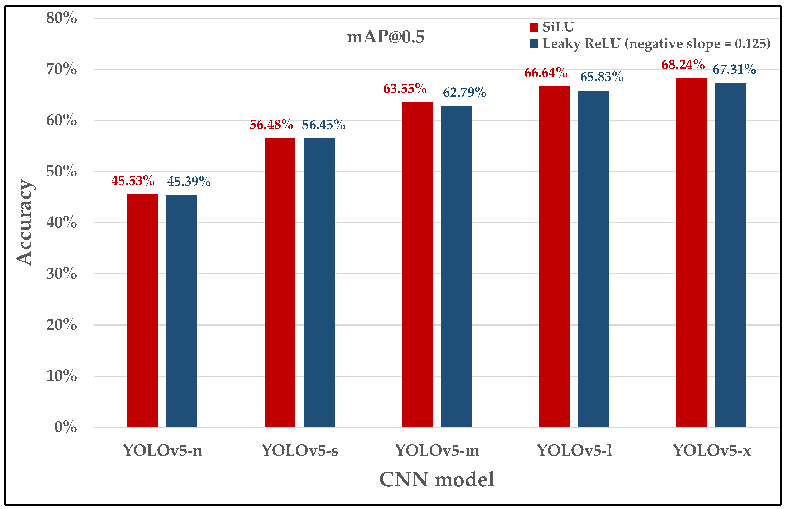
• Simplify the complex activation functions to hardware-friendly functions, which significantly saves computation time and hardware resources.

The remainder of this paper is organized as follows. Section 2 discusses the advantages and disadvantages of various quantization methods, Section 3 presents the details of the proposed quantization method (USPIQ), Section 4 evaluates its performance, and Section 5 includes the conclusions.

2. CNN Quantization

Quantization is the process of reducing the precision of the trained parameters (weights and biases) and activations to reduce the memory and computational requirements of a neural network. It can be categorized into two techniques: training-based quantization and post-training quantization. Training-based quantization is considered an effective method to resolve accuracy degradation issues. However, this requires modifying the training framework and retraining the model, which demands access to the training dataset, a resource that may not be accessible in some applications [16]. In contrast, post-training quantization does not require retraining; thus, the full dataset is unnecessary, which is an important advantage over training-based quantization. However, it often incurs degradation in accuracy after quantization. The two methods are described in detail below.

2.1. Training-Based Quantization

Training-based quantization modifies and retrains the model to recover the accuracy degradation incurred by the process of reducing precision [14,16,17,18,40,41]. In the training-based quantization methods, the backpropagation is conducted on modified paths in their quantization blocks. As a result, they have a problem related to the non-differentiability nature of the quantization blocks. This problem can be alleviated by applying a Straight Through Estimator (STE), which approximates the rounding operation of the gradient to 1 [40,42]. This trains the model using floating-point parameters, and thus the backpropagation manipulates data and stores the outputs in floating-point numbers. Its forward pass uses fixed-point numbers obtained via a quantization operation. For batch normalization, the normalization parameters are folded into weights before the quantization operation. This step is important to match the training results with the final quantized values [32].

2.2. Post-Training Quantization

Post-training quantization starts with the pre-trained full-precision model directly, with no additional retraining, and thus it can provide a faster quantization process with fewer resources than training-based quantization. While it does not require a full dataset, some post-training quantization employs calibration techniques to quantize the output activations. Unfortunately, many previous post-training quantization methods do not provide systematic approaches to mitigating the large quantization errors incurred by low-bit quantization [14]. The advantages and disadvantages of each quantization method are summarized below:

• Accuracy: Training-based quantization often gives higher accuracy than post-training quantization.
• Computational complexity: Post-training quantization can offer a lower computation complexity.
• Model size: Training-based quantization often produces a smaller model size since it retrains the model with reduced precision from the beginning.
• Hyperparameter selection: Post-training quantization requires fewer hyperparameters that need to be tuned.
• Dataset requirement: Post-training quantization does not require a full training dataset, whereas training-based quantization requires a full dataset.

Our proposed hybrid quantization method, USPIQ, combines the best aspects of both methods while avoiding their disadvantages. The proposed method requires training data and backpropagation, so it is categorized as Level 3 quantization among the 4 levels defined by [16]. USPIQ eliminates the need for fine-tuning the hyperparameters during training or after model quantization.

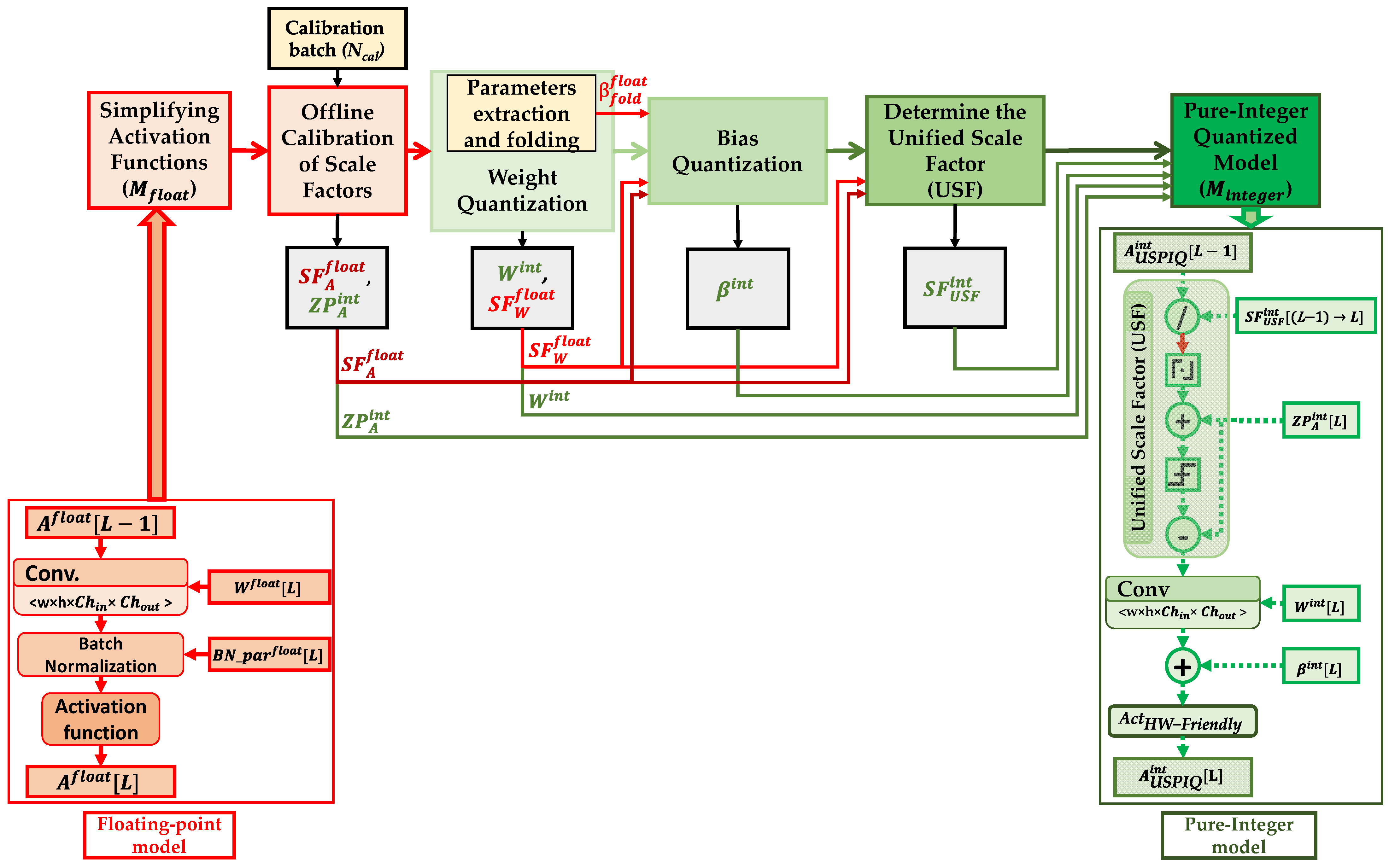
3. Proposed Unified Scaling-Based Pure-Integer Quantization

USPIQ is an efficient quantization method that only requires pure-integer operators in neural network processing units (NPUs) or accelerator hardware while offering higher accuracy than other quantization methods. Figure 1 illustrates the overall flow of the USPIQ method.

USPIQ mainly consists of seven steps, as shown in Algorithm 1. Step 1 simplifies the original CNN model’s complex activation functions to allow pure-integer operations, and then retrains the new CNN model for a short period of epochs to recover any accuracy degradation. Step 2 is the CNN model’s scale factors calibration which is essential for bias quantization and activation outputs scaling; it collects the model statistics ($A_{max}$ and $A_{min}$) using a batch of calibration images $N_{cal}$ and determines the scaling parameters ($S{F}_A^{float}$ and $Z{P}_A^{int}$) of activations in each layer. In this work, we chose the asymmetric mode for quantizing the activation outputs because of its ability to represent the zero value exactly in the integer values, which is vital for layers with zero padding. Step 3 is weight quantization, which employs a variant of asymmetric quantization, where the zero-point values are used to adjust the quantized weights. Step 4 uses an efficient bias quantization method based on the weight and activation scale factors. Step 5 determines the unified integer scale factor $S{F}_{USF}^{int}$, which is used to quantize each layer’s activation outputs. Step 6 independently optimizes the unified scale factor $S{F}_{USF}^{int}$ per connection to effectively balance the skip connections. Finally, step 7 produces a pure-integer CNN model.

Algorithm 1: Unified Scaling-Based Pure-Integer Quantization (USPIQ) method

Inputs: Pre-trained floating-point model Mfloat, a batch of images for calibration Ncal, and user-defined bit precision k. Outputs: Pure-integer CNN model Minteger, quantized (weights $W^{int}$ and biases ${\beta }^{int}$), per-layer unified scale factors $S{F}_{USF}^{int}$, and zero-points $Z{P}_A^{int}$. Algorithm:  1.  Simplify activation functions to hardware-friendly functions.  2.  Calibrate scale factors for activation functions.  3.  Quantize the weights # To determine $W^{int}$ and scale factors $S{F}_A^{float}$.  4.  Quantize the biases # To determine ${\beta }^{int}$, and enable a pure-integer quantization.  5.  Determine the unified scale factor (USF) $S{F}_{USF}^{int}$ for every layer.  6.  Optimize USF for skip connections and align the scale factors.  7.  Return quantized model Minteger and its quantized parameters: $W^{int}$, ${\beta }^{int}$, $S{F}_{USF}^{int}$, and $Z{P}_A^{int}$.

3.1. Simplifying Activation Functions

Step 1 of Algorithm 1 aims to simplify the original CNN model’s complex activation functions that make it impossible to realize them using only pure-integer operations. From extensive experiments with various CNN models, we discovered that activation functions are often highly complex floating-point operations consisting of division, exponential, or logarithmic operations, and consequently, they cannot be converted into pure-integer operations. For example, SSD employs a sigmoid activation function [11,43]; recent models such as YOLOv4 [44] and YOLOv5 [45] use more complex activation functions, MISH and Sigmoid Linear Unit (SiLU), respectively. In Algorithm 1, Step 1 replaces the complex nonlinear activation functions using a simpler partially linear activation function, such as ReLU and Leaky ReLU. For example, YOLOv5 replaces its complex SiLU function using Leaky ReLU with a slope of 1/2ⁿ for negative inputs. Using the slope in the form of 1/2ⁿ instead of an arbitrary slope allows for a hardware-friendly implementation ($Ac{t}_{HW-Friendly}$), such as a shifter instead of a floating-point divider. Figure 2 demonstrates that for all YOLOv5 models, replacing the original activation function and then retraining the model using the COCO 2017 dataset incurs a negligible accuracy degradation of less than 1% compared with the original model.

Furthermore, our extensive experiment assures that the simplified activation function $Ac{t}_{HW-Friendly}$ in the quantized model substantially reduces computation time. For example, the computation time and hardware size of $Ac{t}_{HW-Friendly}$ are reduced by 98.76% and 85%, respectively, compared to SiLU.

3.2. Symmetricity of Value Range

The asymmetric quantization in step 2 of Algorithm 1 allows for the direct representation of zero in the integer values. Equations (1) and (2) determine the scale factor SF and zero-point $ZP$ for the activation outputs or weight parameters, which serve as the foundation for our approach.

$$SF=\frac{x_{max}-x_{min}}{2^k-1}$$

(1)

$$ZP=Clip(\lceil \frac{0-x_{min}}{SF}\rfloor , 0, 2^k-1)$$

(2)

Here, $x_{max}$ and $x_{min}$ indicate the maximum and minimum values, respectively, of the activation outputs or trained weights, which in turn determine the entire range of activations or weights. In Equation (2), $\lceil .\rfloor$ represents rounding the value to the nearest integer number, and the clipping function is defined as in Equation (3).

$$Clip\left(a, b, c\right)=\{\begin{array}{l}b, a<b; Lower limit \\ a, b\le a\le c; Scaled/Quantized value\\ c, a>c; Upper limit \end{array}$$

(3)

3.3. Offline Calibration of Scale Factors

The activation values in a neural network dynamically change depending on the input to the model. Therefore, calculating the scale factors and zero points in Equations (1) and (2) requires calibrating these parameters using a representative batch of unlabeled images; Algorithm 2 outlines the process for offline scale factor calibration. Algorithm 2 takes as input the pre-trained model M_float and a batch of N_cal images for calibration. It then iterates over each layer in M_float, and statistically determines the minimum $A_{min}$ and maximum $A_{max}$ values from the activation outputs of each layer.

Algorithm 2: Offline Calibration of Scale Factors

Inputs: Pre-trained floating-point model Mfloat, a batch of images for calibration Ncal,    the number of layers $N_{Layers}$, and the number of bits k for the quantized values Outputs: Mean scale factor $S{F}_A^{float}\left[L\right]$ and rounded mean zero-point $Z{P}_A^{int}\left[L\right]$ for all layers. Algorithm:  1.  $SumOfS{F}_A^{float}\left[L\right]=0; SumOfZ{P}_A^{int}\left[L\right]=0$ # Initialize the global variables.  2.  for $img$ = 0 to $\left(N_{cal}-1\right)$      # Repeat overall calibration images.  3.  for L = 0 to $\left(N_{Layers}-1\right)$    # Repeat over all layers  4.  $A_{max}\left[img\right]\left[L\right]$ = Find the maximum activation in img in layer $L$ # Collect model statistics.  5.  $A_{min}\left[img\right]\left[L\right]$ = Find the minimum activation in img in layer $L$ # Collect model statistics.  6.  $S{F}_A^{float}\left[img\right]\left[L\right]=\left(\frac{A_{max}\left[img\right]\left[L\right]-A_{min}\left[img\right]\left[L\right]}{2^k-1}\right)$# Activation scale factor of layer (L).  7.  $SumOfS{F}_A^{float}\left[L\right]+=S{F}_A^{float}\left[img\right]\left[L\right]$# Accumulate activation scale factor values.  8.  $Z{P}_A^{int}\left[img\right]\left[L\right]=Clip(\lceil \frac{0-A_{min}\left[img\right]\left[L\right]}{S{F}_A^{float}\left[img\right]\left[L\right]}\rfloor , 0, 2^k-1)$# Zero-point of layer (L).  9.  $SumOfZ{P}_A^{int}\left[L\right]+=Z{P}_A^{int}\left[img\right]\left[L\right]$# Accumulate the zero-point values.  10.  end # end of the model layers.  11.  end # end of the calibration batch.  12.  for $L$ = 0 to $\left(N_{Layers}-1\right)$ # # Repeat over all layers  13.  $S{F}_A^{float}\left[L\right]=\frac{SumOfS{F}_A^{float}\left[L\right]}{N_{cal}}$ #Determine the final mean, $S{F}_A^{float}$, for each layer.  14.  $Z{P}_A^{int}\left[L\right]=\lceil \frac{SumOfZ{P}_A^{int}\left[L\right]}{N_{cal}}\rfloor$ # Determine the final rounded mean, $Z{P}_A^{int}$, for all layers.  15.  end # end of data calibration

To calculate the activations scale factor $S{F}_A^{float}$ and activations zero-point $Z{P}_A^{int}$ for the activation outputs of each layer, Algorithm 2 uses Equations (4) and (5), which are extended from the fundamental Equations (1) and (2). Equations (4) and (5) determine the average scale factor $S{F}_A^{float}\left[L\right]$ and rounded average zero-point $Z{P}_A^{int}\left[L\right]$ values for the activations in each layer L for all N_cal images. These values are used in the next quantization step for bias quantization and the USF calculations described in Section 3.5 and Section 3.6.

$$S{F}_A^{float}\left[L\right]=\frac{1}{N_{cal}}{\displaystyle \sum }_0^{N_{cal}-1 }\frac{\left(A_{max}\left[L\right]-A_{min}\left[L\right]\right)}{2^k-1}$$

(4)

$$Z{P}_A^{int}\left[L\right]=\lceil \frac{1}{N_{cal}}{\displaystyle \sum }_0^{N_{cal}-1}Clip(\lceil \frac{0-A_{min}\left[L\right]}{S{F}_A^{float}\left[L\right]}\rfloor , 0, 2^k-1)\rfloor$$

(5)

3.4. Weight Quantization

In Step 3 of Algorithm 1, the weight quantization process starts by categorizing each parameter to either a weight or a batch normalization parameter and then determines the parameter values in each layer L. The next step is to fold these batch normalization parameters, which entails integrating batch normalization parameters, such as variance, mean, scaling, and shift factor, into the weights and biases of a neural network. This folding process reduces the number of parameters that need to be quantized and stored, and thus it makes the quantization process more efficient.

$$Fma{p}_{conv}^{float}\left[L\right]=Conv\left(W^{float}\left[L\right],A\left[L-1\right]\right)$$

(6)

Equation (6) represents the feature map data obtained by floating-point convolution operation, where $Fma{p}_{conv}^{float}\left[L\right]$, $W^{float}$, and $A^{float}\left[L-1\right]$ represent the floating-point convolution output, weight parameters, and input activations, respectively.

$$A^{float}\left[L\right]=Act\left(\frac{\left(Fma{p}_{conv}^{float}\left[L\right]-E^{float}\left(x_{mini-batch}\right)\left[L\right]\right)\times {\rho }^{float}\left[L\right]}{\sqrt{Va{r}^{float}\left(x_{mini-batch}\right)\left[L\right]+ϵ}}+{\beta }^{float}\left[L\right]\right)$$

(7)

Equation (7) shows the activation output $A^{float}\left[L\right]$ (before parameter folding), where $Va{r}^{float}\left(x_{mini-batch}\right)\left[L\right]$ and $E^{float}\left(x_{mini-batch}\right)\left[L\right]$ represent the variance and mean, respectively, of the mini-batch of images $x_{mini-batch}$ during the training process, whereas $Act()$ represents the activation function. The scaling and bias values for batch normalization, denoted by ${\rho }^{float}\left[L\right]$ and ${\beta }^{float}\left[L\right]$, respectively, are the trainable parameters determined during the training process. Epsilon $ϵ$ is added to the denominator for numerical stability.

Using the definition in Equation (6), we can rewrite Equation (7) as shown in Equation (8).

$$A^{float}\left[L\right]=Act\left(\frac{\left(Conv\left(W^{float}\left[L\right],A^{float}\left[L-1\right]\right)-E^{float}\left(x_{mini-batch}\right)\left[L\right]\right)\times {\rho }^{float}\left[L\right]}{\sqrt{Va{r}^{float}\left(x_{mini-batch}\right)\left[L\right]+ϵ}}+{\beta }^{float}\left[L\right]\right)$$

(8)

The batch normalization parameters in Equations (7) and (8) are pre-determined by the training process but remain constant during the inference. Hence, we can fold these parameters into weights $W_{fold}^{float}\left[L\right]$ and biases ${\beta }_{fold}^{float}\left[L\right]$ using Equations (9) and (10).

$$W_{fold}^{float}\left[L\right]=\frac{W^{float}\left[L\right]\times {\rho }^{float}\left[L\right]}{\sqrt{Va{r}^{float}\left(x_{mini-batch}\right)\left[L\right]+ϵ}}$$

(9)

$${\beta }_{fold}^{float}\left[L\right]= -\frac{E^{float}\left(x_{mini-batch}\right)\left[L\right]\times {\rho }^{float}\left[L\right]}{\sqrt{Va{r}^{float}\left(x_{mini-batch}\right)\left[L\right]+ϵ}}+{\beta }^{float}\left[L\right]$$

(10)

We then use the folded parameters from Equations (9) and (10) in Equation (8) to obtain a compressed expression of Equation (11).

$$A^{float}\left[L\right]=Act\left(Conv\left(W_{fold}^{float}\left[L\right], A^{float}\left[L-1\right]\right)+{\beta }_{fold}^{float}\left[L\right]\right)$$

(11)

Equations (12) and (13) represent scale factor $S{F}_W^{float}\left[L\right]$ and zero point $Z{P}_w^{int}\left[L\right]$ for weight quantization, respectively.

$$S{F}_W^{float}\left[L\right]=\frac{W_{fold}^{float}\left(max\right)\left[L\right]-W_{fold}^{float}\left(min\right)\left[L\right]}{2^k-1}$$

(12)

$$Z{P}_w^{int}\left[L\right]=Clip(\lceil \frac{0-W_{fold}^{float}\left(min\right)\left[L\right]}{S{F}_W^{float}\left[L\right]}\rfloor , 0, 2^k-1)$$

(13)

Equation (14) shows the modified asymmetric mode of weight quantization, where weight zero-point $Z{P}_w^{int}\left[L\right]$ is used to adjust the quantized weight $W^{int}\left[L\right]$ after weight scaling and rounding, which reduces the computation cost as well as the storage.

$$W^{int}\left[L\right]=Clip\left((\lceil \frac{W_{fold}^{float}\left[L\right]}{S{F}_W^{float}\left[L\right]}\rfloor +Z{P}_w^{int}\left[L\right]), 0, 2^k-1\right)-Z{P}_w^{int}\left[L\right]$$

(14)

Algorithm 3 outlines the procedure of quantizing the weights of a neural network; it takes as input the pre-trained model and a user-defined bit precision k while producing outputs, including the integer weights $W^{int}\left[L\right]$, weight scale factors $S{F}_W^{float}\left[L\right]$ and folded biases ${\beta }_{fold}^{float}\left[L\right]$.

Algorithm 3: Weight Quantization

Inputs: Pre-trained floating-point model Mfloat, the number of layers $N_{Layers}$, and bit precision $k$. Outputs: Quantized weights in k-bit integer $W^{int}\left[L\right]$, weight scale factor $S{F}_W^{float}\left[L\right]$, and ${\beta }_{fold}^{float}\left[L\right]$. Algorithm:  1.  Collect and categorize all pre-trained model Mfloat parameters.  2.  for L = 0 to $\left(N_{Layers}-1\right)$                          # Repeat overall $N_{Layers}$ layers  3.  $W_{fold}^{float}\left[L\right]=\frac{W^{float}\left[L\right]\times {\rho }^{float}\left[L\right]}{\sqrt{Va{r}^{float}\left(x_{mini-batch}\right)\left[L\right]+ϵ}}$                 # Fold the batch normalization parameters.  4.  ${\beta }_{fold}^{float}\left[L\right]=-\frac{E^{float}\left(x_{mini-batch}\right)\left[L\right]\times {\rho }^{float}\left[L\right]}{\sqrt{Va{r}^{float}\left(x_{mini-batch}\right)\left[L\right]+ϵ}}+{\beta }^{float}\left[L\right]$# Fold the batch normalization parameters.  5.  $S{F}_W^{float}\left[L\right]=\frac{W_{fold}^{float}\left(max\right)\left[L\right]-W_{fold}^{float}\left(min\right)\left[L\right]}{2^k-1}$         # Calculate weight scale factor.  6.  $Z{P}_w^{int}\left[L\right]=Clip(\lceil \frac{0 - W_{fold}^{float}\left(min\right)\left[L\right]}{S{F}_W^{float}\left[L\right]}\rfloor , 0, 2^k-1)$     # Calculate weight zero-point.  7.  $W^{int}\left[L\right]=Clip\left(\left(\lceil \frac{W_{fold}^{float}\left(min\right)}{S{F}_W^{float}\left[L\right]}\rfloor +Z{P}_w^{int}\left[L\right]\right), 0, 2^k-1\right)-Z{P}_w^{int}\left[L\right]$# Weight Quantization.  8.  end # end of weight quantization

3.5. Bias Quantization

Most previous works have primarily focused on quantizing the weights and activations in convolutional layers while keeping the bias terms in a floating-point format due to the lack of a systematic method to convert all parameters to pure-integer values without incurring accuracy loss. In contrast, our proposed method converts all the parameters, including the bias values, to integer values. As a result, it quantizes the folded floating-point bias terms ${\beta }_{fold}^{float}\left[L\right]$ into integer ${\beta }^{int}\left[L\right]$, which are often small in magnitude, as described in Equation (15), and then adds them directly to the output of the convolutional layers, making the output quantization more accurate without causing a significant accuracy loss.

$${\beta }^{int}\left[L\right]=\lceil \frac{{\beta }_{fold}^{float}\left[L\right]}{S{F}_A^{float}\left[L\right]\times S{F}_W^{float}\left[L\right]}\rfloor$$

(15)

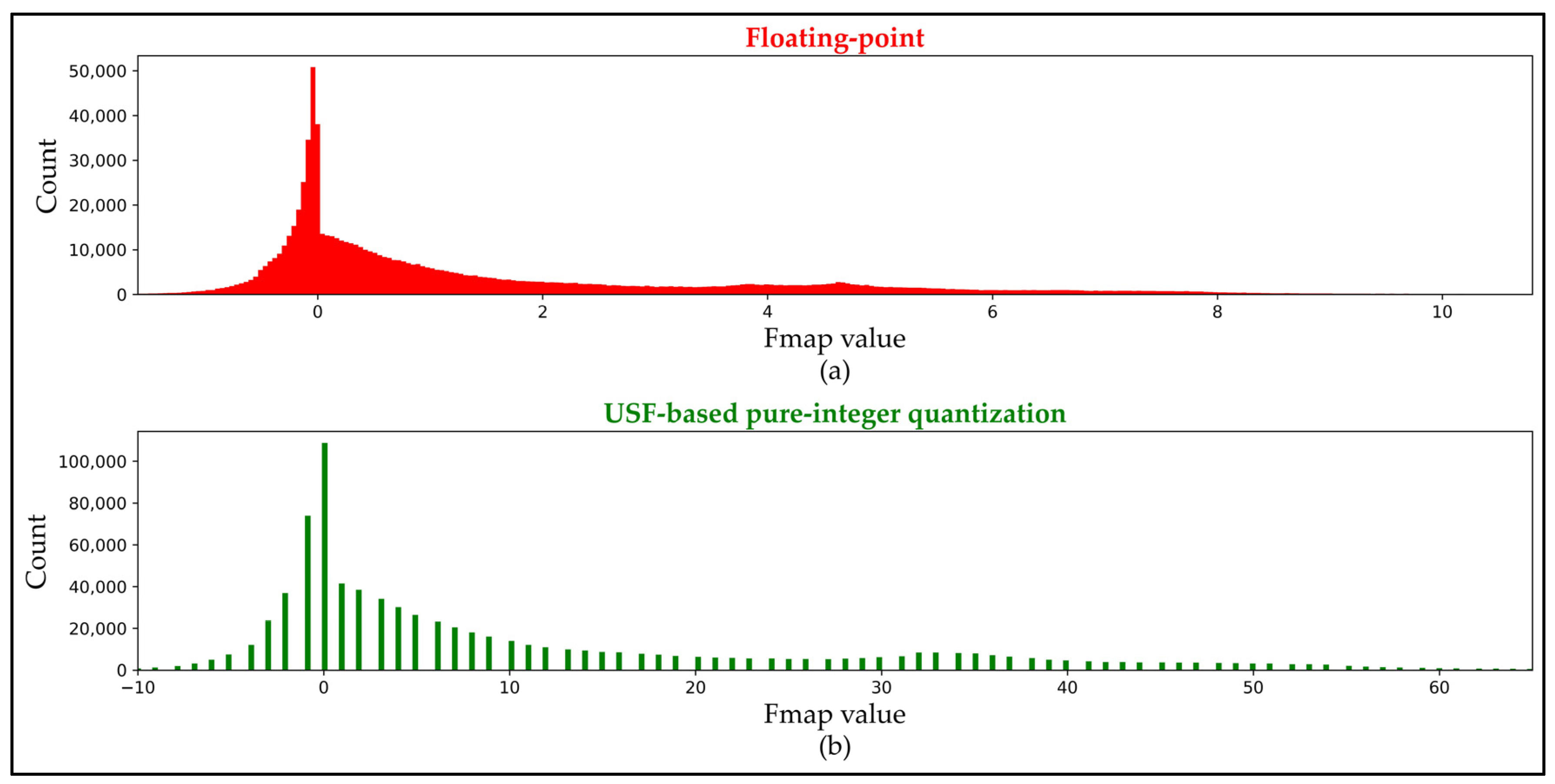
3.6. Proposed Unified Scale Factor (USF)

As discussed above, most previous works have the drawback that only the convolution operations are quantized to integer operations. Due to this restriction, the previous works require an extra conversion operation: (1) quantize the inputs to integer values before the convolutional operation; (2) dequantize the output of convolution operations back to floating-point values for the remaining processes. The extra conversion operations require hardware that supports both integer and floating-point operations, which leads to little or no reduction in hardware resources and chip size. To address these issues, we introduced a notion called unified scale factor (USF) shown in Figure 3, which ensures that all parameters in the quantized model are exclusively integers.

$$S{F}_{USF}^{int}\left[\left(L-1\right)\to L\right]=\lceil \frac{S{F}_A^{float}\left[L\right]}{S{F}_A^{float}\left[L-1\right]\times S{F}_W^{float}\left[L-1\right]}\rfloor$$

(16)

Equation (16) shows the offline calculation of the USF processed by the software for the unified scale factor of the current layer ($L$) with respect to the previous layer $\left(L-1\right)$. This approach ensures that the final unified scale factor of each activation layer’s output $S{F}_{USF}^{int}\left[\left(L-1\right)\to L\right]$ is determined by the activation scale factor of the previous layer $S{F}_A^{float}\left[L-1\right]$, the activation scale factor of the current layer $S{F}_A^{float}\left[L\right]$, and the weight scale factor of the previous layer $S{F}_W^{float}\left[L-1\right]$. Furthermore, by employing the unified scale factor of Equation (16), Equation (17) allows for the online computation of the scaled input activation $A_{USPIQ\left(scaled\right)}^{int}$ using only pure-integer operations.

$$A_{USPIQ\left(scaled\right)}^{int}\left[L-1\right]=Clip\left(\left(\lceil \frac{A_{USPIQ}^{int}\left[L-1\right]}{S{F}_{USF}^{int}\left[\left(L-1\right)\to L\right]}\rfloor +Z{P}_A^{int}\left[L\right]\right), 0, 2^k-1\right)-Z{P}_A^{int}\left[L\right]$$

(17)

Equation (18) gives the pure-integer output activation $A_{USPIQ}^{int}\left[L\right]$ obtained by applying Equations (14)–(17).

$$A_{USPIQ}^{int}\left[L\right]=Ac{t}_{HW-Friendly}\left(Conv\left(W^{int}\left[L\right], A_{USPIQ\left(scaled\right)}^{int}\left[L-1\right]\right)+{\beta }^{int}\left[L\right]\right)$$

(18)

In Equation (18), $A_{USPIQ\left(scaled\right)}^{int}\left[L-1\right]$ represents the scaled input activations in k-bit integers (the integer form replacing the floating-point activations $A^{float}\left[L-1\right]$ in Equation (11)), whereas $W^{int}\left[L\right]$ and ${\beta }^{int}\left[L\right]$ represent the integer weights and biases, respectively. $A_{USPIQ}\left[L\right]$ is the final output activation of layer (L), which in turn represents the input activation for the next layer (L + 1). By applying the hardware-friendly activation function $Ac{t}_{HW-Friendly}$ in Equation (18), we achieved pure-integer computation of all operations, including convolutional operations, bias adding, activation operations, and input activation scaling. In this way, only the final output activations of Equation (18) are stored in the NPU’s on-chip memory, whereas all other intermediate values, such as feature maps (Fmaps) and scaled data, are calculated on-the-fly by the hardware operators.

3.7. Proposed USF-Based Approach for Handling Skip Connections

The demand for training deeper neural networks has increased in recent years due to the increasing demand for more complex AI applications and the advancement of accelerator hardware for CNNs. Residual networks (ResNets) [46] have emerged as an effective solution for training deeper networks by introducing skip connections between layers, which can solve the vanishing or exploding gradient problem. Many complex CNN models commonly employ such skip connections. We demonstrate the proposed method using the YOLOv5-n model as a running example. It comprises more than 60 layers and incorporates 24 skip connections. Figure 4a illustrates the skip connection between the third and sixth layers of YOLOv5-n. However, when quantizing these networks in a naïve way, such challenges arise that the networks require a wider bit-width integer or even floating-point operations to avoid accuracy loss due to the multiple skip connections that are split and then merged by an element-wise adder or concatenation. Conventional methods often employ costly dequantization and quantization steps and use floating-point computations. One such conventional method is the ONNX Run-Time dynamic quantization method [47], as illustrated in Figure 4b.

To address these challenges, our proposed approach introduces a unified scale factor (USF) and independently optimizes the USF per connection; this can effectively eliminate the need for such costly wide-integer or floating-pointer operations. In this way, we can significantly reduce the accuracy degradation while substantially decreasing the cost of computation delay and hardware size. Furthermore, this approach can be generalized for any skip connections that are merged by a merge operation, such as an element-wise adder or concatenation. It is a promising solution for quantizing complex deep neural networks with skip connections, such as ResNets, DenseNet, and YOLOv5.

Figure 4c shows how the two connections (main and skip) of layer ($L-1$) are independently scaled, and their scaled activation outputs are aligned during the merging process. The main connection on the left-hand side is scaled by a separate unified scale factor $S{F}_{USF}^{int}\left[\left(L-1\right)\to L\right]$ between layer ($L-1$) and layer ($L$). The skip connection on the right-hand side is scaled by another independent unified scale factor $S{F}_{USF}^{int}\left[\left(L-1\right)\to \left(L+2\right)\right]$, which aligns the range of the scaled data between the layer ($L-1$) and layer ($L+2$). This skip connection’s scaled input activation represents the first operand (right-hand side) of the element-wise adder, whereas the main connection’s scaled output activation provides the second operand (left-hand side). The two activation data on the two connections are obtained using Equation (16), which determines the optimal activation scale factors for each connection ($S{F}_{USF}^{int}\left[\left(L-1\right)\to \left(L+2\right)\right]$ and $S{F}_{USF}^{int}\left[\left(L+1\right)\to \left(L+2\right)\right]$), followed by Equation (17), which scales the output activation.

Figure 5 compares the element-wise adder results of the original floating-point model (Figure 5a) and the quantized model provided by our proposed approach (Figure 5b) for the example in Figure 4. As shown in Figure 5, the histogram of the output tensor remains nearly unchanged after quantizing the entire layer using the USF-based approach, indicating that the proposed quantization process does not alter the distribution of the output tensor values.

Figure 6a,b illustrates another quantization example for skip connections merged by the concatenation operation. The USF-based approach again uses Equations (16) and (17) with the same numerator ($S{F}_A^{float}\left[L+3\right]$) for layers ($L+2$) and ($L_{right}$) since the next layer after concatenation is ($L+3$).

To describe the key operations of the proposed method, weights, biases, batch normalization parameters, and activation functions were omitted from Figure 6a for simplicity. The quantized model in Figure 6b is obtained by applying the proposed method to Figure 6a. The histograms of the concatenation operation in Figure 6 are shown in Figure 7a for the original model and Figure 7b for the quantized model. As in the above example in Figure 5, the proposed quantized model in Figure 7b shows the distribution of the output data, which is nearly identical to that of the original model.

While the previous two examples illustrate skip connections merged by an element-wise adder and skip connections merged by concatenation, Figure 8 illustrates yet another example that combines the two skip connection types.

The proposed method can determine the appropriate activation scale factors for quantizing the two types of skip connections. Figure 9 demonstrates the effectiveness of the USF-based approach, where the histogram distribution of the output data is nearly unchanged before (Figure 9a) and after (Figure 9b) scaling of the output data into a k-bit integer.

To further demonstrate the versatility of our proposed method for handling various types of skip connections, Figure 10 illustrates the challenging problem of quantizing two distant layers that are merged by concatenation. Figure 10a shows a portion of the original YOLOv5-n (from Layer 14 to Layer 40), where Layer 14, denoted by ($L-1$), has two output connections: one directly connected to its next layer (Layer 15), denoted by ($L$), and the other connected to a concatenation operation (25 layers away) by a skip connection.

Figure 10b illustrates the resulting layers quantized using the USF-based approach from the layers shown in Figure 10a. The USF-based approach scales the two output connections independently: the first connection (right-hand side) from layer ($L-1$) to layer ($L$) is scaled by the unified scale factor $S{F}_{USF}^{int}\left[\left(L-1\right)\to L\right]$, whereas the second connection (left-hand side) from layer ($L-1$) to layer ($L+26$) is scaled by the unified scale factor $S{F}_{USF}^{int}\left[\left(L-1\right)\to \left(L+26\right)\right]$. The above two activation scale factors are determined in a way that provides an optimal range for the activation outputs fed to the next layers, ($L$) and ($L+26$). The concatenation layer has two input connections. The right input connection is the second connection from layer ($L-1$) to layer ($L+26$), which is scaled as described above. On the other hand, the left input connection is scaled using the unified scale factor $S{F}_{USF}^{int}\left[\left(L+25\right)\to \left(L+26\right)\right]$, which optimizes the range of output activations for layer ($L+26$).

Figure 11 compares the output data of the concatenation operation in Figure 10. The histograms of the output data of the original floating-point layer (Figure 11a) and the quantized layer (Figure 11b) are nearly the same.

All the results in Figure 5, Figure 7, Figure 9 and Figure 11 demonstrate the effectiveness and versatility of our proposed method.

4. Performance Evaluation

The proposed quantization method USPIQ has been evaluated using all different versions of YOLOv5 varying in depth from 60 for the nano version (YOLOv5-n) up to 126 parameterized layers for the extra-large version (YOLOv5-x). The USPIQ quantization method is proven superior in all tested versions; the accuracy degradation remained below 0.61% even for the largest YOLOv5 version (YOLOv5-x). The resulting quantized model was evaluated using the COCO val2017. To the best of our knowledge, this is the first study to produce entirely pure-integer quantization for intensive CNN models that consist of complex structures such as skip connections, concatenation, up-sampling, and element-wise addition, without the need for any floating-point calculations. Fundamental PyTorch libraries were employed in all experiments for essential tasks, such as parameter extraction, scale factor calibration, and creating pure-integer inference models. Additionally, the standard Python programming language, complemented by (numpy, pandas, mlflow, tqdm, pillow, seaborn, and scikit-learn libraries) was utilized to quantify weights and biases and calculate per-layer USF values.

Table 1. Detection accuracy ([email protected]) of six YOLOv5 models evaluated on the COCO val2017 dataset for the original models (32-bit floating-point) and their quantized models (8-bit integer).

CNN Model	Number of Parameterized Layers	Floating-Point 32	ONNX Run-Time		USPIQ (Proposed)
			Dynamic	Static
YOLOv5-n (3)	60 (Layer 0 kernel 3 × 3)	43.45%	43.18%	42.91%	43.44%
YOLOv5-n (6)	60 (Layer 0 kernel 6 × 6)	45.39%	43.13%	42.52%	44.80%
YOLOv5-s	60 (Higher channels depth)	56.45%	55.70%	55.09%	55.90%
YOLOv5-m	82	62.58%	62.00%	61.82%	62.18%
YOLOv5-l	104	65.83%	63.39%	65.23%	65.34%
YOLOv5-x	126	67.31%	66.09%	66.29%	66.70%

shows the 8-bit quantization results of various YOLOv5 models with an input image size of 640 × 640.

Table 1 shows that the proposed method (USPIQ) outperforms the ONNX Run-Time quantization methods for all YOLOv5 versions. Furthermore, as shown in Figure 12a, the ONNX Run-Time dynamic still requires floating-point computation in most of the layer’s operations, except for the convolution operation. Therefore, it requires extra hardware to convert the convolution results back to a floating-point format and compute all the remaining operations using floating-point hardware units. In addition, ONNX Run-Time static requires floating-point computation in all of the layer’s operations, as shown in Figure 12b. Hence, the quantized weights and activations offer no reduction in the floating-point operator hardware, but it can reduce the memory size. As a result, both methods of ONNX Run-Time cannot be used for low-power NPUs or accelerator chips composed only of integer operator resources.

Another serious problem in ONNX Run-Time dynamic quantization is that it requires quantization and dequantization processes at every layer on-the-fly during inference execution, which imposes a great burden on accelerator hardware. In contrast, the proposed method completes all quantization processes offline and eliminates the need for any floating-point operations in the entire inference process, as shown in Figure 12c.

Next, we present two experiments to compare the inference computation times of quantized models from the ONNX Run-Time dynamic and the proposed method. The first experiment is based on actual inference on a GPU-based PC, while the second experiment is based on the estimation of computation time on an NPU architecture [48,49]. In the first experiment, the quantized YOLOv5 models are tested using a GPU-based PC with an Intel(R) Core (TM) i7-9700 CPU @ 3.00GHz, GPU NVIDIA GeForce RTX 2060 (6GB).

The proposed USPIQ method achieves a remarkable decrease in inference time compared to ONNX Run-Time dynamic quantization for all YOLOv5 models (USPIQ achieves a speedup of 1.64 to 2.84 times), as shown in

Table 2. The inference time measured on a GPU-based PC for YOLOv5 models (milliseconds) per image of ONNX Run-Time dynamic quantization and the proposed USPIQ.

CNN Model	ONNX Run-Time (Dynamic)	USPIQ (Proposed)
YOLOv5-n (3)	42.00	25.56
YOLOv5-n (6)	48.36	29.28
YOLOv5-s	85.32	41.53
YOLOv5-m	134.41	63.25
YOLOv5-l	282.49	100.20
YOLOv5-x	458.72	162.07

. Table 2 demonstrates that the proposed method offers a substantially higher speed improvement for deeper and more complex CNNs.

In the second experiment, we estimated the computational time based on the NPU architecture simulator reported in [48,49] using YOLOv5-n (3) model, as shown in

Table 3. Estimated computation time (milliseconds) per image based on an NPU architecture simulator for the quantized model of YOLOv5-n (3).

Process	Operation	ONNX Run-Time (Dynamic)	USPIQ (Proposed)
Convolutional	MAC	4.56	4.56
Bias adding		1.09	0.55
Activation function	Shifting	-/-	Negligible
	Division	2.18	-/-
Floating-point quantization		5.46	-/-
Integer unified scaling of activations		-/-	1.91
Element-wise adder		0.023	0.006
Concatenation		0.014	0.004
Max-pooing		0.006	0.002
Up-sampling (Resize)		0.0013	0.0003
Total computational time per image		13.33	7.03

.

Table 3 compares the NPU’s estimated inference time for ONNX Run-Time dynamic and USPIQ. For this estimation, we used an NPU architecture with a clock frequency of 400 MHz, a convolutional processing array consisting of 1152 processing elements (PEs) that conduct 1152 multiply and accumulate (MAC) operations in parallel, and 32 parallel units for post-convolutional operations, including bias adding, unified scaling, up-sampling, max-pooling, and element-wise addition. For ONNX Run-Time dynamic, we added floating-point operators to the NPU simulator, whereas for USPIQ, we only used pure-integer operators in the NPU simulator. Table 3 shows that USPIQ with pure-integer NPU architecture offers an inference time of 7.03 msec per image, which is 47.31% shorter than the 13.33 msec provided by ONNX Run-Time dynamic with partially floating-point NPU architecture.

In addition to reducing the computational cost and memory overhead of storing parameters and activations, USPIQ’s pure-integer inference model can significantly decrease the energy consumption for matrix manipulations in NPUs or accelerator chips. To evaluate the energy savings of USPIQ over ONNX Run-Time, we estimated the energy consumption of the quantized model of YOLOv5-n (3), as shown in

Table 4. Estimated energy consumption (pico Joule) per image based on the NPU architecture simulator and the CMOS 45 nm process energy table for the quantized model of YOLOv5-n (3).

Process	Operation	ONNX Run-Time		USPIQ (Proposed)
		Dynamic	Static
Convolutional	Multiplication	1681.08	7775.01	1681.08
	Addition	210.14	1891.22	210.14
Bias adding		12.57	12.57	1.19
Activation function	Shifting	-/-	-/-	Negligible
	Division	44.00	44.00	-/-
Floating-point quantization		256.06	193.61	-/-
Integer unified scaling of activations		-/-	-/-	21.65
Element-wise adder		1.06	1.06	0.06
Concatenation		0.29	0.29	0.14
Max-pooing		0.28	0.28	0.02
Up-sampling (Resize)		0.06	0.06	0.03
Total energy consumption		2205.54	9918.10	1914.31

.

Energy consumption was estimated by the NPU simulator [48,49] using physical design kit data for a 45 nm CMOS process [12], which provides accurate energy estimation of individual operators in the NPU. For the convolution operations, USPIQ achieves an energy savings of 80.43% over the ONNX Run-Time Static since USPIQ uses only pure-integer operations for convolution, whereas ONNX Run-Time static requires 32-bit floating-point calculations. Furthermore, while both ONNX Run-Time quantization methods use floating-point calculations for bias addition, USPIQ needs only 18-bit integer adder units for bias addition, leading to a significant reduction in energy consumption by ~90%.

In addition, replacing the power-hungry floating-point division of the Leaky ReLU activation function with a simple shift operation made the power consumption of USPIQ’s activation functions negligible compared with ONNX Run-Time quantization. Moreover, our proposed USF eliminates the repetitive power-hungry floating-point scaling of activations in the NPU, reducing the scaling energy consumption by 91.54% and 88.82% compared to the ONNX dynamic and static quantization methods, respectively. In the overall energy consumption of the YOLOv5-n (3) model, the USPIQ with the pure-integer NPU simulator reduces the energy consumption by 13.2% and 80.7%, compared to ONNX Run-Time dynamic and static quantization, respectively.

We also compared our work to other previous work [14], where training-based and post-training quantization for 8-bit were both evaluated using COCO 2017 dataset and EfficientDet-D1 model (with 6.6 million parameters), which is comparable to the YOLOv5-s model in size (7.22 million parameters); in the experiments of [14], their method suffers from an accuracy loss of 1.14% and 1.79%, respectively. In contrast, our work achieves an accuracy loss of only 0.55% compared to the original float-point model.

Table 5. YOLOv5 quantization results with 8-bit and 4-bit integers for the proposed USPIQ and other previous works.

CNN Model	Floating-Point 32	[50] 8-bit	[51] 8-bit	[52] 4-bit	USPIQ (Proposed)
YOLOv5-s6_960_relu (AP50)	86.7%	81.1%	-/-	-/-	85.90% (8-bit)
YOLOv5-m ([email protected])	62.58%	-/-	61.7%	-/-	62.18% (8-bit)
YOLOv5-s ([email protected])	56.45%	-/-	-/-	33.4%	33.90% (4-bit)

shows that YOLO-pose [50], with an input image size of 960x960, reported an unacceptably large accuracy loss of 5.6% for the YOLOv5-s model when quantized using all the 8-bit integers. To reduce the accuracy loss to 1.3%, the quantization was increased to 16-bit integers for 30% of all the layers in YOLOv5-s. However, our proposed method achieves an accuracy loss of only 0.8% using 8-bit pure-integer quantization. In [51], a hardware-friendly log scale quantization method was proposed for YOLOv5-m, which resulted in an accuracy degradation of 0.88% while still utilizing floating-point operations during the inference computation. In contrast, our proposed USPIQ method achieves a significantly smaller accuracy loss of only 0.4%, even with pure-integer operations during the inference.

The work in [52] proposes a hardware-friendly low-precision full quantization method called DRGS and evaluates it for YOLOv5-s using 4-bit integer precision, achieving a [email protected] score of 33.4%. Their approach requires retraining the model to dynamically select rounding modes for weights and scale the corresponding gradient properly, which incurs significant complexity, as well as modifying the training framework. In contrast, our proposed USPIQ method obtains a higher [email protected] score of 33.9% and does not require a complex retraining process or any modifications to the training framework.

5. Conclusions

This study proposes a hybrid quantization method that combines the best aspects of the training-based and post-training methods. The proposed method, Unified Scaling-Based Pure-Integer Quantization (USPIQ), is designed to optimize deep neural networks with complex skip connections for deployment on pure-integer accelerator chips for edge AI devices. USPIQ simplifies integer quantization by systematically converting all internal floating-point operations to pure-integer operations without fine-tuning, unlike the previous methods. Furthermore, USPIQ introduces a new scaling approach called the unified scale factor (USF), which combines quantization and dequantization processes for each layer and connection. By employing USF, USPIQ can entirely eliminate floating-point hardware and significantly reduce the on-chip memory for parameters and activation data in the accelerator chip. USPIQ with pure-integer calculation can also considerably reduce the computational overhead and energy consumption with little accuracy loss, making it well suited to low-power pure-integer NPUs and deep-learning accelerator chips. Our extensive experimental results demonstrate that USPIQ outperforms previous state-of-the-art quantization methods in all aspects of inference speed, accelerator chip size, energy consumption, and inference accuracy. Therefore, USPIQ is a promising method for optimizing complex deep neural networks and deploying them on resource-limited accelerator chips in edge AI devices.

References

1. Krizhevsky, A.; Sutskever, I.; Hinton, G.E. Imagenet classification with deep convolutional neural networks. Commun. ACM 2017, 60, 84–90. [Google Scholar] [CrossRef] [Green Version]
2. Simonyan, K.; Zisserman, A. Very deep convolutional networks for large-scale image recognition. arXiv 2014, arXiv:1409.1556. [Google Scholar]
3. Lybrand, E.; Saab, R. A greedy algorithm for quantizing neural networks. J. Mach. Learn. Res. 2021, 22, 7007–7044. [Google Scholar]
4. Li, R.; Wang, Y.; Liang, F.; Qin, H.; Yan, J.; Fan, R. Fully quantized network for object detection. In Proceedings of the IEEE Conference on Computer Vision and Pattern Recognition (CVPR 2019), Long Beach, CA, USA, 16–20 June 2019; pp. 2805–2814. [Google Scholar]
5. Andriyanov, N.A.; Dementiev, V.E.; Tashlinskii, A.G. Detection of objects in the images: From likelihood relationships towards scalable and efficient neural networks. Comput. Opt. 2022, 46, 139–159. [Google Scholar] [CrossRef]
6. Minderer, M.; Gritsenko, A.; Stone, A.; Neumann, M.; Weissenborn, D.; Dosovitskiy, A.; Mahendran, A.; Arnab, A.; Dehghani, M.; Shen, Z.; et al. Simple open-vocabulary object detection with vision transformers. arXiv 2022, arXiv:2205.06230. [Google Scholar]
7. Zhang, W.; Huang, D.; Zhou, M.; Lin, J.; Wang, X. Open-Set Signal Recognition Based on Transformer and Wasserstein Distance. Appl. Sci. 2023, 13, 2151. [Google Scholar] [CrossRef]
8. Girshick, R.; Donahue, J.; Darrell, T.; Malik, J. Rich feature hierarchies for accurate object detection and semantic segmentation. In Proceedings of the IEEE Conference on Computer Vision and Pattern Recognition (CVPR 2014), Columbus, OH, USA, 24–27 June 2014; pp. 580–587. [Google Scholar]
9. Ren, S.; He, K.; Girshick, R.; Sun, J. Faster r-cnn: Towards real-time object detection with region proposal networks. In Proceedings of the Advances in Neural Information Processing Systems 28 (NeurIPS 2015), Montreal, QC, Canada, 7–12 December 2015; pp. 2969239–2969250. [Google Scholar]
10. Joseph, R.; Farhadi, A. YOLO9000: Better, faster, stronger. In Proceedings of the IEEE Conference on Computer Vision and Pattern Recognition (CVPR 2017), Honolulu, HI, USA, 21–26 July 2017; pp. 7263–7271. [Google Scholar]
11. Liu, W.; Anguelov, D.; Erhan, D.; Szegedy, C.; Reed, S.; Fu, C.Y.; Berg, A.C. Ssd: Single shot multibox detector. In Proceedings of the Computer Vision–ECCV: 14th European Conference, Amsterdam, The Netherlands, 11–14 October 2016; Part I 14. pp. 21–37. [Google Scholar]
12. Han, S.; Pool, J.; Tran, J.; Dally, W. Learning both weights and connections for efficient neural network. In Proceedings of the Advances in Neural Information Processing Systems 28 (NeurIPS 2015), Montreal, QC, Canada, 7–12 December 2015; pp. 1–8. [Google Scholar]
13. Nguyen, D.T.; Nguyen, T.N.; Kim, H.; Lee, H.J. A high-throughput and power-efficient FPGA implementation of YOLO CNN for object detection. IEEE Trans. Very Large Scale Integr. (VLSI) Syst. 2019, 17, 1861–1873. [Google Scholar] [CrossRef]
14. Nagel, M.; Fournarakis, M.; Amjad, R.A.; Bondarenko, Y.; Van Baalen, M.; Blankevoort, T. A white paper on neural network quantization. arXiv 2021, arXiv:2106.08295. [Google Scholar]
15. Chen, S.; Wang, W.; Pan, S.J. Metaquant: Learning to quantize by learning to penetrate non-differentiable quantization. In Proceedings of the Advances in Neural Information Processing Systems 32 (NeurIPS 2019), Vancouver, BC, Canada, 8–14 December 2019; pp. 3918–3928. [Google Scholar]
16. Nagel, M.; Baalen, M.V.; Blankevoort, T.; Welling, M. Data-free quantization through weight equalization and bias correction. In Proceedings of the IEEE/CVF International Conference on Computer Vision (ICCV 2019), Seoul, Republic of Korea, 27 October–2 November 2019; pp. 1325–1334. [Google Scholar]
17. Wang, Z.; Wu, Z.; Lu, J.; Zhou, J. Bidet: An efficient binarized object detector. In Proceedings of the IEEE/CVF Conference on Computer Vision and Pattern Recognition (CVPR 2020), Virtual Conference, 14–19 June 2020; pp. 2049–2058. [Google Scholar]
18. Zhao, S.; Yue, T.; Hu, X. Distribution-aware adaptive multi-bit quantization. In Proceedings of the IEEE/CVF Conference on Computer Vision and Pattern Recognition (CVPR 2020), Virtual Conference, 14–19 June 2020; pp. 9281–9290. [Google Scholar]
19. Gysel, P.; Pimentel, J.; Motamedi, M.; Ghiasi, S. Ristretto: A framework for empirical study of resource-efficient inference in convolutional neural networks. IEEE Trans. Neural Netw. Learn. Syst. 2018, 29, 5784–5789. [Google Scholar] [CrossRef] [PubMed]
20. Banner, R.; Nahshan, Y.; Soudry, D. Post training 4-bit quantization of convolutional networks for rapid-deployment. In Proceedings of the Advances in Neural Information Processing Systems 32 (NeurIPS 2019), Vancouver, BC, Canada, 8–14 December 2019; pp. 7948–7956. [Google Scholar]
21. Cheng, Y.; Wang, D.; Zhou, P.; Zhang, T. A survey of model compression and acceleration for deep neural networks. arXiv 2017, arXiv:1710.09282. [Google Scholar]
22. Wu, H.; Judd, P.; Zhang, X.; Isaev, M.; Micikevicius, P. Integer quantization for deep learning inference: Principles and empirical evaluation. arXiv 2020, arXiv:2004.09602. [Google Scholar]
23. Nogami, W.; Ikegami, T.; Takano, R.; Kudoh, T. Optimizing weight value quantization for cnn inference. In Proceedings of the International Joint Conference on Neural Networks (IJCNN/IEEE), Budapest, Hungary, 14–19 July 2019; pp. 1–8. [Google Scholar]
24. Zhang, J.; Zhou, Y.; Saab, R. Post-training quantization for neural networks with provable guarantees. arXiv 2022, arXiv:2201.11113. [Google Scholar] [CrossRef]
25. Courbariaux, M.; Hubara, I.; Soudry, D.; El-Yaniv, R.; Bengio, Y. Binarized neural networks: Training deep neural networks with weights and activations constrained to+ 1 or-1. arXiv 2016, arXiv:1602.02830. [Google Scholar]
26. Choukroun, Y.; Kravchik, E.; Yang, F.; Kisilev, P. Low-bit quantization of neural networks for efficient inference. In Proceedings of the IEEE/CVF International Conference on Computer Vision Workshop (ICCVW), Seoul, Republic of Korea, 27 October–2 November 2019; pp. 3009–3018. [Google Scholar]
27. Wang, K.; Liu, Z.; Lin, Y.; Lin, J.; Han, S. Haq: Hardware-aware automated quantization with mixed precision. In Proceedings of the IEEE/CVF Conference on Computer Vision and Pattern Recognition (CVPR 2019), Long Beach, CA, USA, 16–20 June 2019; pp. 8612–8620. [Google Scholar]
28. Zhang, X.; Qin, H.; Ding, Y.; Gong, R.; Yan, Q.; Tao, R.; Li, Y.; Yu, F.; Liu, X. Diversifying sample generation for accurate data-free quantization. In Proceedings of the IEEE/CVF Conference on Computer Vision and Pattern Recognition (CVPR 2021), Virtual Conference, 19–25 June 2021; pp. 15658–15667. [Google Scholar]
29. Nagel, M.; Amjad, R.A.; Van Baalen, M.; Louizos, C.; Blankevoort, T. Up or down? adaptive rounding for post-training quantization. In Proceedings of the International Conference on Machine Learning (PMLR 2020), Vienna, Austria, 12–18 July 2020; pp. 7197–7206. [Google Scholar]
30. Liu, Y.; Zhang, W.; Wang, J. Zero-shot adversarial quantization. In Proceedings of the IEEE/CVF Conference on Computer Vision and Pattern Recognition (CVPR 2021), Virtual Conference, 19–25 June 2021; pp. 1512–1521. [Google Scholar]
31. Chikin, V.; Antiukh, M. Data-Free Network Compression via Parametric Non-uniform Mixed Precision Quantization. In Proceedings of the IEEE/CVF Conference on Computer Vision and Pattern Recognition (CVPR 2022), New Orleans, LA, USA, 19–24 June 2022; pp. 450–459. [Google Scholar]
32. Jacob, B.; Kligys, S.; Chen, B.; Zhu, M.; Tang, M.; Howard, A.; Adam, H.; Kalenichenko, D. Quantization and training of neural networks for efficient integer-arithmetic-only inference. In Proceedings of the IEEE/CVF Conference on Computer Vision and Pattern Recognition (CVPR 2018), Salt Lake City, UT, USA, 19–21 June 2018; pp. 2704–2713. [Google Scholar]
33. Al-Hamid, A.A.; Kim, T.; Park, T.; Kim, H. Optimization of Object Detection CNN with Weight Quantization and Scale Factor Consolidation. In Proceedings of the International Conference on Consumer Electronics-Asia (ICCE-Asia/IEEE), Yeosu, Republic of Korea, 26–28 October 2021; pp. 1–5. [Google Scholar]
34. Yamamoto, K. Learnable companding quantization for accurate low-bit neural networks. In Proceedings of the IEEE/CVF Conference on Computer Vision and Pattern Recognition (CVPR 2021), Virtual Conference, 19–25 June 2021; pp. 5029–5038. [Google Scholar]
35. Intel. Intel Distribution of OpenVINO Toolkit. Available online: https://docs.openvinotoolkit.org (accessed on 6 June 2023).
36. Andriyanov, N.; Papakostas, G. Optimization and Benchmarking of Convolutional Networks with Quantization and OpenVINO in Baggage Image Recognition. In Proceedings of the VIII International Conference on Information Technology and Nanotechnology (ITNT/IEEE), Samara, Russia, 23–27 May 2022; pp. 1–4. [Google Scholar]
37. Demidovskij, A.; Tugaryov, A.; Fatekhov, M.; Aidova, E.; Stepyreva, E.; Shevtsov, M.; Gorbachev, Y. Accelerating object detection models inference within deep learning workbench. In Proceedings of the International Conference on Engineering and Emerging Technologies (ICEET/IEEE), Istanbul, Turkey, 27–28 October 2021; pp. 1–6. [Google Scholar]
38. Feng, H.; Mu, G.; Zhong, S.; Zhang, P.; Yuan, T. Benchmark analysis of yolo performance on edge intelligence devices. Cryptography 2022, 6, 16. [Google Scholar] [CrossRef]
39. Kryzhanovskiy, V.; Balitskiy, G.; Kozyrskiy, N.; Zuruev, A. Qpp: Real-time quantization parameter prediction for deep neural networks. In Proceedings of the IEEE/CVF Conference on Computer Vision and Pattern Recognition (CVPR 2021), Virtual Conference, 19–25 June 2021; pp. 10684–10692. [Google Scholar]
40. Zhou, S.; Wu, Y.; Ni, Z.; Zhou, X.; Wen, H.; Zou, Y. Dorefanet: Training low bitwidth convolutional neural networks withlow bitwidth gradients. arXiv 2016, arXiv:1606.06160. [Google Scholar]
41. Park, E.; Ahn, J.; Yoo, S. Weighted-Entropy-Based Quantization for Deep Neural Networks. In Proceedings of the IEEE Conference on Computer Vision and Pattern Recognition (CVPR 2017), Honolulu, HI, USA, 21–26 July 2017; pp. 5456–5464. [Google Scholar]
42. Yang, Y.; Deng, L.; Wu, S.; Yan, T.; Xie, Y.; Li, G. Training high-performance and large-scale deep neural networks with full 8-bit integers. Neural Netw. 2020, 125, 70–82. [Google Scholar] [CrossRef] [PubMed] [Green Version]
43. Elfwing, S.; Uchibe, E.; Doya, K. Sigmoid-weighted linear units for neural network function approximation in reinforcement learning. Neural Netw. 2018, 107, 3–11. [Google Scholar] [CrossRef] [PubMed]
44. Bochkovskiy, A.; Wang, C.Y.; Liao, H.Y.M. Yolov4: Optimal speed and accuracy of object detection. arXiv 2020, arXiv:2004.10934. [Google Scholar]
45. Glenn, J.; Stoken, A.; Chaurasia, A.; Borovec, J.; Kwon, Y.; Michael, K.; Liu, C.; Fang, J.; Abhiram, V.; Skalski, S.P. ultralytics/yolov5: v6.0—YOLOv5n ‘Nano’models, Roboflow Integration, TensorFlow Export, OpenCV DNN Support; Zenodo Tech. Rep. 2021. Available online: https://zenodo.org/record/5563715 (accessed on 12 May 2023).
46. He, K.; Zhang, X.; Ren, S.; Sun, J. Deep Residual Learning for Image Recognition. In Proceedings of the IEEE Conference on Computer Vision and Pattern Recognition (CVPR 2016), Las Vegas, NV, USA, 27–30 June 2016; pp. 770–778. [Google Scholar]
47. ONNX: Open Neural Network Exchange. Available online: https://github.com/onnx/onnx/ (accessed on 13 April 2023).
48. Son, H.; Na, Y.; Kim, T.; Al-Hamid, A.A.; Kim, H. CNN Accelerator with Minimal On-Chip Memory Based on Hierarchical Array. In Proceedings of the 18th International SoC Design Conference (ISOCC/IEEE), Jeju, Republic of Korea, 6–9 October 2021; pp. 411–412. [Google Scholar]
49. Son, H.; Al-Hamid, A.A.; Na, Y.; Lee, D.; Kim, H. CNN Accelerator Based on Diagonal Cyclic Array Aimed at Minimizing Memory Accesses. Comput. Mater. Contin. 2023; accepted. [Google Scholar]
50. Maji, D.; Nagori, S.; Mathew, M.; Poddar, D. YOLO-Pose: Enhancing YOLO for Multi Person Pose Estimation Using Object Keypoint Similarity Loss. In Proceedings of the IEEE/CVF Conference on Computer Vision and Pattern Recognition (CVPR 2022), New Orleans, LA, USA, 19–24 June 2022; pp. 2637–2646. [Google Scholar]
51. Choi, D.; Kim, H. Hardware-friendly log-scale quantization for CNNs with activation functions containing negative values. In Proceedings of the 18th International SoC Design Conference (ISOCC/IEEE), Jeju, Republic of Korea, 6–9 October 2021; pp. 415–416. [Google Scholar]
52. Wu, Q.; Li, Y.; Chen, S.; Kang, Y. DRGS: Low-Precision Full Quantization of Deep Neural Network with Dynamic Rounding and Gradient Scaling for Object Detection. In Proceedings of the Data Mining and Big Data: 7th International Conference, (DMBD), Beijing, China, 21–24 November 2022; pp. 137–151. [Google Scholar]
Figure 1. The flow diagram of the Unified Scaling-Based Pure-Integer Quantization method.
Electronics 12 02660 g001
Figure 2. Retraining different versions of YOLOv5 with hardware-friendly activation functions (replacing SiLU using Leaky ReLU).
Electronics 12 02660 g002
Figure 3. Example of quantization result obtained by applying the proposed method to the first convolutional layer of the YOLOv5-n CNN model: (a) Accelerator hardware structure; (b) quantization process in the software side (USF-USPIQ).
Electronics 12 02660 g003
Figure 4. Comparison of quantization methods for skip connections merged by element-wise adder: (a) The original floating-point model; (b) the partial-integer quantization obtained by ONNX Run-Time dynamic; (c) the proposed USF-based pure-integer quantization method.
Electronics 12 02660 g004
Figure 5. Histogram of element-wise adder output tensors for (a) the floating-point model in Figure 4a; and (b) the quantized model in Figure 4c.
Electronics 12 02660 g005
Figure 6. The quantization method for skip connections merged by concatenation: (a) The original floating-point model; (b) the USF-based pure-integer quantized model.
Electronics 12 02660 g006
Figure 7. Histogram of concatenation output tensors for (a) the floating-point model in Figure 6a; and (b) the quantized model in Figure 6b.
Electronics 12 02660 g007
Figure 8. The quantization method for skip connections merged by an element-wise adder and concatenation: (a) The original floating-point model; (b) the USF-based pure-integer quantized model.
Electronics 12 02660 g008
Figure 9. Histogram of concatenation output tensors for (a) the floating-point model in Figure 8a; and (b) the quantized model in Figure 8b.
Electronics 12 02660 g009
Figure 10. The quantization method for skip connections merged by up-sampling (Resize) and concatenation: (a) The original floating-point model; (b) the USF-based pure-integer quantized model.
Electronics 12 02660 g010
Figure 11. Histogram of the concatenation output tensors for (a) the floating-point model in Figure 10a; and (b) the quantized model in Figure 10b.
Electronics 12 02660 g011
Figure 12. Comparison of quantized model for the first convolutional layer in YOLOv5-n (3): (a) ONNX Run-time dynamic; (b) ONNX Run-Time static; (c) the proposed method USPIQ.
Electronics 12 02660 g012