

Camouflaged Object Detection with a Feature Lateral Connection Network


1
HDU-ITMO Joint Institute, Hangzhou Dianzi University, Hangzhou 310018, China
2
College of Computer Science and Technology, Zhejiang University of Technology, Hangzhou 310014, China
*
Author to whom correspondence should be addressed.
Electronics 2023, 12(12), 2570; https://doi.org/10.3390/electronics12122570
Submission received: 26 April 2023
/
Revised: 23 May 2023
/
Accepted: 2 June 2023
/
Published: 7 June 2023
(This article belongs to the Special Issue Deep and Machine Learning for Image Processing: Medical and Non-medical Applications)
Abstract
:We propose a new framework for camouflaged object detection (COD) named FLCNet, which comprises three modules: an underlying feature mining module (UFM), a texture-enhanced module (TEM), and a neighborhood feature fusion module (NFFM). Existing models overlook the analysis of underlying features, which results in extracted low-level feature texture information that is not prominent enough and contains more interference due to the slight difference between the foreground and background of the camouflaged object. To address this issue, we created a UFM using convolution with various expansion rates, max-pooling, and avg-pooling to deeply mine the textural information of underlying features and eliminate interference. Motivated by the traits passed down through biological evolution, we created an NFFM, which primarily consists of element multiplication and concatenation followed by an addition operation. To obtain precise prediction maps, our model employs the top-down strategy to gradually combine high-level and low-level information. Using four benchmark COD datasets, our proposed framework outperforms 21 deep-learning-based models in terms of seven frequently used indices, demonstrating the effectiveness of our methodology.
1. Introduction
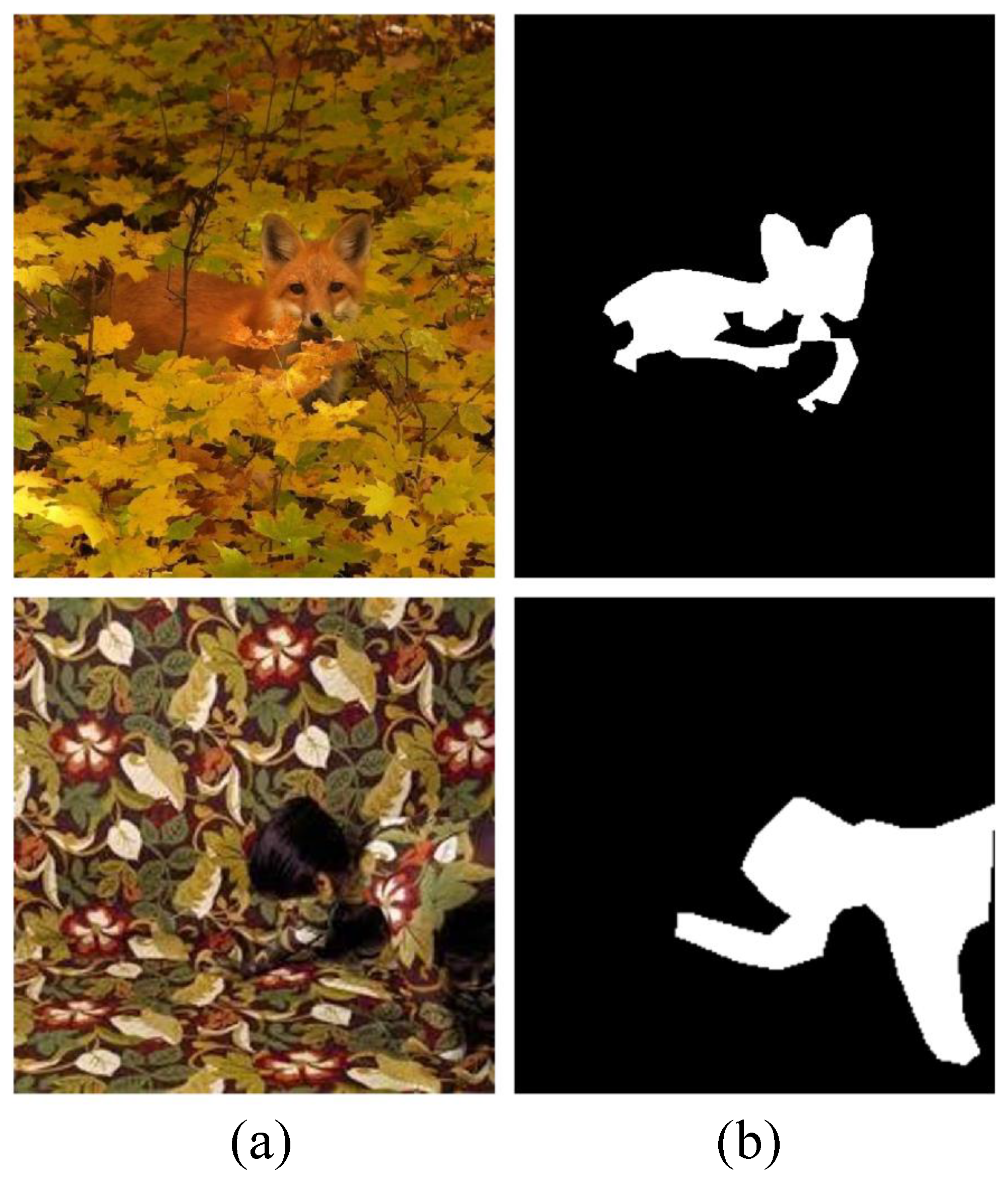
Camouflage is a common biological phenomenon observed in nature that allows organisms to blend into their surroundings, thus avoiding predators [1,2,3]. As shown in Figure 1, we present a camouflaged object and the ground truth (GT). Camouflaged objects include naturally camouflaged and artificially camouflaged objects. Natural camouflage primarily refers to animals that blend in with their surroundings, while artificial camouflage is increasingly used in various fields (such as art, combat, etc.). In contrast to salient object detection (SOD) [4], camouflaged object detection (COD) is more challenging due to the high similarity between the object and the background in terms of texture, color, and shape, resulting in low visual recognition of its boundary and surrounding environment. In addition to its scientific value, studying COD has significant engineering applications (such as surface defect detection, search, rescue, etc.) [5,6].
Research on camouflage can be traced back to 1998. Researchers have proposed various camouflaged object detection methods based on direct visual features (such as color, texture, optical flow, etc.) [7,8]. However, traditional models fail to detect in cases where there is shallow contrast between the foreground and background [9,10]. To overcome this limitation, researchers have recently introduced deep learning into COD and proposed various deep-learning-based models (such as SINet_V2 [11], UGTR [12], C2FNet [13], MGL-R [14], etc.). These models have strong feature extraction abilities and self-learning capacities, which improve the accuracy of camouflaged object detection and boost the model’s generalization.
Similarly, we propose a new deep-learning-based model for camouflaged object detection named feature lateral connection networks (FLCNet), as shown in Figure 2. FLCNet primarily consists of three modules: the underlying feature mining module (UFM), the texture-enhanced module (TEM) [15], and the neighborhood feature fusion module (NFFM). Low-level features and high-level features contain different information, but existing models focus more on high-level features and overlook the analysis of low-level features, only using to compress the number of channels on low-level features, leading to the loss of a lot of texture information. We designed the UFM to thoroughly mine the texture information of low-level features and eliminate unnecessary data. The UFM obtains information under different receptive fields via convolution with different rates of expansion, removes redundant information via methods such as cross-multiplication and addition, and excavates texture information via max-pooling and avg-pooling. In the feature fusion process, most existing methods consider skip-connection fusion, and sometimes even fuse features that are completely different. Inspired by the similarity between the biological evolution process and feature fusion, we designed the NFFM, mainly composed of element multiplication and concatenation followed by element addition. The NFFM fuses adjacent features layer by layer, generating descendants with similar features while suppressing unsuitable ones. Finally, we employ a top-down strategy, starting from high-level features and gradually refining and integrating until reaching the lowest level. The purpose of this method is to ensure that each level is closely connected to the next, in order to ensure the effectiveness and stability of the integration. During training, we use the common loss functions and for object segmentation to focus on the pixel and map levels.
In conclusion, we can summarize our main contributions as follows:
- We propose a new COD model which incorporates three modules: an underlying feature mining module, a texture-enhanced module [15], and a neighborhood feature fusion module. We conduct a series of experiments to validate the effectiveness of our model.
- To fully mine the spatial texture information of low-level features, we design an underlying feature mining module. Drawing inspiration from biological evolution, we created the neighborhood feature fusion module. To improve the accuracy of our prediction map, we utilized a top-down strategy to gradually integrate high-level and low-level features.
Overall, our proposed framework outperforms existing methods and demonstrates the effectiveness of our methodology.
2. Related Works
In this section, we will provide a brief overview of the work related to our model.
2.1. Salient Object Detection (SOD)
In 1998, Ltti et al. [18] proposed a visual attention mechanism, enabling computer vision researchers to explore salient object detection. Nowadays, researchers regard salience detection as an image segmentation problem, which involves segmenting the salient object area of an image from the background as a guide for image description [19]. This process is called salient object detection (SOD).
In recent years, a large number of deep-learning-based methods have emerged in the field of SOD, and their performance is significantly better than previous methods. Liu et al. [20] added global and local context decoding blocks between the sub-modules of the U-Net [21] decoding part to selectively construct context information for each pixel. The corresponding attention weights are then assigned based on context correlation, resulting in accurate and uniform detection results. Zhang et al. [22] connected the output of the last sub-module in the coding phase step by step in the form of feedback. High-level global semantic data are transferred to the shallower convolution layers by providing the input of each sub-module in the encoder. This improves the network’s capacity for feature learning. Wang et al. [23] demonstrated that high-level semantic information could be directly integrated into all low-level features by merging deeper features for each convolution layer and updating them regularly. This prevents long-term dependencies that occur due to mixing adjacent layer features. The network model is gradually optimized in a repeated procedure.
2.2. Camouflaged Object Detection (COD)
The purpose of COD is to find and distinguish objects from complex backgrounds. As an emerging field, COD has received increasingly more attention in recent years.
Fan et al. [24] used a search module (SM) and a partial decoder component (PDC) [15] to refine a rough area. Sun et al. [13] employed attention direction for feature fusion in their study. They created C2F-Net using multi-scale channel attention guidance to aggregate hierarchical features, paying attention to both local and global information simultaneously. This improves the multi-scale degree of object detection performance. Mei et al. [2] proposed PFNet, which multiplies the higher level and inverted prediction maps with the properties of the current layer and inputs them into the context exploration block. This helps to find false positive and false negative predictions and uses element-by-element subtraction to suppress two interferences. Li et al. [25] proposed JCSOD to account for the uncertainties introduced by fully labeling camouflaged objects. They use the full convolution discriminator to estimate the confidence in the predicted results, and the adversarial training strategy is used to explicitly model confidence estimation.
3. The Proposed Method
In this section, before delving into the specifics of each module, we outline the structure of FLCNet. Furthermore, we will discuss the proposed model’s training loss function.
3.1. Overall Architecture
The overall architecture of FLCNet is depicted in Figure 2, and it basically comprises the underlying feature mining module (UFM), the texture-enhanced module (TEM) [15], and the neighborhood feature fusion module (NFFM) that enables the model to detect camouflaged objects. Specifically, we use Res2Net-50 [26] as the backbone to extract five different levels of features, denoted as . and contain low-level details, including spatial details (such as edges, textures, etc.) as well as interference (such as noise, etc.). We create an underlying feature mining module for low-level features to strengthen details, filter out noise, and obtain the features and . , , and contain high-level features, including specific details (such as semantic information, position, etc.). To combine the information more effectively, we employ the TEM [15] with a higher expansion rate to extend the sense of sensation, obtaining the features , , and . All features have 64 channels. Then, we employ the neighborhood feature fusion module to gradually combine high-level and low-level features using a top-down strategy to improve the COD aims. Finally, we compute the loss and update the parameters using an optimizer. The algorithm of FLCNet is described in Algorithm 1. Then, we will detail the operation of each module, which will enable the readers to understand our method more effectively.
| Algorithm 1 Camouflaged Object Detection with a Feature Lateral Connection Network |
| Input: Training datasets D. Maximal number of learning epochs E. Output: Parameters for Res2Net-50 [26], for UFM, for TEM, for NFFM.
|
3.2. Underlying Feature Mining Module (UFM)
Camouflaged objects blend into the background by altering properties (such as color, texture, shape, etc.), resulting in low-level features with more interference information when using backbone extraction. To address this issue, we create a UFM with interference reduction and extensive texture information mining. As shown in Figure 2, we use this module to handle and and to obtain and .
Specifically, each UFM includes two parallel branches, as shown in Figure 2. The blue box represents the first branch, consisting of a layer with a dilation rate of one, while the purple box represents the second branch, consisting of a layer with a dilation rate of three. In each branch, the convolution operation extracts features at different dilation rates without reducing the channel count. After processing through both branches, we obtain two separate features and . Then, we extract shared features from and through element-wise multiplication and enhance them by adding the shared features back to and through element-wise addition. After these operations, we obtain and .
where represents the “, dilate = 1” operation and represents the “, dilate = 3” operation. ⊗ represents element-wise multiplication. + represents element-wise addition.
Moving on, we concatenate features and in dim = 1 to obtain , which we then subject to the max-pooling operation to retain texture features, resulting in . Additionally, we use the avg-pooling operation to preserve the overall data quality while better highlighting the background information. Finally, we combine features . and . to obtain feature , as shown below:
where represents the concatenating operation in dim = 1. represents the max-pooling operation and represents the avg-pooling operation. + represents element-wise addition.
3.3. Neighborhood Feature Fusion Module (NFFM)
The limitations of natural selection force organisms to evolve in a way that is compatible with their immediate environment. Only creatures with the same traits can reproduce in this process. Natural selection simultaneously promotes genes that are adapted to the environment and represses ones that are unsuited to it [27]. Taking into account the relationship between the process of biological evolution and feature fusion, we design the neighborhood feature fusion module (NFFM), which mainly consists of element-wise multiplication and concatenation, followed by element-wise addition.
As shown in Figure 2, the NFFM has two inputs, which we denote as and . First, we use element-wise multiplication on features and to improve related features and filter out unrelated features. At the same time, we concatenate and in dim = 1 to extract more highly abstract features and use to reduce the number of channels to 64. Finally, to create feature with a wealth of similar features, we combine and by element-wise addition. The neighborhood feature fusion module can be described as follows:
where represents concatenating in dim = 1. ⊗ represents element-wise multiplication. + represents element-wise addition.
To obtain accurate detection maps of camouflaged objects, we use a top-down strategy with the neighborhood feature fusion module to gradually fuse similar features of high-level and low-level features. To ensure that the neighborhood features have the same size, we added the operation of double sampling in the middle of this step.
3.4. Loss Function
We employed a combined loss function inspired by [28,29], which consists of binary cross-entropy (BCE) [30] loss and intersection over union (IoU) loss. The loss function is defined as:
where is the weighted binary cross-entropy loss, which measures the pixel-wise difference between the predicted mask and the ground truth mask. This loss function is commonly used in image segmentation tasks. The formula is expressed as:
where represents the GT, represents the predicted map, and w represents the weight of different categories. W and H stand for the width and height of the map.
measures the similarity between the predicted map and the GT at a global level and is commonly used in object detection and segmentation tasks. The formula is expressed as:
where represents the GT and represents the predicted map. W and H stand for the width and height of the map.
By combining these two loss functions, we are able to capture both the pixel-level differences and the global structure of the predicted map. Furthermore, we use weighted loss functions to focus on hard samples, which can help to improve the accuracy of the model [29,31].
The model has six outputs, all of which are carefully supervised. The locations of these outputs are depicted in Figure 2. The total loss can be obtained using the following formula:
where , , , , , and refer the loss calculated between the output and the GT.
4. Experimental Results
In this section, we will delve deeper into the benchmark datasets in the field of COD, the evaluation metrics employed, the experimental setup, and the ablation study.
4.1. Datasets and Implementation
We conducted extensive comparisons on four publicly available datasets (CAMO [16], CHAMELEON [17], COD10K [11], and NC4K [1]) for COD to thoroughly verify our method.
The CAMO [16] dataset includes one camouflaged dataset (CAMO) and another non-camouflaged dataset (MS-Coco). The dataset has 1000 images for training and the remaining 250 are for testing.
The CHAMELEON [17] dataset consists of only 76 images collected from the internet using the keyword “camouflaged animal”. It primarily focuses on creatures in nature.
The COD10K [11] dataset contains 10K images divided into 5 super and 69 subclasses, including naturally camouflaged land, ocean, flying, and amphibious animals. It has 6000 images for training and 4000 images for testing.
The NC4K [1] dataset is currently the largest COD testing dataset, comprising 4121 images downloaded from the internet. Most of the camouflaged object categories are natural, with some artificial camouflage.
Implementation Details: We built our model using PyTorch and ran it on a PC with an NVIDIA GTX 2080Ti GPU. We optimized the network using the Adam algorithm [32], with the initial hyperparameters of a learning rate set at , a batch size of 14, and a maximum epoch number of 100. We initialized some parameters with Res2Net-50 [26], while other values were randomly initialized. To ensure fair comparisons, we trained our model using the same training dataset as [11], which comprised 4040 photos from the COD10K and CAMO datasets. For the testing phase, we used the remaining images. During the training phase, we changed the size of each training image to and supplemented the training dataset by randomly flipping photos to perform data preprocessing.
4.2. Evaluation Metrics
To conduct a quantitative comparison of different models on COD datasets, we utilize seven standard metrics, including the precision–recall () curve, S-measure [33] (), weighted F-measure [34] (), F-measure [35] (), E-measure [36] (), and mean absolute error (). By evaluating these metrics, we can assess the performance of different models in camouflaged object detection.
Precision and recall are popular metrics used to assess the efficacy of a model by computing the pertinent precision and recall scores.
S-measure [33] is used to evaluate the structural similarity between the predicted map and the GT. It is defined as:
where represents the structural similarity measurement based on the object level and represents the region-based similarity. As suggested in [33], is set to .
F-measure [35] is used to calculate the relationship between the precision and recall and to calculate and display the average harmonic measurement value between P and R.The formula is expressed as:
where P represents precision and R represents recall. is set to 0.3 to emphasize precision, as suggested in [37]. Similar to [34], we determined the weights of recall and precision with the following formula:
where the parameters are the same as and w represents the weighted harmonic mean of the precision and recall.
The MAE is used to calculate the mean absolute error for each pixel between the model’s output and the input’s GT. The formula is as follows:
where represents the predicted map. represents the GT. W and H stand for the width and height of the map, respectively.
E-measure [36] is used to evaluate the overall and local accuracy of the camouflaged object detection results by comparing the difference between the prediction map and the GT. The formula is as follows:
where the enhanced alignment term f(·) is used to record statistics between the predicted map and the GT at the pixel and image levels. W and H stand for the width and height of the map, respectively.
4.3. Comparison with State-of-the-Art Methods
We refer to our model FLCNet as “Ours”. To validate its efficacy, we compared it to 21 other models. The models we evaluated are EGNet [38], F3Net [31], SCRN [39], PoolNet [40], CSNet [41], SSAL [42], UCNet [43], MINet [4], ITSD [44], PraNet [45], ANet-SRM [16], MirrorNet [46], PFNet [2], UJSC [25], SLSR [1], SINet [24], MGL-R [14], C2FNet [13], UGTR [12], SINet_V2 [11], and FAPNet [3]. We derived the results of all these methods from publicly available data, from data created by the model, or by retraining the model using the author’s code.
4.3.1. Quantitative Comparison
As shown in Figure 3, we present PR and F-measure curves for the COD datasets to demonstrate the clear advantages of our model. The curves clearly show that our model outperforms the alternatives.
Additionally, as listed in Table 1, our model outperformed other models on four public COD datasets, particularly on the COD10K dataset, and achieved better results in five camouflaged map quality evaluation metrics. Our model achieved impressive MAEs of 0.071, 0.034, and 0.046 in the CAMO, COD10K, and NC4K datasets, respectively. This is a decline of 6.58%, 5.56%, and 2.13% over FAPNet. Moreover, for the four superclasses in COD10K, our model’s scores significantly improved, declining by 12.50%, 2.04%, and 4.00% in amphibian, aquatic, and flying animals, respectively (as demonstrated in Table 2).
4.3.2. Qualitative Comparison
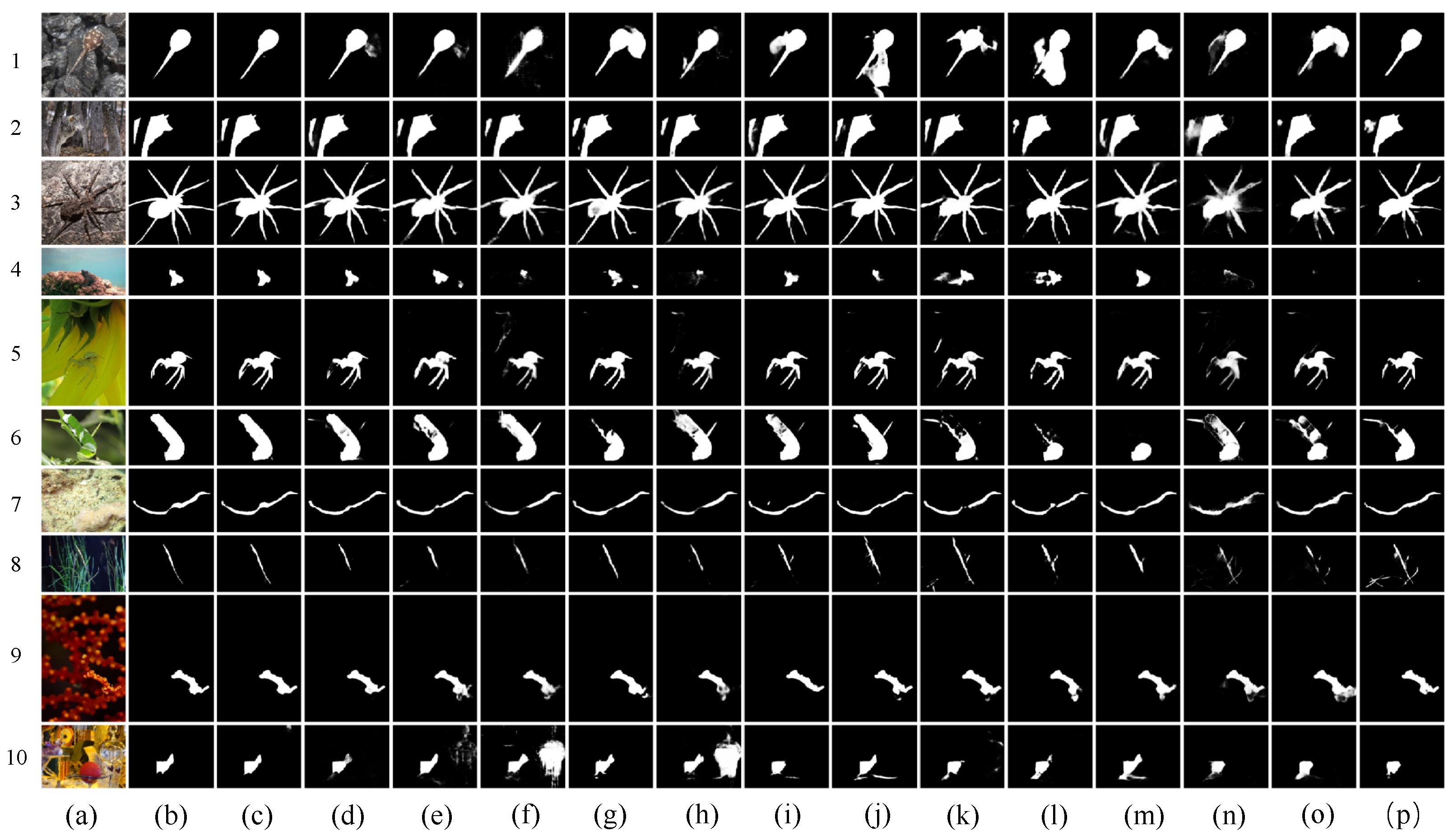
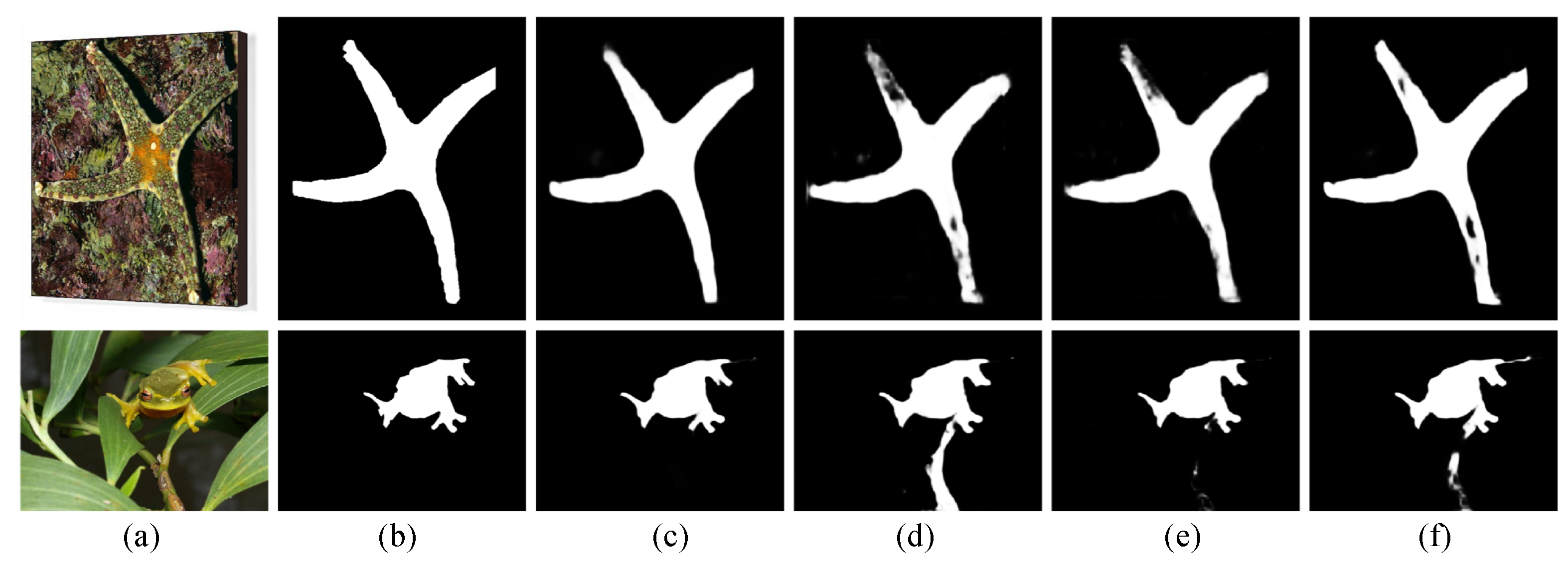
Our model’s results are more similar to GT, as shown in Figure 4. This figure summarizes the qualitative comparisons we conducted for all models using various visual contrast experiments. In other words, our results are more comprehensive and accurate compared to other models. Overall, our model has two significant advantages. Our model is capable of improving the edge information of large objects, as shown in the first, second, third, fifth, and sixth rows of Figure 4. This is primarily due to the UFM module, which effectively filters interference and distinguishes between the foreground and background by thoroughly mining low-level information. Our model can accurately segment small camouflaged objects, as shown in the fourth, seventh, eighth, ninth, and tenth rows of Figure 4. This is because we gradually fuse low-level and high-level features using the NFFM and top-down strategy, resulting in accurate prediction maps.
Based on the aforementioned comparison, we can conclusively demonstrate the superiority of FLCNet. Whether identifying small objects or edge features, our model outperforms existing methods in COD.
4.4. Comparisons of Inference
We also compare our model with other methods in terms of parameters (Params), floating point operations (FLOPs), and frames per second (FPS), as shown in Table 3. While our model produced positive results, the inference structure’s architecture still contains some redundant elements. We want to emphasize that by including UFM and NFFM modules, our method outperformed the comparison methods, striking a compromise between model complexity and performance. This shows that the primary goal of this work has been achieved. For future work, we will explore and improve our approach by considering integrated solutions for accuracy and efficiency, as well as addressing the increased inference cost consumption.
4.5. Ablation Studies
The effectiveness of the proposed UFM and NFFM is demonstrated in this section through our ablation studies on three COD datasets. Quantitative and qualitative comparisons are shown in Table 4 and Figure 5.
Table 4 illustrates how each module improves the model’s performance, with the best results achieved when all suggested modules are combined. Adding UFM or NFFM to the basic structure results in gradual increases in the evaluation scores across all three datasets, particularly in terms of the . Our model’s scores increased by 8.97%, 15.00%, and 11.54% compared to the basic model, respectively. In addition, the 2nd and 3rd rows in Table 4 show the two suggested modules significantly enhance the model’s performance compared to the basic model. The NFFM module has the most significant impact on MAE performance, increasing it by 7.69%, 12.50%, and 11.54% in the three datasets, compared to the basic module.
We also provide the prediction maps for each ablation experiment, demonstrating the effectiveness of our suggested modules. Figure 5 shows that UFM distinguishes between the foreground and background by mining low-level information, thus improving the resolution of edge information. Meanwhile, the NFFM and top-down strategy gradually fuse low-level features with high-level features to accurately locate the target location and generate an accurate predicted map.
Based on both qualitative comparisons and quantitative comparisons of the ablation investigation, it is clear that our model fully conforms to anticipated design standards and demonstrates a superior performance.
4.6. Failure Cases and Analysis
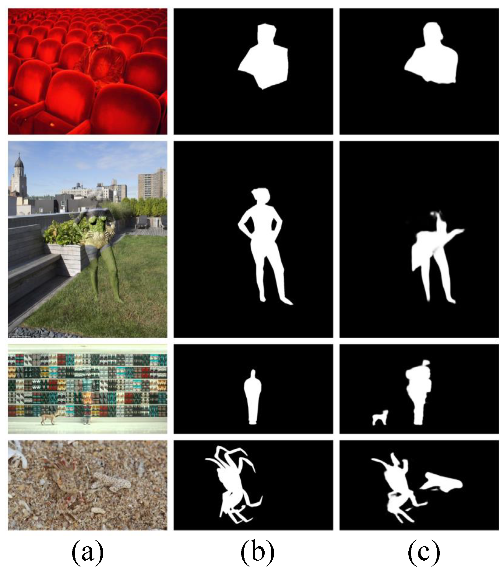
Based on the previous findings, our model still has some drawbacks, even though it performs better overall than other models. As shown in Figure 6, we display some scenarios where it fails. Detecting highly intricate artificial camouflage was not particularly successful using our methodology. As seen in first, second, and third rows of figures, the background and objects combined seamlessly, making it impossible for our algorithm to infer boundaries accurately. This issue could be due to the insufficient depth of mining and poor usage of edge detail information. Meanwhile, when an image contains both salient objects and camouflaged objects, our model can become confused and mistakenly segment the salient objects as camouflaged objects. As seen in the third and fourth rows, containing objects of two categories, the model has identified the objects. However, salient objects generally stand out significantly from the background, whereas a camouflaged object differs only slightly. This suggests that feature extraction and refinement alone will not enable the model to discern the differences between the two. Meanwhile, in our model, ReLU was mainly used as the activation function. In future research, we will consider using adaptive activation functions, which have a better learning ability than fixed activations and can greatly improve the convergence speed and increase model accuracy [47,48,49,50]. This also provides new directions for future improvements.
5. Conclusions
We introduce a new model named FLCNet, which comprises a UFM, a TEM, and an NFFM. The proposed UFM addresses the problem of existing models ignoring the deep exploration of low-level features, while the proposed NFFM avoids the problem of low efficiency in cross-level feature fusion. Finally, we use a top-down strategy to gradually integrate high-level and low-level features to generate an accurately predicted map. Through a series of comparison and ablation experiments, we have demonstrated the effectiveness and superiority of our model. However, our model still has some limitations, as it is not particularly successful at detecting highly complex artificial camouflage. At the same time, our model cannot distinguish salient objects from camouflaged objects. In the following research, we will further optimize this issue. Additionally, we hope that our model can be applied to more fields, such as polyp detection, steel defect detection, etc.
Author Contributions
Methodology, T.W.; software, R.W.; supervision, J.W.; writing—original draft, T.W.; writing—review and editing, T.W. and J.W. All authors have read and agreed to the published version of the manuscript.
Funding
This research received no external funding.
Data Availability Statement
The data will be available at https://github.com/Tao-Wang-CV/FLCNet.
Conflicts of Interest
The authors declare no conflict of interest.
References
- Lv, Y.; Zhang, J.; Dai, Y.; Li, A.; Liu, B.; Barnes, N.; Fan, D.P. Simultaneously localize, segment and rank the camouflaged objects. In Proceedings of the IEEE/CVF Conference on Computer Vision and Pattern Recognition, Nashville, TN, USA, 18–22 June 2021; pp. 11591–11601. [Google Scholar]
- Mei, H.; Ji, G.P.; Wei, Z.; Yang, X.; Wei, X.; Fan, D.P. Camouflaged object segmentation with distraction mining. In Proceedings of the IEEE/CVF Conference on Computer Vision and Pattern Recognition, Nashville, TN, USA, 18–22 June 2021; pp. 8772–8781. [Google Scholar]
- Zhou, T.; Zhou, Y.; Gong, C.; Yang, J.; Zhang, Y. Feature Aggregation and Propagation Network for Camouflaged Object Detection. IEEE Trans. Image Process. 2022, 31, 7036–7047. [Google Scholar] [CrossRef]
- Pang, Y.; Zhao, X.; Zhang, L.; Lu, H. Multi-scale interactive network for salient object detection. In Proceedings of the IEEE/CVF Conference on Computer Vision and Pattern Recognition, Seattle, WA, USA, 13–19 June 2020; pp. 9413–9422. [Google Scholar]
- Le, X.; Mei, J.; Zhang, H.; Zhou, B.; Xi, J. A learning-based approach for surface defect detection using small image datasets. Neurocomputing 2020, 408, 112–120. [Google Scholar] [CrossRef]
- Lidbetter, T. Search and rescue in the face of uncertain threats. Eur. J. Oper. Res. 2020, 285, 1153–1160. [Google Scholar] [CrossRef] [Green Version]
- Zhang, X.; Zhu, C.; Wang, S.; Liu, Y.; Ye, M. A Bayesian approach to camouflaged moving object detection. IEEE Trans. Circuits Syst. Video Technol. 2016, 27, 2001–2013. [Google Scholar] [CrossRef]
- Feng, X.; Guoying, C.; Richang, H.; Jing, G. Camouflage texture evaluation using a saliency map. Multimed. Syst. 2015, 21, 169–175. [Google Scholar] [CrossRef]
- Tankus, A.; Yeshurun, Y. Detection of regions of interest and camouflage breaking by direct convexity estimation. In Proceedings of the 1998 IEEE Workshop on Visual Surveillance, Bombay, India, 2 January 1998; pp. 42–48. [Google Scholar]
- Guo, H.; Dou, Y.; Tian, T.; Zhou, J.; Yu, S. A robust foreground segmentation method by temporal averaging multiple video frames. In Proceedings of the 2008 International Conference on Audio, Language and Image Processing, Shanghai, China, 7–9 July 2008; pp. 878–882. [Google Scholar]
- Fan, D.P.; Ji, G.P.; Cheng, M.M.; Shao, L. Concealed object detection. IEEE Trans. Pattern Anal. Mach. Intell. 2021, 44, 6024. [Google Scholar] [CrossRef]
- Yang, F.; Zhai, Q.; Li, X.; Huang, R.; Luo, A.; Cheng, H.; Fan, D.P. Uncertainty-guided transformer reasoning for camouflaged object detection. In Proceedings of the IEEE/CVF International Conference on Computer Vision, Nashville, TN, USA, 18–22 June 2021; pp. 4146–4155. [Google Scholar]
- Sun, Y.; Chen, G.; Zhou, T.; Zhang, Y.; Liu, N. Context-aware cross-level fusion network for camouflaged object detection. arXiv 2021, arXiv:2105.12555. [Google Scholar]
- Zhai, Q.; Li, X.; Yang, F.; Chen, C.; Cheng, H.; Fan, D.P. Mutual graph learning for camouflaged object detection. In Proceedings of the IEEE/CVF Conference on Computer Vision and Pattern Recognition, Nashville, TN, USA, 18–22 June 2021; pp. 12997–13007. [Google Scholar]
- Wu, Z.; Su, L.; Huang, Q. Cascaded partial decoder for fast and accurate salient object detection. In Proceedings of the IEEE/CVF Conference on Computer Vision and Pattern Recognition, Long Beach, CA, USA, 15–20 June 2019; pp. 3907–3916. [Google Scholar]
- Le, T.N.; Nguyen, T.V.; Nie, Z.; Tran, M.T.; Sugimoto, A. Anabranch network for camouflaged object segmentation. Comput. Vis. Image Underst. 2019, 184, 45–56. [Google Scholar] [CrossRef]
- Skurowski, P.; Abdulameer, H.; Błaszczyk, J.; Depta, T.; Kornacki, A.; Kozieł, P. Animal camouflage analysis: Chameleon database. Unpubl. Manuscr. 2018, 2, 7. [Google Scholar]
- Itti, L.; Koch, C.; Niebur, E. A model of saliency-based visual attention for rapid scene analysis. IEEE Trans. Pattern Anal. Mach. Intell. 1998, 20, 1254–1259. [Google Scholar] [CrossRef] [Green Version]
- Fang, H.; Gupta, S.; Iandola, F.; Srivastava, R.K.; Deng, L.; Dollár, P.; Gao, J.; He, X.; Mitchell, M.; Platt, J.C.; et al. From captions to visual concepts and back. In Proceedings of the IEEE Conference on Computer Vision and Pattern Recognition, Boston, MA, USA, 7–12 June 2015; pp. 1473–1482. [Google Scholar]
- Liu, N.; Han, J.; Yang, M.H. Picanet: Learning pixel-wise contextual attention for saliency detection. In Proceedings of the IEEE Conference on Computer Vision and Pattern Recognition, Salt Lake City, UT, USA, 18–23 June 2018; pp. 3089–3098. [Google Scholar]
- Ronneberger, O.; Fischer, P.; Brox, T. U-net: Convolutional networks for biomedical image segmentation. In Proceedings of the International Conference on Medical Image Computing and Computer-Assisted Intervention, Munich, Germany, 5–9 October 2015; pp. 234–241. [Google Scholar]
- Zhang, X.; Wang, T.; Qi, J.; Lu, H.; Wang, G. Progressive attention guided recurrent network for salient object detection. In Proceedings of the IEEE Conference on Computer Vision and Pattern Recognition, Salt Lake City, UT, USA, 18–23 June 2018; pp. 714–722. [Google Scholar]
- Wang, B.; Chen, Q.; Zhou, M.; Zhang, Z.; Jin, X.; Gai, K. Progressive feature polishing network for salient object detection. In Proceedings of the AAAI Conference on Artificial Intelligence, New York, NY, USA, 7–12 February 2020; Volume 34, pp. 12128–12135. [Google Scholar]
- Fan, D.P.; Ji, G.P.; Sun, G.; Cheng, M.M.; Shen, J.; Shao, L. Camouflaged object detection. In Proceedings of the IEEE/CVF Conference on Computer Vision and Pattern Recognition, Seattle, WA, USA, 13–19 June 2020; pp. 2777–2787. [Google Scholar]
- Li, A.; Zhang, J.; Lv, Y.; Liu, B.; Zhang, T.; Dai, Y. Uncertainty-aware joint salient object and camouflaged object detection. In Proceedings of the IEEE/CVF Conference on Computer Vision and Pattern Recognition, Nashville, TN, USA, 18–22 June 2021; pp. 10071–10081. [Google Scholar]
- Gao, S.H.; Cheng, M.M.; Zhao, K.; Zhang, X.Y.; Yang, M.H.; Torr, P. Res2net: A new multi-scale backbone architecture. IEEE Trans. Pattern Anal. Mach. Intell. 2019, 43, 652–662. [Google Scholar] [CrossRef] [PubMed] [Green Version]
- Dobzhansky, T. Nothing in biology makes sense except in the light of evolution. Am. Biol. Teach. 2013, 75, 87–91. [Google Scholar] [CrossRef]
- Fan, D.P.; Ji, G.P.; Qin, X.; Cheng, M.M. Cognitive vision inspired object segmentation metric and loss function. Sci. Sin. Inform. 2021, 6, 6. [Google Scholar]
- Qin, X.; Zhang, Z.; Huang, C.; Gao, C.; Dehghan, M.; Jagersand, M. Basnet: Boundary-aware salient object detection. In Proceedings of the IEEE/CVF Conference on Computer Vision and Pattern Recognition, Long Beach, CA, USA, 15–20 June 2019; pp. 7479–7489. [Google Scholar]
- De Boer, P.T.; Kroese, D.P.; Mannor, S.; Rubinstein, R.Y. A tutorial on the cross-entropy method. Ann. Oper. Res. 2005, 134, 19–67. [Google Scholar] [CrossRef]
- Wei, J.; Wang, S.; Huang, Q. F3Net: Fusion, feedback and focus for salient object detection. In Proceedings of the AAAI Conference on Artificial Intelligence, New York, NY, USA, 7–12 February 2020; Volume 34, pp. 12321–12328. [Google Scholar]
- Da, K. A method for stochastic optimization. arXiv 2014, arXiv:1412.6980. [Google Scholar]
- Fan, D.P.; Cheng, M.M.; Liu, Y.; Li, T.; Borji, A. Structure-measure: A new way to evaluate foreground maps. In Proceedings of the IEEE International Conference on Computer Vision, Venice, Italy, 22–29 October 2017; pp. 4548–4557. [Google Scholar]
- Margolin, R.; Zelnik-Manor, L.; Tal, A. How to evaluate foreground maps? In Proceedings of the IEEE Conference on Computer Vision and Pattern Recognition, Columbus, OH, USA, 23–28 June 2014; pp. 248–255. [Google Scholar]
- Achanta, R.; Hemami, S.; Estrada, F.; Susstrunk, S. Frequency-tuned salient region detection. In Proceedings of the 2009 IEEE Conference on Computer Vision and Pattern Recognition, Miami, FL, USA, 20–25 June 2009; pp. 1597–1604. [Google Scholar]
- Fan, D.P.; Gong, C.; Cao, Y.; Ren, B.; Cheng, M.M.; Borji, A. Enhanced-alignment measure for binary foreground map evaluation. arXiv 2018, arXiv:1805.10421. [Google Scholar]
- Zhang, D.; Han, J.; Li, C.; Wang, J.; Li, X. Detection of co-salient objects by looking deep and wide. Int. J. Comput. Vis. 2016, 120, 215–232. [Google Scholar] [CrossRef]
- Zhao, J.X.; Liu, J.J.; Fan, D.P.; Cao, Y.; Yang, J.; Cheng, M.M. EGNet: Edge guidance network for salient object detection. In Proceedings of the IEEE/CVF International Conference on Computer Vision, Seoul, Republic of Korea, 27 October–2 November 2019; pp. 8779–8788. [Google Scholar]
- Wu, Z.; Su, L.; Huang, Q. Stacked cross refinement network for edge-aware salient object detection. In Proceedings of the IEEE/CVF International Conference on Computer Vision, Seoul, Republic of Korea, 27 October–2 November 2019; pp. 7264–7273. [Google Scholar]
- Liu, J.J.; Hou, Q.; Cheng, M.M.; Feng, J.; Jiang, J. A simple pooling-based design for real-time salient object detection. In Proceedings of the IEEE/CVF Conference on Computer Vision and Pattern Recognition, Long Beach, CA, USA, 15–20 June 2019; pp. 3917–3926. [Google Scholar]
- Gao, S.H.; Tan, Y.Q.; Cheng, M.M.; Lu, C.; Chen, Y.; Yan, S. Highly efficient salient object detection with 100k parameters. In Proceedings of the European Conference on Computer Vision, Glasgow, UK, 8–14 September 2020; pp. 702–721. [Google Scholar]
- Zhang, J.; Yu, X.; Li, A.; Song, P.; Liu, B.; Dai, Y. Weakly-supervised salient object detection via scribble annotations. In Proceedings of the IEEE/CVF Conference on Computer Vision and Pattern Recognition, Seattle, WA, USA, 13–19 June 2020; pp. 12546–12555. [Google Scholar]
- Zhang, J.; Fan, D.P.; Dai, Y.; Anwar, S.; Saleh, F.S.; Zhang, T.; Barnes, N. UC-Net: Uncertainty inspired RGB-D saliency detection via conditional variational autoencoders. In Proceedings of the IEEE/CVF Conference on Computer Vision and Pattern Recognition, Seattle, WA, USA, 13–19 June 2020; pp. 8582–8591. [Google Scholar]
- Zhou, H.; Xie, X.; Lai, J.H.; Chen, Z.; Yang, L. Interactive two-stream decoder for accurate and fast saliency detection. In Proceedings of the IEEE/CVF Conference on Computer Vision and Pattern Recognition, Seattle, WA, USA, 13–19 June 2020; pp. 9141–9150. [Google Scholar]
- Fan, D.P.; Ji, G.P.; Zhou, T.; Chen, G.; Fu, H.; Shen, J.; Shao, L. Pranet: Parallel reverse attention network for polyp segmentation. In Proceedings of the International Conference on Medical Image Computing and Computer-Assisted Intervention, Lima, Peru, 4–8 October 2020; pp. 263–273. [Google Scholar]
- Yan, J.; Le, T.N.; Nguyen, K.D.; Tran, M.T.; Do, T.T.; Nguyen, T.V. Mirrornet: Bio-inspired camouflaged object segmentation. IEEE Access 2021, 9, 43290–43300. [Google Scholar] [CrossRef]
- Jagtap, A.D.; Kawaguchi, K.; Karniadakis, G.E. Adaptive activation functions accelerate convergence in deep and physics-informed neural networks. J. Comput. Phys. 2020, 404, 109136. [Google Scholar] [CrossRef] [Green Version]
- Jagtap, A.D.; Kawaguchi, K.; Em Karniadakis, G. Locally adaptive activation functions with slope recovery for deep and physics-informed neural networks. Proc. R. Soc. A 2020, 476, 20200334. [Google Scholar] [CrossRef]
- Jagtap, A.D.; Karniadakis, G.E. How important are activation functions in regression and classification? A survey, performance comparison, and future directions. J. Mach. Learn. Model. Comput. 2023, 4, 21–75. [Google Scholar] [CrossRef]
- Jagtap, A.D.; Shin, Y.; Kawaguchi, K.; Karniadakis, G.E. Deep Kronecker neural networks: A general framework for neural networks with adaptive activation functions. Neurocomputing 2022, 468, 165–180. [Google Scholar] [CrossRef]
Figure 1.
Examples of camouflaged objects. (a) Camouflaged object, (b) GT.

Figure 2.
The overall architecture of the proposed FLCNet, which includes three key components, an underlying feature mining module (UFM), a texture-enhanced module (TEM), and a neighborhood feature fusion module (NFFM). The input is , and the result is a prediction map .
Figure 2.
The overall architecture of the proposed FLCNet, which includes three key components, an underlying feature mining module (UFM), a texture-enhanced module (TEM), and a neighborhood feature fusion module (NFFM). The input is , and the result is a prediction map .
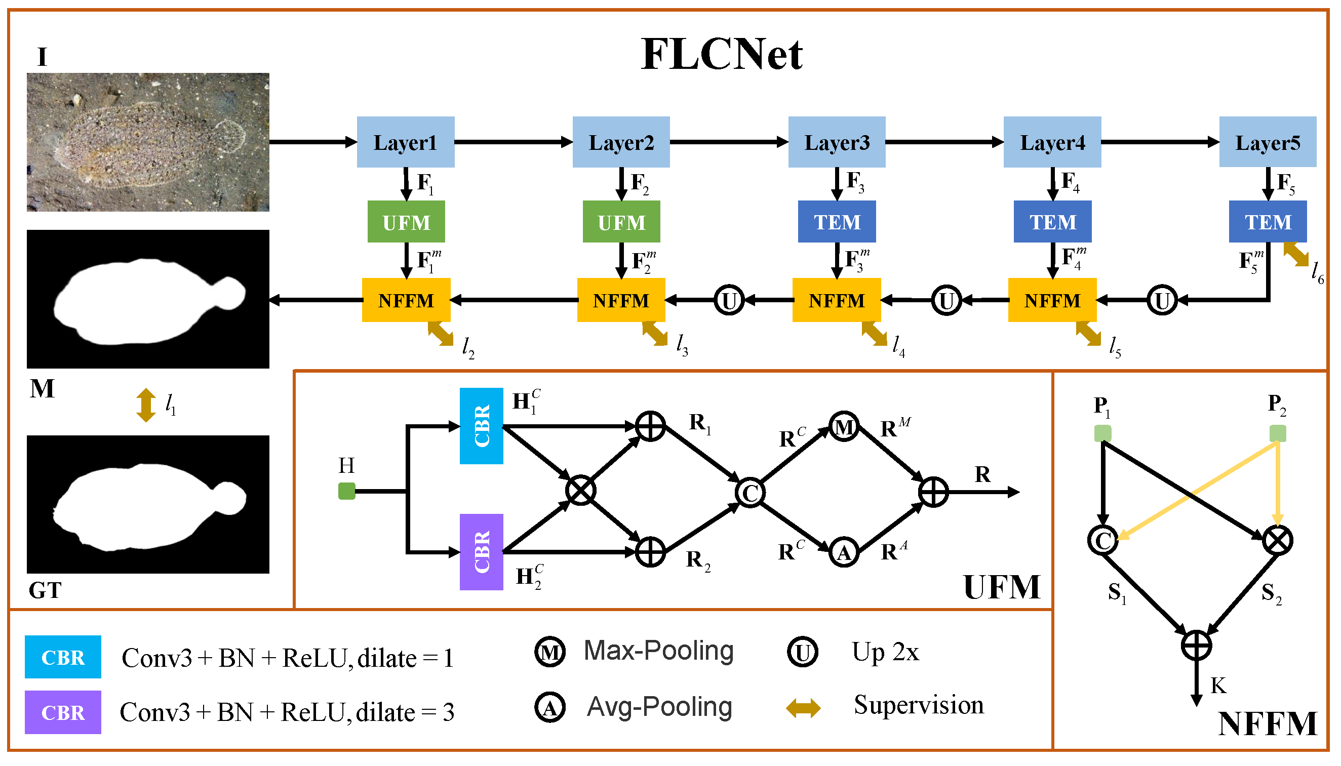
Figure 3.
Quantitative evaluation of different models. (a) shows CHAMELEONs Recall, (b) shows CHAMELEONs threshold.
Figure 3.
Quantitative evaluation of different models. (a) shows CHAMELEONs Recall, (b) shows CHAMELEONs threshold.
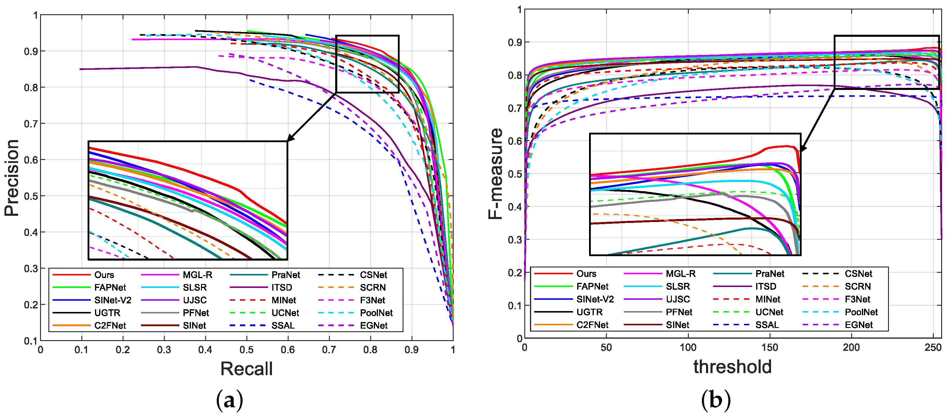
Figure 4.
Visual comparison of our and other models on four COD testing datasets. (a) Input, (b) GT, (c) Ours, (d) FAPNet [3] (e) SINet_V2 [11], (f) UGTR [12], (g) C2FNet [13], (h) MGL-R [14], (i) SLSR [1], (j) UJSC [25], (k) PFNet [2], (l) SINet [24], (m) PraNet [45], (n) ITSD [44], (o) MINet [4], (p) UCNet [43].

Figure 5.
Qualitative comparisons of our model. (a) Input, (b) GT, (c) Ours, (d) Basic, (e) Basic+UFM, (f) Basic+NFFM.
Figure 5.
Qualitative comparisons of our model. (a) Input, (b) GT, (c) Ours, (d) Basic, (e) Basic+UFM, (f) Basic+NFFM.

Figure 6.
Some failed examples. (a) Input, (b) GT, (c) Ours.


Table 1.
Quantitative comparison of different methods on four COD testing datasets. Here, “↑” (“↓”) means that the larger (smaller) the better. The best three results in each column are marked in red, green, and blue.
Table 1.
Quantitative comparison of different methods on four COD testing datasets. Here, “↑” (“↓”) means that the larger (smaller) the better. The best three results in each column are marked in red, green, and blue.
| CAMO Dataset | CHAMELEON Dataset | COD10K Dataset | NC4K Dataset | |||||||||||||||||
|---|---|---|---|---|---|---|---|---|---|---|---|---|---|---|---|---|---|---|---|---|
| EGNet [38] | 0.732 | 0.604 | 0.670 | 0.800 | 0.109 | 0.797 | 0.649 | 0.702 | 0.860 | 0.065 | 0.736 | 0.517 | 0.582 | 0.810 | 0.061 | 0.777 | 0.639 | 0.696 | 0.841 | 0.075 |
| PoolNet [40] | 0.730 | 0.575 | 0.643 | 0.747 | 0.105 | 0.845 | 0.691 | 0.749 | 0.864 | 0.054 | 0.740 | 0.506 | 0.576 | 0.777 | 0.056 | 0.785 | 0.635 | 0.699 | 0.814 | 0.073 |
| F3Net [31] | 0.711 | 0.564 | 0.616 | 0.741 | 0.109 | 0.848 | 0.744 | 0.770 | 0.894 | 0.047 | 0.739 | 0.544 | 0.593 | 0.795 | 0.051 | 0.780 | 0.656 | 0.705 | 0.824 | 0.070 |
| SCRN [39] | 0.779 | 0.643 | 0.705 | 0.797 | 0.090 | 0.876 | 0.741 | 0.787 | 0.889 | 0.042 | 0.789 | 0.575 | 0.651 | 0.817 | 0.047 | 0.830 | 0.698 | 0.757 | 0.854 | 0.059 |
| CSNet [41] | 0.771 | 0.642 | 0.705 | 0.795 | 0.092 | 0.856 | 0.718 | 0.766 | 0.869 | 0.047 | 0.778 | 0.569 | 0.635 | 0.810 | 0.047 | 0.750 | 0.603 | 0.655 | 0.773 | 0.088 |
| SSAL [42] | 0.644 | 0.493 | 0.579 | 0.721 | 0.126 | 0.757 | 0.639 | 0.702 | 0.849 | 0.071 | 0.668 | 0.454 | 0.527 | 0.768 | 0.066 | 0.699 | 0.561 | 0.644 | 0.780 | 0.093 |
| UCNet [43] | 0.739 | 0.640 | 0.700 | 0.787 | 0.094 | 0.880 | 0.817 | 0.836 | 0.930 | 0.036 | 0.776 | 0.633 | 0.681 | 0.857 | 0.042 | 0.811 | 0.729 | 0.775 | 0.871 | 0.055 |
| MINet [4] | 0.748 | 0.637 | 0.691 | 0.792 | 0.090 | 0.855 | 0.771 | 0.802 | 0.914 | 0.036 | 0.770 | 0.608 | 0.657 | 0.832 | 0.042 | 0.812 | 0.720 | 0.764 | 0.862 | 0.056 |
| ITSD [44] | 0.750 | 0.610 | 0.663 | 0.780 | 0.102 | 0.814 | 0.662 | 0.705 | 0.844 | 0.057 | 0.767 | 0.557 | 0.615 | 0.808 | 0.051 | 0.811 | 0.680 | 0.729 | 0.845 | 0.064 |
| PraNet [45] | 0.769 | 0.663 | 0.710 | 0.824 | 0.094 | 0.860 | 0.763 | 0.789 | 0.907 | 0.044 | 0.789 | 0.629 | 0.671 | 0.861 | 0.045 | 0.822 | 0.724 | 0.762 | 0.876 | 0.059 |
| ANet [16] | 0.682 | 0.484 | 0.541 | 0.685 | 0.126 | - | - | - | - | - | - | - | - | - | - | - | - | - | - | - |
| MirrorNet [46] | 0.785 | 0.719 | 0.754 | 0.848 | 0.077 | - | - | - | - | - | - | - | - | - | - | - | - | - | - | - |
| SINet [24] | 0.745 | 0.644 | 0.702 | 0.804 | 0.092 | 0.872 | 0.806 | 0.827 | 0.936 | 0.034 | 0.776 | 0.631 | 0.679 | 0.864 | 0.043 | 0.808 | 0.723 | 0.769 | 0.871 | 0.058 |
| PFNet [2] | 0.782 | 0.695 | 0.746 | 0.842 | 0.085 | 0.882 | 0.810 | 0.828 | 0.931 | 0.033 | 0.800 | 0.660 | 0.701 | 0.877 | 0.040 | 0.829 | 0.745 | 0.784 | 0.888 | 0.053 |
| UJSC [25] | 0.800 | 0.728 | 0.772 | 0.859 | 0.073 | 0.891 | 0.833 | 0.847 | 0.945 | 0.030 | 0.809 | 0.684 | 0.721 | 0.884 | 0.035 | 0.842 | 0.771 | 0.806 | 0.898 | 0.047 |
| SLSR [1] | 0.787 | 0.696 | 0.744 | 0.838 | 0.080 | 0.890 | 0.822 | 0.841 | 0.935 | 0.030 | 0.804 | 0.673 | 0.715 | 0.880 | 0.037 | 0.840 | 0.766 | 0.804 | 0.895 | 0.048 |
| MGL-R [14] | 0.775 | 0.673 | 0.726 | 0.812 | 0.088 | 0.893 | 0.813 | 0.834 | 0.918 | 0.030 | 0.814 | 0.666 | 0.711 | 0.852 | 0.035 | 0.833 | 0.740 | 0.782 | 0.867 | 0.052 |
| C2FNet [13] | 0.796 | 0.719 | 0.762 | 0.854 | 0.080 | 0.888 | 0.828 | 0.844 | 0.935 | 0.032 | 0.813 | 0.686 | 0.723 | 0.890 | 0.036 | 0.838 | 0.762 | 0.795 | 0.897 | 0.049 |
| UGTR [12] | 0.784 | 0.684 | 0.736 | 0.822 | 0.086 | 0.887 | 0.794 | 0.820 | 0.910 | 0.031 | 0.817 | 0.666 | 0.711 | 0.853 | 0.036 | 0.839 | 0.747 | 0.787 | 0.875 | 0.052 |
| SINet_V2 [11] | 0.820 | 0.743 | 0.782 | 0.882 | 0.070 | 0.888 | 0.816 | 0.835 | 0.942 | 0.030 | 0.815 | 0.680 | 0.718 | 0.887 | 0.037 | 0.847 | 0.770 | 0.805 | 0.903 | 0.048 |
| FAPNet [3] | 0.815 | 0.734 | 0.776 | 0.865 | 0.076 | 0.893 | 0.825 | 0.842 | 0.940 | 0.028 | 0.822 | 0.694 | 0.731 | 0.888 | 0.036 | 0.851 | 0.775 | 0.810 | 0.899 | 0.047 |
| Ours | 0.808 | 0.741 | 0.782 | 0.873 | 0.071 | 0.891 | 0.837 | 0.851 | 0.948 | 0.028 | 0.818 | 0.700 | 0.734 | 0.893 | 0.034 | 0.845 | 0.780 | 0.813 | 0.905 | 0.046 |
Table 2.
Quantitative comparison of different methods on four COD10K testing dataset categories. Here, “↑” (“↓”) means that the larger (smaller) the better. The best three results in each column are marked in red, green, and blue.
Table 2.
Quantitative comparison of different methods on four COD10K testing dataset categories. Here, “↑” (“↓”) means that the larger (smaller) the better. The best three results in each column are marked in red, green, and blue.
| COD10K-Amphibian | COD10K-Aquatic | COD10K-Flying | COD10K-Terrestrial | |||||||||||||||||
|---|---|---|---|---|---|---|---|---|---|---|---|---|---|---|---|---|---|---|---|---|
| EGNet [38] | 0.776 | 0.588 | 0.650 | 0.843 | 0.056 | 0.712 | 0.515 | 0.584 | 0.784 | 0.091 | 0.769 | 0.558 | 0.621 | 0.838 | 0.046 | 0.713 | 0.467 | 0.531 | 0.794 | 0.056 |
| PoolNet [40] | 0.781 | 0.584 | 0.644 | 0.823 | 0.050 | 0.737 | 0.534 | 0.607 | 0.782 | 0.078 | 0.767 | 0.539 | 0.610 | 0.797 | 0.045 | 0.707 | 0.441 | 0.508 | 0.745 | 0.054 |
| F3Net [31] | 0.808 | 0.657 | 0.700 | 0.846 | 0.039 | 0.728 | 0.554 | 0.611 | 0.788 | 0.076 | 0.760 | 0.571 | 0.618 | 0.818 | 0.040 | 0.712 | 0.490 | 0.538 | 0.770 | 0.048 |
| SCRN [39] | 0.839 | 0.665 | 0.729 | 0.867 | 0.041 | 0.780 | 0.600 | 0.674 | 0.818 | 0.064 | 0.817 | 0.608 | 0.683 | 0.840 | 0.036 | 0.758 | 0.509 | 0.588 | 0.784 | 0.048 |
| CSNet [41] | 0.828 | 0.649 | 0.711 | 0.857 | 0.041 | 0.768 | 0.587 | 0.656 | 0.808 | 0.067 | 0.809 | 0.610 | 0.676 | 0.838 | 0.036 | 0.744 | 0.501 | 0.566 | 0.776 | 0.047 |
| SSAL [42] | 0.729 | 0.560 | 0.637 | 0.817 | 0.057 | 0.632 | 0.428 | 0.509 | 0.737 | 0.101 | 0.702 | 0.504 | 0.576 | 0.795 | 0.050 | 0.647 | 0.405 | 0.471 | 0.756 | 0.060 |
| UCNet [43] | 0.827 | 0.717 | 0.756 | 0.897 | 0.034 | 0.767 | 0.649 | 0.703 | 0.843 | 0.060 | 0.806 | 0.675 | 0.718 | 0.886 | 0.030 | 0.742 | 0.566 | 0.617 | 0.830 | 0.042 |
| MINet [4] | 0.823 | 0.695 | 0.732 | 0.881 | 0.035 | 0.767 | 0.632 | 0.684 | 0.831 | 0.058 | 0.799 | 0.650 | 0.697 | 0.856 | 0.031 | 0.732 | 0.536 | 0.584 | 0.802 | 0.043 |
| ITSD [44] | 0.810 | 0.628 | 0.679 | 0.852 | 0.044 | 0.762 | 0.584 | 0.648 | 0.811 | 0.070 | 0.793 | 0.588 | 0.645 | 0.831 | 0.040 | 0.736 | 0.496 | 0.552 | 0.777 | 0.051 |
| PraNet [45] | 0.842 | 0.717 | 0.750 | 0.905 | 0.035 | 0.781 | 0.643 | 0.692 | 0.848 | 0.065 | 0.819 | 0.669 | 0.707 | 0.888 | 0.033 | 0.756 | 0.565 | 0.607 | 0.835 | 0.046 |
| ANet [16] | - | - | - | - | - | - | - | - | - | - | - | - | - | - | - | - | - | - | - | - |
| MirrorNet [46] | - | - | - | - | - | - | - | - | - | - | - | - | - | - | - | - | - | - | - | - |
| SINet [24] | 0.820 | 0.714 | 0.756 | 0.891 | 0.034 | 0.766 | 0.643 | 0.698 | 0.854 | 0.063 | 0.803 | 0.663 | 0.707 | 0.887 | 0.031 | 0.749 | 0.577 | 0.625 | 0.845 | 0.042 |
| PFNet [2] | 0.848 | 0.740 | 0.775 | 0.911 | 0.031 | 0.793 | 0.675 | 0.722 | 0.868 | 0.055 | 0.824 | 0.691 | 0.729 | 0.903 | 0.030 | 0.773 | 0.606 | 0.647 | 0.855 | 0.040 |
| UJSC [25] | 0.841 | 0.742 | 0.769 | 0.905 | 0.031 | 0.805 | 0.705 | 0.747 | 0.879 | 0.049 | 0.836 | 0.719 | 0.752 | 0.906 | 0.026 | 0.778 | 0.624 | 0.664 | 0.863 | 0.037 |
| SLSR [1] | 0.845 | 0.751 | 0.783 | 0.906 | 0.030 | 0.803 | 0.694 | 0.740 | 0.875 | 0.052 | 0.830 | 0.707 | 0.745 | 0.906 | 0.026 | 0.772 | 0.611 | 0.655 | 0.855 | 0.038 |
| MGL-R [14] | 0.854 | 0.734 | 0.770 | 0.886 | 0.028 | 0.807 | 0.688 | 0.736 | 0.855 | 0.051 | 0.839 | 0.701 | 0.743 | 0.873 | 0.026 | 0.785 | 0.606 | 0.651 | 0.823 | 0.036 |
| C2FNet [13] | 0.849 | 0.752 | 0.779 | 0.899 | 0.030 | 0.807 | 0.700 | 0.741 | 0.882 | 0.052 | 0.840 | 0.724 | 0.759 | 0.914 | 0.026 | 0.783 | 0.627 | 0.664 | 0.872 | 0.037 |
| UGTR [12] | 0.857 | 0.738 | 0.774 | 0.896 | 0.029 | 0.810 | 0.686 | 0.734 | 0.855 | 0.050 | 0.843 | 0.699 | 0.744 | 0.873 | 0.026 | 0.789 | 0.606 | 0.653 | 0.823 | 0.036 |
| SINet_V2 [11] | 0.858 | 0.756 | 0.788 | 0.916 | 0.030 | 0.811 | 0.696 | 0.738 | 0.883 | 0.051 | 0.839 | 0.713 | 0.749 | 0.908 | 0.027 | 0.787 | 0.623 | 0.662 | 0.866 | 0.039 |
| FAPNet [3] | 0.854 | 0.752 | 0.783 | 0.914 | 0.032 | 0.821 | 0.717 | 0.757 | 0.887 | 0.049 | 0.845 | 0.725 | 0.760 | 0.906 | 0.025 | 0.795 | 0.639 | 0.678 | 0.868 | 0.037 |
| Ours | 0.863 | 0.776 | 0.803 | 0.925 | 0.028 | 0.817 | 0.725 | 0.764 | 0.895 | 0.048 | 0.844 | 0.733 | 0.763 | 0.913 | 0.024 | 0.785 | 0.638 | 0.675 | 0.869 | 0.037 |
Table 3.
Comparisons of the number of parameters, FLOPs, and FPS corresponding to COD methods. All evaluations follow the inference settings in the corresponding papers.
Table 3.
Comparisons of the number of parameters, FLOPs, and FPS corresponding to COD methods. All evaluations follow the inference settings in the corresponding papers.
| Method | Ours | FAPNet [3] | SINet_V2 [11] | UGTR [12] | C2FNet [13] | MGL-R [14] | SINet [24] | SLSR [1] | UJSC [25] | PFNet [2] |
|---|---|---|---|---|---|---|---|---|---|---|
| Params. | 31.554 M | 29.524 M | 26.976 M | 48.868 M | 28.411 M | 63.595 M | 48.947 M | 50.935 M | 217.982 M | 46.498 M |
| FLOPs | 43.435 G | 59.101 G | 24.481 G | 1.007 T | 26.167 G | 553.939 G | 38.757 G | 66.625 G | 112.341 G | 53.222 G |
| FPS | 34.013 | 28.476 | 38.948 | 15.446 | 36.941 | 12.793 | 34.083 | 32.547 | 18.246 | 29.175 |
Table 4.
Ablation studies on three testing datasets.
| Method | CAMO Dataset | COD10K Dataset | NC4K Dataset | ||||||||||||
|---|---|---|---|---|---|---|---|---|---|---|---|---|---|---|---|
| Basic | 0.797 | 0.712 | 0.757 | 0.861 | 0.078 | 0.800 | 0.660 | 0.698 | 0.878 | 0.040 | 0.832 | 0.749 | 0.785 | 0.893 | 0.052 |
| Basic+UFM | 0.804 | 0.728 | 0.774 | 0.865 | 0.076 | 0.814 | 0.685 | 0.725 | 0.883 | 0.036 | 0.841 | 0.765 | 0.803 | 0.894 | 0.049 |
| Basic+NFFM | 0.806 | 0.738 | 0.781 | 0.873 | 0.072 | 0.817 | 0.700 | 0.734 | 0.892 | 0.035 | 0.843 | 0.777 | 0.810 | 0.903 | 0.046 |
| Ours | 0.808 | 0.741 | 0.782 | 0.873 | 0.071 | 0.818 | 0.700 | 0.734 | 0.893 | 0.034 | 0.845 | 0.780 | 0.813 | 0.905 | 0.046 |
Disclaimer/Publisher’s Note: The statements, opinions and data contained in all publications are solely those of the individual author(s) and contributor(s) and not of MDPI and/or the editor(s). MDPI and/or the editor(s) disclaim responsibility for any injury to people or property resulting from any ideas, methods, instructions or products referred to in the content. |
© 2023 by the authors. Licensee MDPI, Basel, Switzerland. This article is an open access article distributed under the terms and conditions of the Creative Commons Attribution (CC BY) license (https://creativecommons.org/licenses/by/4.0/).
Share and Cite
MDPI and ACS Style
Wang, T.; Wang, J.; Wang, R. Camouflaged Object Detection with a Feature Lateral Connection Network. Electronics 2023, 12, 2570. https://doi.org/10.3390/electronics12122570
AMA Style
Wang T, Wang J, Wang R. Camouflaged Object Detection with a Feature Lateral Connection Network. Electronics. 2023; 12(12):2570. https://doi.org/10.3390/electronics12122570
Chicago/Turabian StyleWang, Tao, Jian Wang, and Ruihao Wang. 2023. "Camouflaged Object Detection with a Feature Lateral Connection Network" Electronics 12, no. 12: 2570. https://doi.org/10.3390/electronics12122570
Note that from the first issue of 2016, this journal uses article numbers instead of page numbers. See further details here.