Learing Sampling and Reconstruction Using Bregman Iteration for CS-MRI

Abstract

The purpose of compressed sensing magnetic resonance imaging (CS-MRI) is to reconstruct clear images using data from the Nyquist sampling space. By reducing the amount of sampling, MR imaging can be accelerated, thereby improving the efficiency of device data collection and increasing patient throughput. The two basic challenges in CS-MRI are designing sparse sampling masks and designing effective reconstruction algorithms. In order to be consistent with the analysis conclusion of CS theory, we propose a bi-level optimization model to optimize the sampling mask and the reconstruction network at the same time under the constraints of data terms. The proposed sampling sub-network is based on an additive gradient strategy. In our reconstructed subnet, we design a phase deep unfolding network based on the Bregman iterative algorithm to find the solution of constrained problems by solving a series of unconstrained problems. Experiments on two widely used MRI datasets show that our proposed model yields sub-sampling patterns and reconstruction models customized for training data, achieving state-of-the-art results in terms of quantitative metrics and visual quality.

1. Introduction

Magnetic resonance imaging (MRI) is an advanced biomedical imaging technique with the advantages of non-ionizing radiation and multi-tissue contrast. In MRI, the data sampled is a Fourier transform of the signal, and sampling is a time-consuming process. Keeping acquisition times short is important to ensure patient comfort and reduce motion artifacts. One solution is to recover MR images based on compressed sensing (CS) theory. Compressed sensing MRI breaks the Nyquist–Shannon sampling barrier and reconstructs MR images with fewer sampling data, which is an excellent way to speed up reconstruction, and the two key challenges in CS-MRI [1,2] are how to design sampling patterns and how to design reconstruction algorithms.

For sampling patterns, some popular modes in CS-MRI include skipped-line Cartesian [3], random uniform [4], and variable density (VD) [5], all of which are simple and have good performance when combined with reconstruction methods. Most of these sampling masks, designed according to the variable density probability density function, are based on a kind of experimental observation that it is better to sample when the frequencies should be denser. This is also helpful for image recovering. Another common strategy, the radial mask [6], uses certain information sampled from different angles to achieve oversampling of low-frequency parts while reducing shadows in image motion. However, the masks in these sampling schemes are heuristic and independently designed due to the need to consider the effects of specific data, as well as reconstruction algorithms. This leaves room for future improvement.

For an MRI reconstruction algorithm, theoretically, assuming that the data is sparse under a certain transformation domain, then, by nonlinear optimization of random under-sampled raw data, reconstruction can be achieved without degrading image quality.Traditional model-based MRI reconstruction has been extensively studied [7,8,9,10]. These methods usually design different regular terms, such as wavelets [11] or TV [12], using the method of iterative optimization [13]. The problem with such methods is that the reconstruction image is too smooth, and the calculation is complex and time-consuming.

Nowadays, in order to make full use of existing data, efficient data-driven methods are on the horizon. Some CS-based deep unfolding networks [14,15] (DUNs) have been developed, such as ISTA-Net, which is based on the traditional iterative shrinkage threshold algorithm (ISTA) and unfolds iterations into a network with a fixed number of stages, with each stage corresponding to one iteration in ISTA [15]. In addition, there has also been research [16,17] into the design of convolutional neural network structures to reconstruct MR images. U-NET [17] is widely known as a representative of the success of this approach and has good performance for medical images. Recent research has gradually paid more attention to finding different training goals, such as adversarial loss [18] and perceived loss [19], to improve recovery quality.

The above work treats sampling and reconstruction as two separate problems. However, the optimal under-sampling mask depends on the specific MRI reconstruction method, and a good sampling mask can improve the recovery quality of the reconstruction method. In this paper, we use a bi-level optimization method to deal with the above two problems, namely under-sampling and reconstruction, at the same time, to achieve an effective combination of sub-sampling learning and reconstructive network training. Specifically, based on the strategy of the accumulation gradient [20,21], we develop a sampling sub-network, learn the weight of each point, and decide whether to sample according to the size of the weight. Like PUERT [22], we adopt a dynamic gradient estimation strategy that progressively approximates the binarization function, which effectively preserves the gradient information and further improves the recovery quality. In order to be consistent with the conclusions of CS theory, our model is an optimization model with data term constraints. In order to deal with the constraint problem, we use a phase reconstruction network based on the Bregman [23] iterative algorithm to find the solution of the constraint problem by solving a series of unconstrained problems.

Overall, the main contributions of this paper are threefold.

A bi-level optimization model based on CS-MRI is proposed, and the sampling mask and reconstruction network are optimized at the same time.

The sampling subnet learns the weight of each sampling point, and obtains the sampling mask under different sampling ratios according to the size of the weight.

We propose a phase unfolding network based on the Bregman iterative algorithm to solve constraint optimization problems. Each stage of reconstructing the sub-network corresponds to solving an independent unconstrained problem, and as the network deepens, the residuals obtained from the training of the previous stage are added to the training of the network in the later stage, thereby encouraging the network to meet the solution of the constraint problem.

Related Work

In recent years, with the rapid development of deep learning, a series of learning-based models have been proposed [24,25,26,27,28,29,30]. DAGAN [30] features a sampling and full-image denoising network framework based on generative adversarial network (GAN [18]), which improves the performance of compressed perception image reconstruction by introducing adversarial loss and perceived loss. A joint deep model-based network for MR image and coil sensitivity reconstruction, called Joint IC-Net, was proposed in [31], which combines MR physical models to jointly reconstruct MR images and coil sensitivity maps from under-sampled multi-coil K-space data. There are also improved algorithms based on BM3D [32,33], which have also achieved good results.

LOUPE [34] and PUERT [22] both assume that each binary sampling element is an independent Bernoulli random variable and learn a probabilistic sampling pattern rather than a deterministic mask. PUERT introduces an effective gradient estimation strategy when using the binarization function, and uses DUN to make full use of the intrinsic structural features of mask knowledge at each stage to realize the combination of deep learning and traditional models. PUERT solves an unconstrained optimization problem (Equation (1))

$$u\left(S\right)=arg\underset{u}{min}\frac{1}{2}\left|\right|SFu-{Sy\left|\right|}_2^2+\lambda R\left(u\right).$$

(1)

LOUPE solves an optimization problem with sparsity constraints (Equation (2))

$$\begin{array}{cc}\hfill & \underset{S,\theta }{min}{E}_{S\sim {\prod }_{t=1}B\left({\sigma }_t\left(O_t\right)\right)}\sum _{i=1}^N\left|\right|A_{\theta }\left(F^{H}diag\left(S\right)F{u}_i\right)-u_i{\left|\right|}_2^2\hfill \\ \hfill & s.t.\frac{1}{d}\left|\right|{\sigma }_t\left(O\right){\left|\right|}_1=a.\hfill \end{array}$$

(2)

Compressed sensing theory [35] tells us that if the signal x is sparse under a certain transformation domain $\mathsf{\Psi }$, it is randomly sub-sampled, and if the observation matrix $\mathsf{\Phi }$ is not correlated with the sparse transformation base $\mathsf{\Psi }$, then the signal can be recovered by the following model (Equation (3))

$$\begin{array}{cc}\hfill & min{\left|\right|\mathsf{\Psi }x\left|\right|}_1\hfill \\ \hfill & s.t.\mathsf{\Phi }\mathsf{\Psi }x=y.\hfill \end{array}$$

(3)

In order to be consistent with the above theoretical analysis results, our model consists of the solving of a data-constrained optimization problem (Equation (4))

$$\begin{array}{cc}\hfill & u\left(S\right)=arg\underset{u}{min}R\left(u\right)\hfill \\ \hfill & s.t.SFu=S{y}^{*}.\hfill \end{array}$$

(4)

Where to sample (find the optimal S) and how to reconstruct (find the optimal R) are fundamental tasks in CS-MRI, which we model as a bi-level optimization problem. The upper layer is the loss function of the reconstructed image and the real image, the lower layer is an optimization problem (Equation (4)) with data item constraints, and the optimization variables are the sampling mask S and the sparse characterization R.

The discrete form of bi-level optimization is the nesting of two loops. Existing heuristic or greedy algorithms [36,37,38] solve the above nested problems and obtain better reconstruction results than traditional methods. Recently [39], the continuous optimization method has been applied to a formulaic bi-level optimization problem with the aim of learning the sparse sampling pattern of MRI under the target framework that is named at the supervised learning stage under the situation of a given variational reconstruction method. However, the underlying objective function used in [39] is an unconstrained relaxation problem (Equation (1)). We use the same bi-level optimization framework as is but directly binarize the sampling mode, which ensures that each updated sampling mask is intuitive, and use the Bregman deep unfolding method for better reconstruction.

2. Proposed Method

The design we propose is described in detail in this section. This issue is addressed first in Section 2.1. As can be seen in Figure 1, the proposed model is made up of a sampling sub-network and a reconstruction sub-network, described in Section 2.2 and Section 2.3, respectively. Finally, the parameters and initialization are described in detail in Section 2.4.

2.1. Problem Formulation

Confronted with the ill-posed inversion problem of reconstruction u from sub-sampled data y when there is a given mask S, traditional CS-MRI reconstruction methods are naturally applied in order to reconstruct the original image u through the solving of the variational regularization problem (Equation (5)) as follows.

$$u\left(S\right)=arg\underset{u}{min}\frac{1}{2}\left|\right|SFu-{Sy\left|\right|}_2^2+\lambda R\left(u\right),$$

(5)

where $R\left(u\right)$ represents the image prior regularization term, S is the down-sampling operator, F is the Fourier transform, $\lambda$ is the weight between fidelity and regularization, and y is the real sampling signal.

Many previous efforts [14,15] on accelerated MR imaging have focused on improving the regular term. A good reconstruction algorithm can more accurately reflect the true structure of the signal; however, the influence of the sampling mask on the reconstruction algorithm is also important. In this paper, we propose a bi-level learning framework. Under this bi-level learning framework, not only the sampling mask but also the variational regular term and its coefficients are optimized to perform the reconstruction, so as to obtain the optimal sampling mask S and its corresponding reconstruction algorithm. Suppose we obtain a training set of N pairs of real images $u_i^{*}$ and fully sampled frequency domain data $y_i^{*}$. With this data, we build a bi-level optimization problem that can be solved to learn the optimal sampling mask S, the reconstruction regular term, and the reconstructed signal.

$$\begin{array}{cc}\mathrm{(6a)}& \underset{S,R;u_i}{min}{\displaystyle \sum _{i=1}^N}\left|\right|u_i\left(S\right)-u_i^{*}{\left|\right|}_2^2,i=1,\dots ,N\mathrm{(6b)}& s.t.u_i\left(S\right)=arg\underset{u_i}{min}R\left(u_i\right)SF{u}_i=S{y}_i^{*}\hfill & \\ S\in \left\{0,1\right\}\hfill & \\ {\left|\right|S\left|\right|}_0=Sp\_exp.\hfill & \end{array}$$

Equation (6a) is an upper-level optimization problem. When S satisfies certain conditions, it is hoped that the data reconstructed by Equation (6b) are as close as possible to the real data. The sampling mode must be satisfied and the sampling rate should reach the desired sparsity $Sp\_exp$.

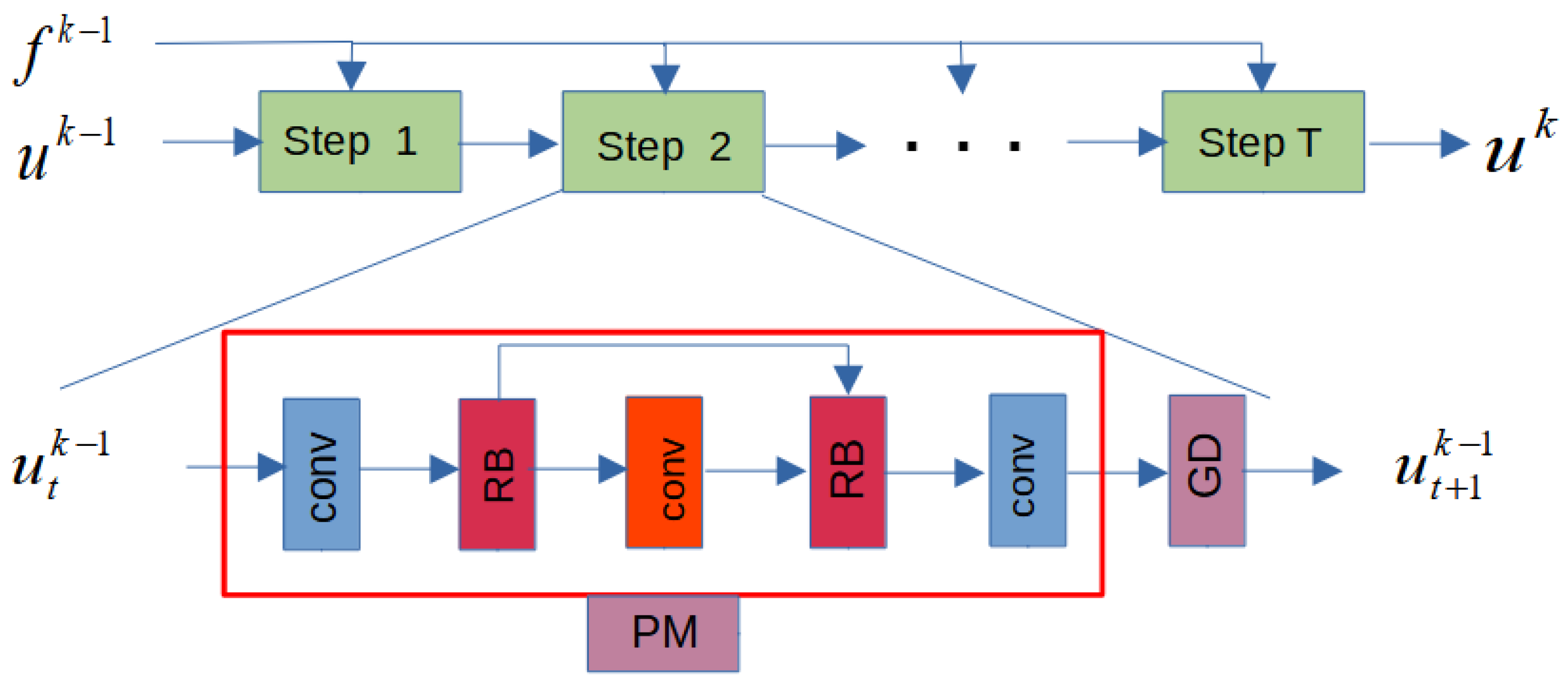
2.2. Reconstruction Subnet

In the reconstruction sub-network (Rec-Net), given the sampling mask S, we solve the optimization problem of the lower layer. The problem is converted to Equation (7)

$$\begin{array}{cc}\mathrm{(7a)}& \underset{R;u_i}{min}{\displaystyle \sum _{i=1}^N}\left|\right|u_i\left(S\right)-u_i^{*}{\left|\right|}_2^2,i=1,\dots ,N\mathrm{(7b)}& s.t.u_i\left(S\right)=arg\underset{u_i}{min}R\left(u_i\right)SF{u}_i=S{y}_i^{*}.& \end{array}$$

This is a constraint problem, which is very difficult to solve, so solving the unconstrained problem shown in Equation (8) is the solution to most of these problems. However, Equation (8) usually requires $\lambda$ to increase during the calculation process to ensure that the constraint approximation holds. However, this destabilizes the data format.

$$u_i\left(S\right)=arg\underset{u_i}{min}R\left(u\right)+\frac{1}{2}\lambda \left|\right|SF{u}_i-S{y}_i^{*}{\left|\right|}_2^2.$$

(8)

In this paper, we introduce a method based on Bregman iterative regularization to find the solution to the constraint problem represented by Equation (7b) by solving a series of continuous unconstrained problems, so as to realize the reconstruction of compressed sensing MRI.

$$\begin{array}{cc}\hfill u^k\left(S\right)=& arg\underset{u}{min}{D}_R^{p^{k-1}}(u,u^{k-1})+\hfill \\ \hfill & \frac{1}{2}\lambda \left|\right|SFu-S{y}^{*}{\left|\right|}_2^2\hfill \\ \hfill p^k=& p^{k-1}-F^{-1}{S}^{-1}(SF{u}^k-S{y}^{*})\hfill \\ \hfill p^0=& 0.\hfill \end{array}$$

(9)

Compared with the traditional penalty function approach, when applied to specific kinds of functions, the Bregman technique achieves high efficiency when the Bergman iterations converge. Moreover, Bregman iteration has another advantage over other methods in that the $\lambda$ in Equation (9) remains unchanged. Therefore, we can choose a $\lambda$ that minimizes the number of conditions for the sub-problem, so that the iterative optimization method converges quickly.

Below, we give an equivalent form of Equation (9) to facilitate the establishment of a network characterization of the regularization term R.

Theorem 1.

Let $f^k=S{y}^{*}+\frac{1}{\lambda }SF{p}^k$, Equation (9) is equivalent to

$$\begin{array}{cc}\hfill & u^k\left(S\right)=arg\underset{u}{min}R\left(u\right)+\frac{1}{2}\lambda \left|\right|SFu-f^{k-1}{\left|\right|}_2^2\hfill \\ \hfill & f^k=f^{k-1}+S{y}^{*}-SF{u}^k.\hfill \end{array}$$

(10)

Proof. 

Let $f^k=S{y}^{*}+\frac{1}{\lambda }SF{p}^k$. Then, by the definition of Bregman distance, we have

$$\begin{array}{cc}\hfill u^k\left(S\right)=& arg\underset{u}{min}{D}_R^{p^{k-1}}(u,u^{k-1})+\frac{1}{2}\lambda \left|\right|SFu-S{y}^{*}{\left|\right|}_2^2\hfill \\ \hfill =& arg\underset{u}{min}R\left(u\right)-〈p^{k-1},u〉\hfill \\ \hfill & +\frac{1}{2}\lambda \left|\right|SFu-S{y}^{*}{\left|\right|}_2^2+C_1\hfill \\ \hfill =& arg\underset{u}{min}R\left(u\right)-〈\lambda F^{-1}{S}^{-1}(f^{k-1}-S{y}^{*}),u〉\hfill \\ \hfill & +\frac{1}{2}\lambda \left|\right|SFu-S{y}^{*}{\left|\right|}_2^2+C_2\hfill \\ \hfill =& arg\underset{u}{min}R\left(u\right)+\frac{1}{2}\lambda \left|\right|SFu-(S{y}^{*}+f^{k-1}-S{y}^{*}){\left|\right|}_2^2\hfill \\ \hfill & +C_3\hfill \\ \hfill =& arg\underset{u}{min}R\left(u\right)+\frac{1}{2}\lambda \left|\right|SFu-f^{k-1}{\left|\right|}_2^2+C_3.\hfill \end{array}$$

(11)

□

Using Theorem 1, we solve the constrained problem represented by Equation (7) by solving a series of unconstrained problems as shown in Equation (10). Intuitively speaking, this brings back the residual of each optimized data item for the next optimization, so that the data item approaches 0 after a series of optimizations and satisfies the constraints. The following theorem proves that the iterative solution $u^k$ to the unconstrained problem shown in Equation (10) is the solution to the original constrained problem represented by Equation (7).

Theorem 2.

Assume that after K stages, $SF{u}^K=S{y}^{*}$ is satisfied. Then, $u^{*}$ is a solution of the original constraint problem represented by Equation (7).

Proof. 

After setting K stages, let $u^K$ and $f^{K-1}$ satisfy $SF{u}^K=S{y}^{*}$ and

$$u^K\left(S\right)=arg\underset{u}{min}R\left(u\right)+\frac{1}{2}\lambda \left|\right|SFu-f^{K-1}{\left|\right|}_2^2.$$

(12)

Let $\widehat{u}$ be a true solution to Equation (7), then $SF{u}^K=S{y}^{*}=SF\widehat{u}$, which implies that

$$\left|\right|SF{u}^K-f^{K-1}{\left|\right|}_2^2=\left|\right|SF\widehat{u}-f^{K-1}{\left|\right|}_2^2.$$

(13)

Because $u^K$ satisfies Equation (12), we have

$$R\left(u^K\right)+\frac{\lambda }{2}\left|\right|SF{u}^K-f^{K-1}{\left|\right|}_2^2\le R\left(\widehat{u}\right)+\frac{\lambda }{2}\left|\right|SF\widehat{u}-f^{K-1}{\left|\right|}_2^2,$$

(14)

then

$$R\left(u^K\right)\le R\left(\widehat{u}\right).$$

(15)

Because $\widehat{u}$ satisfies the original optimization problem represented by Equation (7), this shows that the solution $u^K$ obtained by Equation (10) is indeed the solution to the original constraint problem represented by Equation (7). □

In a subsequent experimental Section 3.3, we will show that the conditions of Theorem 2 are true. By comparing the distances of the constraint terms with learned and radial masks on Brain and Knee datasets, it can be seen that our reconstruction results satisfy the constraints. For fixed stage k, the classical unconstrained optimization problem shown in Equation (10) can be solved by the Gradient-Proximal algorithm. Then, it is effectively solved by iterating over the following two update steps,

$$\begin{array}{ll}\mathrm{(16a)}& r^{k,t}=u^{k,t}-{\rho }_t\left(F^{-1}(SF{u}^{k,t}-f^{k-1})\right)\mathrm{(16b)}& u^{k,t+1}=Pro{x}_R\left(r^{k,t}\right)where\hfill & \\ Pro{x}_R\left(r^{k,t}\right)=arg\underset{u}{min}R\left(u\right)+\frac{\lambda }{2}\left|\right|u-r^{k,t}{\left|\right|}_2^2\hfill & \\ {\rho }_t^k\ge 0,t=1,\dots ,T.\hfill & \end{array}$$

Equations (16b) and (16a) are often referred to as the proximal mapping step (PM) and gradient descent step (GD), respectively. Finding an effective way to solve the PM step is crucial for CS problems. Since the $Pro{x}_R$ operator is similar to denoising, a lot of work [22,29] has been done to learn this operator using a denoising network to obtain adaptive regularized R. Similarly, in this paper, the traditional Equation (16b) formula is converted to the form of a deep network to build a deep unfolding network (Equation (17)). In this way, the lower-level optimization problem is transformed into a phase reconstruction problem, and each stage adds the residual of the previous stage data items to the next stage of training. For each PM step, instead of using a ready-made denoising network, we propose a lightweight and effective network module PM to complete, which can be expressed as:

$$\begin{array}{cc}\hfill & u^{k,t+1}=PM{M}_{\theta }\left(r^{k,t}\right)\hfill \\ \hfill & Where\hfill \\ \hfill & PM{M}_{\theta }\left(r^{k,t}\right)=r^{k,t}+{\beta }_t\left(H_{rec}{H}_{RB2}\left(H\left(H_{RB}{H}_{ext}{r}^{k,t}\right)\right)\right),\hfill \end{array}$$

(17)

where $PM$ consists of two convolutional blocks $H_{RB}$ and three convolutional layers, $H_{ext}$, $H_{rec}$, respectively, for extracting image features and reconstruction and connecting with the long residual of the input, and $\theta$ are learnable network parameters.

Figure 2 and Figure 3 show the stage unfolding to rebuild the sub-network, which consists of K stages, each corresponding to an optimization problem in the Bregman iteration. Each stage has T steps, each consisting of a proximal mapping module ($PM$) and a gradient descent module ($GD$), which correspond to the two update steps Equations (16b) and (16a) described above.

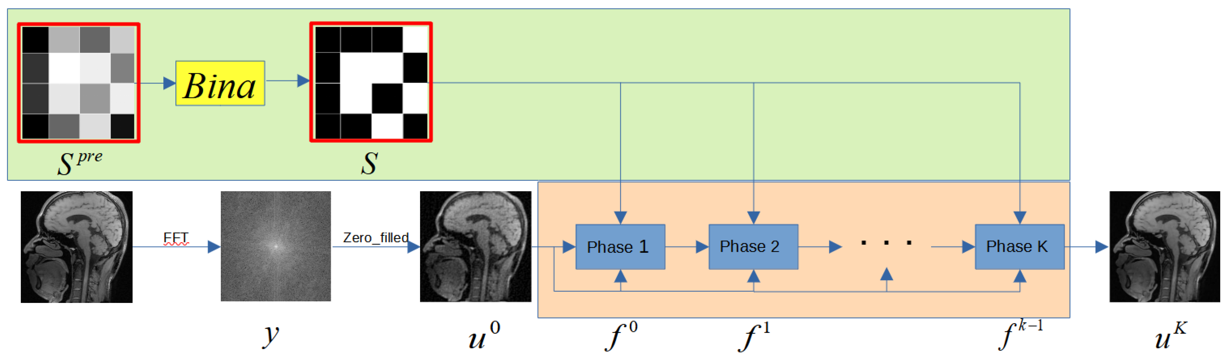
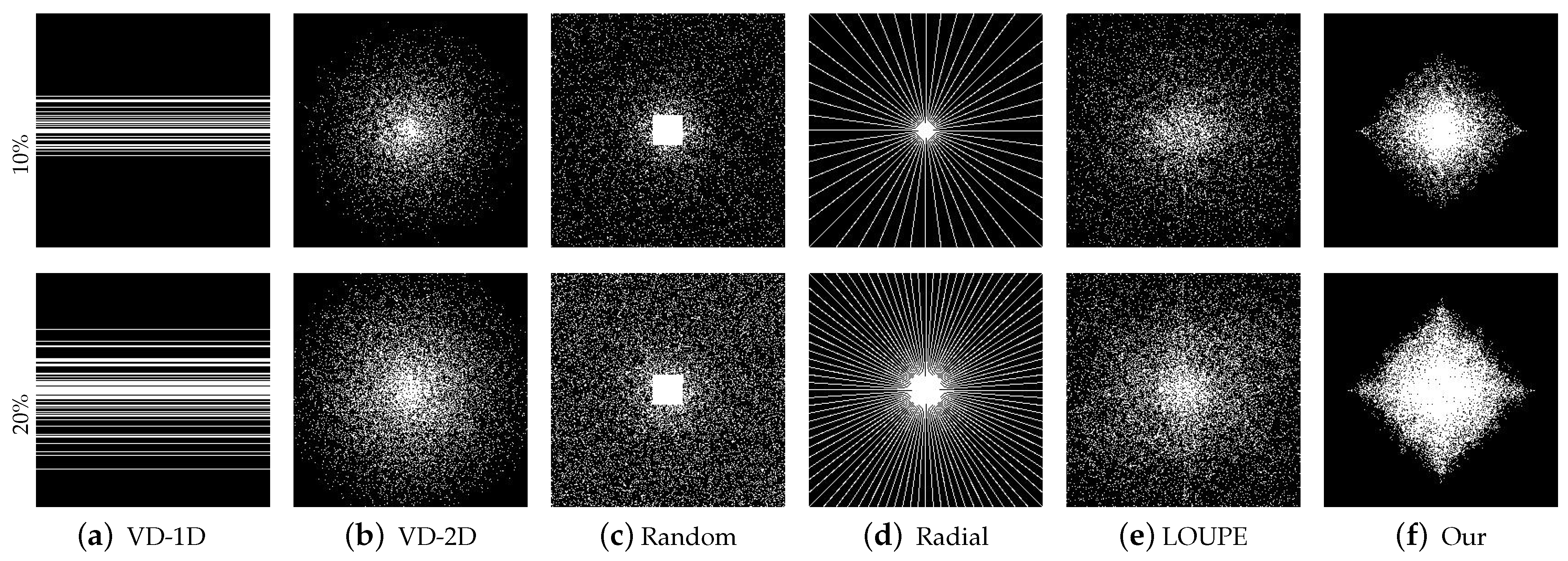
2.3. Sampling Subnet

In the sampling subnet (Samp-Net), given the sampling mask S, the solution $u_i^K\left(S\right)$ of the lower optimization problem is obtained, and the sampling mask S in the upper optimization problem is updated by the formula given in Equation (18). By adding penalty terms to the gradient, the sampling mask is encouraged to achieve the desired sparsity. The optimization problem is then transformed into

$$\begin{array}{cc}\mathrm{(18a)}& \underset{S,u_i}{min}L={\displaystyle \sum _{i=1}^N}\left|\right|u_i^K(S;\theta )-u_i^{*}{\left|\right|}_2^2,i=1,\dots ,N\mathrm{(18b)}& s.t.u_i^k(S;\theta )=PM{M}_{\theta }^k\left(GD{M}_{\theta }^k\left(u_i^{k-1}\right)\right)k=1,\dots ,K\hfill & \\ S\in \left\{0,1\right\}\hfill & \\ {\left|\right|S\left|\right|}_0=Sp\_exp.\hfill & \end{array}$$

Through the back-propagation of the network, the gradient of L to S in the lower model is calculated, such as formula given in Equation (19), where $S\in \left\{0,1\right\}$.

$${\nabla }_{s}L=(2(u^K\left(S\right)-u^{*})\nabla u^K\left(S\right)).$$

(19)

We introduce a learnable sampling pattern $S^{Pre}$, each value $S_{i,j}^{Pre}\in \left[-1,1\right]$ represents the weight of this point, and use the strategy of accumulating gradients to learn the weight of each point in the sampling pattern. The higher the weight learned, the more important this point is, and the data of this point should be sampled.

$$\begin{array}{}\mathrm{(20a)}& S^{Pre}=S^{Pre}-\rho \nabla Bina\left(S^{Pre}\right)\left({\nabla }_{s}L\right)\mathrm{(20b)}& whereBina\left(x\right)=\left\{\begin{array}{c}1,x\ge 0\hfill \\ 0,x<0.\hfill \end{array}\right.\end{array}$$

In back-propagation, we update the weights on learnable sampling mask $S^{Pre}$ by gradient descent (Equation (20a)).

Because $Bina\left(x\right)$ is not differentiable, we refer to the gradient update method of the binary neural network [40,41,42], replace the derivative of $Bina\left(x\right)$ with the derivative of $tanh\left(gx\right)$, and perform the reverse derivation, such as shown in Equation (21).

$$S^{Pre}=S^{Pre}-\rho ·g(1-tanh(g·S^{Pre})\left({\nabla }_{s}L\right).$$

(21)

As the training progresses, g slowly becomes larger, the function becomes closer and closer to the binary function, and at the same time, pays more attention to the derivative of the point around 0. Thereby, the dynamic gradient strategy can achieve effective training and improve network performance. In order to ensure that the learned sampling mask reaches the desired sampling ratio, we encourage the sampling mask to achieve the desired sampling rate by imposing a penalty term on the gradient. Since the true weight of the sampling mask is not required, only the relative weight size needs to be obtained, and a penalty factor is directly applied to the gradient of the back-propagation, such as shown in Equation (22), where $\alpha$ is the penalty factor.

$$S^{Pre}=S^{Pre}-\rho ·g(1-tanh(g·S^{Pre})({\nabla }_{s}L+\alpha ).$$

(22)

Regarding the selection of $\alpha$, we chose a series with a small initial value that can be dynamically adjusted according to the sampling rate for sparse penalty, such that when ${\left|\right|S\left|\right|}_0-Sp\_exp>\epsilon ,{\alpha }_{k+1}=c·{\alpha }_k,c>1$ and when ${\left|\right|S\left|\right|}_0-Sp\_exp<-\epsilon ,{\alpha }_{k+1}=c·{\alpha }_k,c<1$. In simple terms, when the sampling ratio exceeded the desired sparsity, the penalty should be increased, and vice versa, and the number of points $S_{i,j}^{Pre}$ should be guaranteed in the end to be equivalent to the desired number of samples.

In forward propagation, Equation (23) is used to binarize these weights, and then the activated mask is fed into the reconstructed subnet together with the original data for learning.

$$\begin{array}{cc}\hfill & S=Bina\left(S^{Pre}\right).\hfill \end{array}$$

(23)

The gradient in the equation Equation (22) ${\nabla }_{s}L$ is obtained by the back-propagation of the neural network, and the latter part of the gradient $\alpha$ is obtained by directly applying the sparse penalty term, and is transmitted back to the sampling sub-network for update, while $tanh\left(gx\right)$ gradually approximates the binarization function, reasonably updates all parameters, effectively retains the gradient information, and improves the network performance. In addition, the output of the sampling subnet meets the two constraints of sparsity and binarization, which reduces the learning difficulty of reconstructing the subnet.

2.4. Initialization and Parameters

Given the training dataset and full-resolution image ${\left(u_i^{*}\right)}_{i=1}^N$, the corresponding analog measurement $y_i^{*}=F{u}_i^{*}$ is obtained, and the sampling sub-network first uses a learnable sampling mask S. The initial value of S is Gaussian white noise with a mean of 0 and an variance of 0.1. Then, with initialization $u_i^0=F^{-1}S{y}_i^{*}$ as input, the reconstruction subnet outputs the recovery results, aiming to reduce the difference between $u_i^{*}$ and $u_i^K$. $\theta$ in Equation (17) is a learnable network parameter.

3. Experiment

Our model, built using PyTorch, is implemented on an NVIDIA V100 GPU. Using Adam optimization to optimize the model, the learning rate is 0.001. We use a 6-layer network module to correspond to the 6 Bregman sub-problems and set the batch size to 8. The default value for each stage step is 1. As is common in previous work, we use two widely used benchmark datasets, Brain and Fast-MRI [43], which contain 100 brain and 90 volumes of knee MR images for training and 50 brain and 10 rolls of knee MR images for testing, respectively. The results of recovery were evaluated using peak signal-to-noise ratio (PSNR) and the structural similarity index (SSIM [44]).

3.1. Comparison with Classical Masking under Multiple Reconstruction Methods

To verify the effectiveness of our proposed sampling mask optimization scheme, the learnable masks are compared with five masks under three classical reconstruction methods, including four classical fixed masks and one probability-based learnable mask.

In terms of classical fixed masks, we employed widely used approaches from the literature in four categories: skipped-line Cartesian mask (denoted as $VD-1D$), radial mask [5], random uniform mask [4], and Variable Density $-2D$ (denoted as $VD-2D$) [5] mask. The first is a $1D$ sub-sampling mask and the last three are $2D$ masks. In terms of learnable masks, we used LOUPE [34] for comparison.

For the reconstruction method, a traditional model-based approach, BM3D-MRI [32], a widely used deep learning model, U-Net [17], and our reconstruction sub-network are considered for fair comparison.

Figure 4 shows a visual comparison between the classical mask and our trained optimized sub-sampling ratio for ${\left|\right|S\left|\right|}_0=10\%$ and ${\left|\right|S\left|\right|}_0=20\%$. It can be seen that the learned $2D$ mask exhibits a strong preference for lower frequencies and a denser sampling pattern closer to the origin of K-space, which is also in line with prior knowledge, i.e., the lower frequency part has greater energy.

Table 1. PSNR comparison with Classical Masking under Multiple Reconstruction Methods and a CS Ratio of 5%.

Brain
Method	VD-2D	Random	Radial	LOUPE	Proposed
BM3D-MRI	32.12	32.98	31.84	34.62	34.84
U-Net	32.41	32.91	31.21	34.78	35.34
OUR	32.49	32.37	31.77	34.66	35.62

lists the specific PSNR values when the CS ratio is set to 5%. As can readily be observed, the highest PSNR results can be obtained through the use of the proposed Samp-Net, which benefits from the efficient probabilistic under-sampling scheme. Taking the $5\%$ ratio of reconstructing the sub-network as an example, our Samp-Net achieves a significant 0.98 dB PSNR gain over the probability-based learnable mask LOUPE. This is because our learnable mask learns the point with the greatest weight of the fixed sample rate, and, as can also be seen from Figure 4, our learnable mask has a clearer structure and better represents the data structure of the dataset. It is also worth noting that U-Net still performs worse than our unfolding net when equipped with our Samp-Net, which indicates that deep unfolding networks incorporating prior knowledge are more suitable for promoting exploration and efficient training of our Samp-Net than classical data-driven reconstruction models. Figure 5 further shows a comparison of visual reconstructions under the reconstructed subnet when the CS ratio is set to 10%. From the comparison images, it is intuitive to see that the sampling mask learned using our proposed approach is able to consistently restore more detail and sharper edges than the other masks in the comparison.

In addition, Figure 6 compares the differences in the anatomical optimization of the knee and brain joints of our model. We observed that for MR images of the knee, due to the unique asymmetrical features of knee anatomy, give more importance to the lateral frequency direction, with obvious tissue contrasts. Conversely, the masks learned on the Brain dataset appear to be more balanced in all frequency directions. Such data comparison results show the importance of learnable masks, and it is necessary to customize sampling masks of different structures for data with different structures. It is worth noting that the masks learned on the Brain and Knee datasets at $10\%$ show high intermediate density and low peripheral density. At $20\%$, the Knee mask maintains this feature, but the Brain mask has a high density within its data structure, which may indicate that the sampling ratio of $20\%$ is good enough to restore good results for the Brain dataset but not for the Knee dataset. The experimental results given in

Table 2. PSNR and SSIM comparison of our proposed model with state-of-the-art methods.

Dataset	Method	Mask	CS Ratio
			5%	10%	20%
Brain	Zero _ Filled	Radial	25.31/0.5824	27.02/0.6085	29.12/0.6717
	U-Net		32.13/0.8433	35.21/0.8874	38.35/0.9328
	Admm-Net		31.48/0.8371	34.92/0.9052	37.72/0.9343
	Ista-Net		31.72/0.8453	34.66/0.8692	37.49/0.9404
	LOUPE	1d	32.17/0.8233	35.49/0.9140	36.62/0.9136
		2d	35.66/0.9121	38.16/0.9259	39.21/0.9473
	PUERT	1d	32.33/0.8677	35.82/0.9142	37.17/0.9227
		2d	35.48/0.9027	38.23/0.9410	39.74/0.9590
	Proposed	1d	32.14/0.8414	35.61/0.9167	37.22/0.9214
		2d	36.12/0.9245	38.56/0.9345	39.41/0.9526
Knee	Zero _ Filled	Radial	24.93/0.5930	27.56/0.6227	28.71/0.6564
	U-Net		29.17/0.6618	32.54/0.6866	35.66/0.7930
	Admm-Net		29.05/0.6927	32.06/0.7280	35.24/0.8057
	Ista-Net		29.41/0.6714	31.97/0.7043	35.08/0.7794
	LOUPE	1d	30.37/0.6991	31.93/0.7178	33.85/0.7428
		2d	31.46/0.7316	34.14/0.7671	36.41/0.8590
	PUERT	1d	30.71/0.6824	32.57/0.7143	34.23/0.7411
		2d	31.76/0.7230	34.02/0.7573	36.24/0.8568
	Proposed	1d	30.47/0.6726	33.61/0.7268	34.28/0.7467
		2d	32.57/0.7557	34.41/0.7829	36.36/0.8624

also illustrate this.

Figure 7 compares the probability-based mask with our mask on the Brain dataset. The sampling ratio is $5\%$, and the blue curve is the progress curve of PSNR results when equipping our mask, while the red curve is the progress curve of PSNR results when equipping LOUPE. In order to make a fair comparison, the reconstruction algorithm is U-NET for both. It can be seen that our mask can not only achieve convergence faster, but also the final PSNR result is higher than with LOUPE. These results emphasize that good masks can help reconstruction algorithms to achieve better results. It is worth noting that our mask also has a better structure than LOUPE in the zero-filled state, which can speed up the inference of the model.

3.2. Comparison with State-of-the-Art Methods

We compare the proposed reconstruction model with five representative state-of-the-art methods, namely U-Net [17], ADMM-Net [29], ISTA-Net [15], PUERT [22], and LOUPE [34]. The first three methods are reconstructed networks trained under a certain fixed sampling mask, while the latter two methods jointly optimize the learnable sampling mask and reconstruction network parameters. When performing comparative experiments, we used radial masks on the Brain and FastMRI datasets for tasks trained under fixed masks. Three learnable sampling masks enable both $1-D$ and $2-D$ sub-sampling optimization. Table 2 summarize the average PSNR/SSIM performance reconstruction at three CS ratios by various methods on the two datasets. It can be observed from the table that methods that use learnable sampling patterns generally produce higher PSNR than those with fixed masks, which confirms the superiority of the learned sampling mode.

Specifically, compared with the probability-based sampling mode optimization scheme employed by LOUPE and PUERT, it can be seen that at a sampling ratio of $5\%$, the PSNR and SSIM of our model are significantly improved on both the Fast-MRI and Brain datasets. This is due to the fact that the data structure learned by our sampling mask is more pronounced at low sampling rates. On the Brain dataset, the gap between the proposed model and the results produced by PUERT $-2D$ and LOUPE $-2D$ narrows as the sampling ratio increases, which also shows that as previously mentioned, a $20\%$ sampling ratio can restore good results. On the Knee dataset, under three different sampling ratios, the proposed model performs slightly better than PUERT and LOUPE. In particular, at a sampling ratio of $5\%$, the PSNR obtained is significantly increased by 0.77 compared with the PUERT results. This is because, with the large dataset, the sampling ratio is $20\%$ is still not enough for the Knee dataset. Under these circumstances, prior knowledge of the data structure is particularly important, while the masks we learn can help the reconstruction task. It can be observed from Table 2 that the use of neural networks enable five representative state-of-the-art methods to achieve real-time reconstruction speeds. As is shown in Figure 8, with a CS ratio of $10\%$, the proposed model produces more reliable and clearer visual reconstructions than the other models in the comparison. In conclusion, the two experiments using two widely used MRI datasets indicate that the proposed model is superior to state-of-the-art methods in both quantitative indicators and visual quality.

When we explore the influence of constraints on two sampling masks (radial mask [blue] and learnable [red] mask (Figure 9)), it can be seen that in the two datasets with these two sampling masks, as the training progresses, the constraint items tend to 0, which satisfies the condition of Theorem 2. A solution obtained by training is then a solution $u^K$ to the constraint problem represented by Equation (7b). Of the two masks, the learnable mask can better help the lower-level optimization problem meet the constraints and improve the restoration quality.

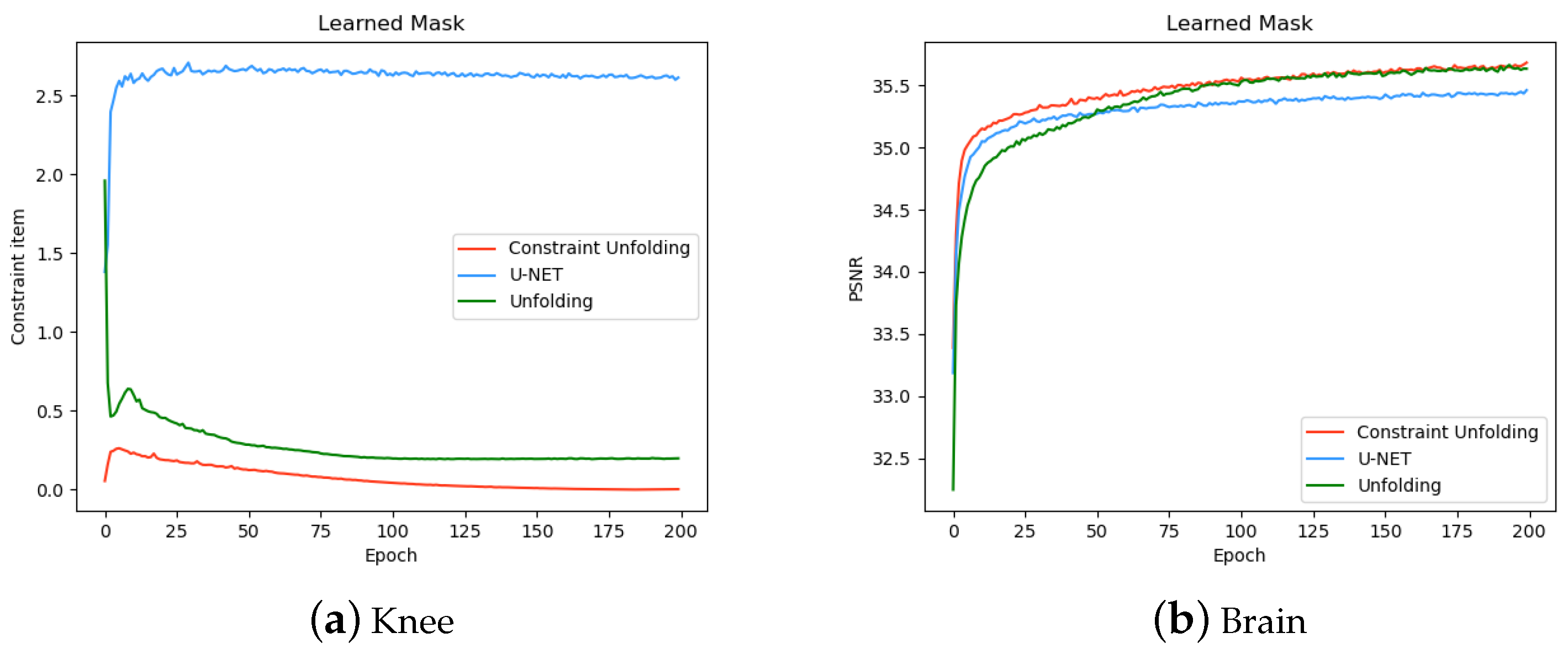
3.3. Effect of Data Constraints

In Theorem 2, it is shown that if after K stages, $u^K$ satisfies $SF{u}^K=S{y}^{*}$, then a solution $u^K$ obtained by Equation (10) is a solution of the original constraint problem represented by Equation (7b). We illustrate this with numerical experiments on the Brain and Knee datasets.

We also explore the influence of a pure U-NET network, a traditional deep unfolding network, and our constrained deep unfolding network under constraints on the Brain and Knee Datasets. A learnable mask is used. As can be seen from the results shown in Figure 10a (blue is U-NET [17], red is our reconstruction subnet, green is the traditional deep unfolded network [22]), the reconstruction results obtained by U-NET do not make good use of the existing sampling information, and there is a gap between reconstruction results and the real frequency domain data, while our constrained deep unfolding network satisfies the constraint conditions better than the traditional deep unfolding network, and can better use the prior knowledge brought by the sampling mask. Figure 10b compares the gap between the three in reconstruction quality, and both deep unfolded networks achieve higher indicators than the U-NET method. Our model imposes regularity on the results of the reconstruction, so as to better meet the constraints and make the reconstructed image more realistic.

4. Conclusions

In this paper, we simultaneously and effectively deal with two problems in CS-MRI, the selection of sampling masks and the design of reconstruction algorithms, by combining sub-sampling learning with reconstruction network training. The sampling subnet learns the weight of each sampling point and obtains the sampling mask under each sampling ratio according to the size of the weight. Using the Bregman algorithm of the data item constraint optimization problem, a new phase deep unfolding reconstruction network is proposed, which uses a series of unconstrained iterative solutions to solve the constraint problem. When tested on two widely used MRI datasets, the experimental results verify that our model produces good results in terms of both quantitative indicators and visual quality. It also produces significant results at challengingly low sampling ratios.

References

1. Lustig, M.; Donoho, D.L.; Santos, J.M.; Pauly, J.M. Compressed sensing MRI. IEEE Signal Process. Mag. 2008, 25, 72–82. [Google Scholar] [CrossRef]
2. Lustig, M.; Donoho, D.; Pauly, J.M. Sparse MRI: The application of compressed sensing for rapid MR imaging. Magn. Reson. Med. 2007, 58, 1182–1195. [Google Scholar] [CrossRef] [PubMed]
3. Haldar, J.P.; Hernando, D.; Liang, Z.-P. Compressed-Sensing MRI With Random Encoding. IEEE Trans. Med Imaging 2010, 30, 893–903. [Google Scholar] [CrossRef]
4. Gamper, U.; Boesiger, P.; K ó zerke, S. Compressed sensing in dynamic MRI. Magn. Reson. Med. 2008, 59, 365–373. [Google Scholar] [CrossRef]
5. Letourneau, M.; Sharp, J.W.; Wang, Z.; Arce, G.R. Variable density compressed image sampling. IEee Trans. Image Process. 2009, 19, 264–270. [Google Scholar]
6. Yiasemis, G.; Zhang, C.; Sánchez, C.I.; Fuller, C.D.; Teuwen, J. Deep MRI reconstruction with radial subsampling. Med. Imaging 2022 Phys. Med. Imaging 2022. [Google Scholar] [CrossRef]
7. Lustig, M.; Pauly, J.M. SPIRiT: Iterative self-consistent parallel imaging reconstruction from arbitrary k-space. Magn. Reson. Med. 2010, 64, 457–471. [Google Scholar] [CrossRef]
8. Ehrhardt, M.; Betcke, M.M. Multi-Contrast MRI Reconstruction with Structure-Guided Total Variation. Siam J. Imaging Sci. 2016, 9, 1084–1106. [Google Scholar] [CrossRef]
9. Block, K.T.; Uecker, M.; Frahm, J. Undersampled radial MRI with multiple coils. Iterative image reconstruction using a total variation constraint. Magn. Reson. Med. 2007, 57, 1086–1098. [Google Scholar] [CrossRef]
10. Trzasko, J.; Manduca, A. Highly Undersampled Magnetic Resonance Image Reconstruction via Homotopic l0-Minimization. IEEE Trans. Med. Imaging 2009, 28, 106–121. [Google Scholar] [CrossRef]
11. Qu, X.; Guo, D.; Ning, B.; Hou, Y.; Lin, Y.; Cai, S.; Chen, Z. Undersampled MRI reconstruction with patch-based directional wavelets. Magn. Reson. Imaging 2012, 30, 964–977. [Google Scholar] [CrossRef]
12. Yang, J.; Zhang, Y.; Yin, W. A fast alternating direction method for TVL1-L2 signal reconstruction from partial fourier data. IEEE J. Sel. Top. Signal Process. 2010, 4, 288–297. [Google Scholar] [CrossRef]
13. Osher, S.; Burger, M.; Goldfarb, D.; Xu, J.; Yin, W. An Iterative Regularization Method for Total Variation-Based Image Restoration. Multiscale Model. Simul. 2005, 4, 460–489. [Google Scholar] [CrossRef]
14. Zhang, K.; Gool, L.V.; Timofte, R. Deep Unfolding Network for Image Super-Resolution. In Proceedings of the 2020 IEEE/CVF Conference on Computer Vision and Pattern Recognition (CVPR), Seattle, WA, USA, 13–19 June 2020. [Google Scholar]
15. Zhang, J.; Ghanem, B. ISTA-Net: Interpretable optimization-inspired deep network for image compressive sensing. In Proceedings of the IEEE Conference on Computer Vision and Pattern Recognition (CVPR), Salt Lake City, UT, USA, 18–23 June 2018. [Google Scholar]
16. Qin, C.; Schlemper, J.; Caballero, J.; Price, A.N.; Hajnal, J.V.; Rueckert, D. Convolutional Recurrent Neural Networks for Dynamic MR Image Reconstruction. IEEE Trans. Med Imaging 2018, 38, 280–290. [Google Scholar] [CrossRef]
17. Ronneberger, O.; Fischer, P.; Brox, T. “U-net: Convolutional networks for biomedical image segmentation. In Proceedings of the International Conference on Medical Image Computing and Computer-Assisted Intervention (MICCAI), Munich, Germany, 5–9 October 2015. [Google Scholar]
18. Goodfellow, I.; Pouget-Abadie, J.; Mirza, M.; Xu, B.; Warde-Farley, D.; Ozair, S.; Courville, A.; Bengio, Y. Generative adversarial nets. In Proceedings of the Advances in Neural Information Processing Systems (NeurIPS), Montreal, QC, Canada, 8–13 December 2014. [Google Scholar]
19. Ledig, C.; Theis, L.; Huszár, F.; Caballero, J.; Cunningham, A.; Acosta, A.; Aitken, A.P.; Tejani, A.; Totz, J.; Wang, Z.; et al. Photo-Realistic Single Image Super-Resolution Using a Generative Adversarial Network. In Proceedings of the 2017 IEEE Conference on Computer Vision and Pattern Recognition (CVPR), Honolulu, HI, USA, 21–26 July 2017. [Google Scholar]
20. Martinez, B.; Yang, J.; Bulat, A.; Tzimiropoulos, G. Training binary neural networks with real-to-binary convolutions. arXiv 2019, arXiv:2003.11535. [Google Scholar]
21. Matthieu, C.; Itay, H.; Daniel, S.; Ran, E.; Yoshua, B. Bi-narized Neural Networks: Training Deep Neural Networks with Weights and ActivationsConstrained to +1 or −1. arXiv 2016, arXiv:1602.02830. [Google Scholar]
22. Xie, J.; Zhang, J.; Zhang, Y.; Ji, X. PUERT: Probabilistic Under-Sampling and Explicable Reconstruction Network for CS-MRI. IEEE J. Sel. Top. Signal Process. 2022, 16, 737–749. [Google Scholar] [CrossRef]
23. Benning, M.; Gladden, L.; Holland, D.; Schönlieb, C.-B.; Valkonen, T. Phase reconstruction from velocity-encoded MRI measurements—A survey of sparsity-promoting variational approaches. J. Magn. Reson. 2014, 238, 26–43. [Google Scholar] [CrossRef]
24. Zhao, N.; Wei, Q.; Basarab, A.; Dobigeon, N.; Kouamé, D.; Tourneret, J.-Y. Fast Single Image Super-Resolution Using a New Analytical Solution for l2 − l2 Problems. IEEE Trans. Image Process. 2016, 25, 3683–3697. [Google Scholar] [CrossRef]
25. Nikam, R.D.; Lee, J.; Choi, W.; Kim, D.; Hwang, H. On-Chip Integrated Atomically Thin 2D Material Heater as a Training Accelerator for an Electrochemical Random-Access Memory Synapse for Neuromorphic Computing Application. ACS Nano 2022, 16, 12214–12225. [Google Scholar] [CrossRef]
26. Nikam, R.D.; Kwak, M.; Hwang, H. All-Solid-State Oxygen Ion Electrochemical Random-Access Memory for Neuromorphic Computing. Adv. Electron. Mater. 2021, 7, 2100142. [Google Scholar] [CrossRef]
27. Aggarwal, H.K.; Jacob, M. J-MoDL: Joint Model-Based Deep Learning for Optimized Sampling and Reconstruction. IEEE J. Sel. Top. Signal Process. 2020, 14, 1151–1162. [Google Scholar] [CrossRef] [PubMed]
28. Wang, S.; Su, Z.; Ying, L.; Peng, X.; Zhu, S.; Liang, F.; Feng, D.; Liang, D. Accelerating magnetic resonance imaging via deep learning. In Proceedings of the 2016 IEEE 13th International Symposium on Biomedical Imaging (ISBI), Prague, Czech Republic, 13–16 April 2016. [Google Scholar]
29. Yang, Y.; Sun, J.; Li, H.; Xu, Z. Deep ADMM-Net for compressive sensing MRI. In Proceedings of the Advances in Neural Information Processing Systems (NeurIPS), Barcelona, Spain, 5–10 December 2016. [Google Scholar]
30. Yang, G.; Yu, S.; Dong, H.; Slabaugh, G.; Dragotti, P.L.; Ye, X.; Liu, F.; Arridge, S.; Keegan, J.; Guo, Y.; et al. DAGAN: Deep De-Aliasing Generative Adversarial Networks for Fast Compressed Sensing MRI Reconstruction. IEEE Trans. Med. Imaging 2018, 37, 1310–1321. [Google Scholar] [CrossRef]
31. Jun, Y.; Shin, H.; Eo, T.; Hwang, D. Joint Deep Model-based MR Image and Coil Sensitivity Reconstruction Network (Joint-ICNet) for Fast MRI. In Proceedings of the 2021 IEEE/CVF Conference on Computer Vision and Pattern Recognition, Nashville, TN, USA, 20–25 June 2021. [Google Scholar]
32. Eksioglu, E.M. Decoupled Algorithm for MRI Reconstruction Using Nonlocal Block Matching Model: BM3D-MRI. J. Math. Imaging Vis. 2016, 56, 430–440. [Google Scholar] [CrossRef]
33. Chen, S.; Luo, C.; Deng, B.; Qin, Y.; Wang, H.; Zhuang, Z. BM3D vector approximate message passing for radar coded-aperture imaging. In Proceedings of the 2017 Progress in Electromagnetics Research Symposium—Fall (PIERS—FALL), Singapore, 19–22 November 2017. [Google Scholar]
34. Bahadir, C.D.; Wang, A.Q.; Dalca, A.V.; Sabuncu, M.R. Deep-Learning-Based Optimization of the Under-Sampling Pattern in MRI. IEEE Trans. Comput. Imaging 2020, 6, 1139–1152. [Google Scholar] [CrossRef]
35. Lee, D.H.; Hong, C.P.; Lee, M.W.; Kim, H.J.; Jung, J.H.; Shin, W.H.; Kang, J.; Kang, S.; Han, B.S. Sparse sampling MR image reconstruction using bregman iteration: A feasibility study at low tesla MRI system. In Proceedings of the 2011 IEEE Nuclear Science Symposium Conference Record, Valencia, Spain, 23–29 October 2011. [Google Scholar]
36. Zibetti, M.V.W.; Herman, G.T.; Regatte, R.R. Fast data-driven learning of parallel MRI sampling patterns for large scale problems. Sci. Rep. 2021, 11, 19312. [Google Scholar] [CrossRef]
37. Choi, J.; Kim, H. Implementation of time-efficient adaptive sampling function design for improved undersampled MRI reconstruction. J. Magn. Reson. 2016, 273, 47–55. [Google Scholar] [CrossRef]
38. Gözcü, B.; Mahabadi, R.K.; Li, Y.H.; Ilıcak, E.; Cukur, T.; Scarlett, J.; Cevher, V. Learning-based compressive MRI. IEEE Trans. Med. Imaging 2018, 37, 1394–1406. [Google Scholar]
39. Sherry, F.; Benning, M.; De los Reyes, J.C.; Graves, M.J.; Maierhofer, G.; Williams, G.; Schönlieb, C.; Ehrhardt, M.J. Learning the sampling pattern for MRI. IEEE Trans. Med. Imaging 2020, 39, 4310–4321. [Google Scholar] [CrossRef]
40. Simons, T.; Lee, D.-J. A Review of Binarized Neural Networks. Electronics 2019, 8, 661. [Google Scholar] [CrossRef]
41. Alizadeh, M.; Fernández-Marqués, J.; Lane, N.D.; Gal, Y. An empirical study of binary neural networks optimisation. In Proceedings of the International Conference on Learning Representations, New Orleans, LA, USA, 6–9 May 2019. [Google Scholar]
42. Lin, X.; Zhao, C.; Pan, W. Towards accurate binary convolutional neural network. In Proceedings of the 31st International Conference on Neural Information Processing Systems, Long Beach, CA, USA, 4–9 December 2017. [Google Scholar]
43. Zbontar, J.; Knoll, F.; Sriram, A.; Murrell, T.; Huang, Z.; Muckley, M.J.; Defazio, A.; Stern, R.; Johnson, P.; Bruno, M.; et al. FastMRI: An open dataset and benchmarks for accelerated MRI. arXiv 2018, arXiv:1811.08839. [Google Scholar]
44. Wang, Z.; Bovik, A.C.; Sheikh, H.R.; Simoncelli, E.P. Image Quality Assessment: From Error Visibility to Structural Similarity. IEEE Trans. Image Process. 2004, 13, 600–612. [Google Scholar] [CrossRef] [PubMed]
Figure 1. Our model consists of two parts, the sampling subnet (green shaded area) and the reconstruction subnet (orange shaded area). The learnable sampling mask is fused with the initial under-sampled image after binary activation and reconstructed image in K stages.
Electronics 12 04657 g001
Figure 2. Each stage contains T steps, each step has a PM and a GD, and at the same time, to add the last updated f k to the GD, we place the GD after the PM to better complete the constraint task. Each PM consists of 2 convolutional blocks H R B and three convolutional layers, H e x t , H r e c , respectively, for extracting image features and reconstruction and connecting with the long residual of the input.
Electronics 12 04657 g002
Figure 3. Each convolutional blocks contains two convolutional layers and two activation layers.
Electronics 12 04657 g003
Figure 4. Visual comparison of different masks on the Brain dataset. The CS ratios are set to 10% and 20%. Our learnable masks have a clearer data structure than other masks, and also satisfy the priors of low frequency density and high frequency sparseness.
Electronics 12 04657 g004
Figure 5. Visual reconstruction comparison of different masks on the Brain dataset with a CS ratio of 10%.The PSNR values of the reconstructed results are also listed. Our proposed model can recover more detail and sharper edges.
Electronics 12 04657 g005
Figure 6. Visual comparison of learned masks on Brain and Knee datasets with CS ratios of 10% and 20%. The masks learned on the Knee dataset appear to give more importance to the lateral frequency direction, with obvious tissue contrasts, while the masks learned on the Brain dataset appear to be more balanced in all frequency directions.
Electronics 12 04657 g006
Figure 7. PSNR comparison of two learnable masks under the U-NET method on the Brain dataset. Our learnable masks can complete reconstruction tasks faster and better, achieve higher PSNR indicators, and have better visual effects than the LOUPE mask under the zero _ filled method.
Electronics 12 04657 g007
Figure 8. Visual reconstruction comparisons with various state-of-the-art methods on the FastMRI [43] dataset with a CS ratio of 10%. Our model can recover more realistic details without producing overly smooth results.
Electronics 12 04657 g008
Figure 9. By comparing the distances of the constraint terms with learned and radial masks on the Brain and Knee datasets, it can be seen that our reconstruction results satisfy the constraints.
Electronics 12 04657 g009
Figure 10. When equipped with learnable masks on the Brain and Knee datasets and under a CS ratio of 5%, a comparison of the constraint term distance and PSNR of the three reconstruction methods shows that our constraint model makes better use of the sampled real data, better meets the constraints, and returns more realistic reconstruction results.
Electronics 12 04657 g010