Article

Dataset Bias Prediction for Few-Shot Image Classification

1
Department of Artificial Intelligence, Ajou University, Suwon 16499, Republic of Korea
2
Department of Software and Computer Engineering, Ajou University, Suwon 16499, Republic of Korea
*
Author to whom correspondence should be addressed.
Electronics 2023, 12(11), 2470; https://doi.org/10.3390/electronics12112470
Submission received: 8 April 2023 / Revised: 17 May 2023 / Accepted: 28 May 2023 / Published: 30 May 2023

Abstract

:
Dataset bias is a significant obstacle that negatively affects image classification performance, especially in few-shot learning, where datasets have limited samples per class. However, few studies have focused on this issue. To address this, we propose a bias prediction network that recovers biases such as color from the extracted features of image data, resulting in performance improvement in few-shot image classification. If the network can easily recover the bias, the extracted features may contain the bias. Therefore, the whole framework is trained to extract features that are difficult for the bias prediction network to recover. We evaluate our method by integrating it with several existing few-shot learning models across multiple benchmark datasets. The results show that the proposed network can improve the performance in different scenarios. The proposed approach effectively reduces the negative effect of the dataset bias, resulting in the performance improvements in few-shot image classification. The proposed bias prediction model is easily compatible with other few-shot learning models, and applicable to various real-world applications where biased samples are prevalent, such as VR/AR systems and computer vision applications.

1. Introduction

Few-shot learning, which trains a model with only a few training samples, is a challenging area of machine learning. Numerous models have been proposed for few-shot learning [1,2,3,4,5,6,7,8,9,10,11,12,13,14]. Generally, in few-shot learning, it is essential to quickly adapt to new classes because there are a large number of classes to classify. To fulfill this requirement, many recent works have utilized meta-learning as an effective technique for training and classifying samples in few-shot learning [4,5,6,11,15].
Few-shot learning is an important technique for machine learning systems based on VR (Virtual Reality) and AR (Augmented Reality), as these systems often rely on limited or incomplete datasets. In this respect, few-shot learning methods allow for the rapid adaptation of the system to new classes or objects, without requiring large amounts of labeled data. However, one of the major challenges in few-shot learning is the problem of dataset bias. This occurs when the distribution of the data used for training the model is not representative of the real-world distribution of the data that the model will be applied to. As a result, the model may perform poorly on unseen data. This is a particularly acute problem in VR/AR applications, where the virtual environment may be vastly different from the real-world environment, leading to a significant mismatch between the training and testing data. Addressing this bias is critical to the success of few-shot learning in VR/AR applications, and requires careful selection and curation of training data, as well as robust evaluation metrics to ensure that the system is performing well on a wide range of inputs.
Few-shot image classification is a subtopic of few-shot learning. In this type of classification, only a few classes are provided for training, and each class has only a few image samples. For a classification method to be practical, it needs to be able to classify many classes. Therefore, a few classes are randomly selected from a given dataset for each task, and a few images are randomly chosen from each class. The selection of classes and images is changed at the start of each task. At the beginning of the training stage, the classification performance of the method is expected to be poor due to the small amount of data. Nevertheless, as the training progresses, the performance of the method improves gradually. This indicates that the method is capable of adapting to new classes and learning new representations effectively, despite the limited amount of data available for training.
Similar to few-shot learning in VR/AR applications, dataset bias is a significant obstacle that can degrade the performance in few-shot image classification. Dataset bias occurs when some attributes of the training samples are not evenly distributed, leading the model to learn these features in a biased manner. To illustrate this, we consider the example of dataset bias in Figure 1, which contains images of faces of people with varying ages. The images in the figure are from the Adience dataset [16]. Suppose the task is to classify these images into two classes, young and old people, based on their facial features. Skin color is one of the physical characteristics that could affect this classification. If the model is trained using images of only white-skinned young people (represented as white circles) and black-skinned old people (represented as black circles), both the solid and dotted classifiers in the figure are adequate to solve the problem. However, if the test samples comprise only black-skinned young people (represented as black squares) and white-skinned old people (represented as white squares), the dotted classifier would be incorrect, while the solid line would be correct.
Numerous studies have been proposed to address class imbalance or bias mitigation in image classification tasks [17,18,19]. Traditional approaches, including those proposed in studies [20,21], have primarily targeted problems related to data bias. There are also several studies that proposed few-shot image classification models [22,23,24]. However, to the best of our knowledge, there are only a handful of studies that have concurrently addressed dataset bias within the framework of few-shot image classification. Our study presents a novel approach by proposing an add-on network structure, which incorporates a bias prediction (BP) network into existing few-shot learning models. The primary objective of this integration is to significantly enhance the performance of these models by effectively mitigating biases. Moreover, the proposed architecture allows for seamless integration with various existing few-shot learning models, making it flexible for handling various issues in few-shot learning tasks.
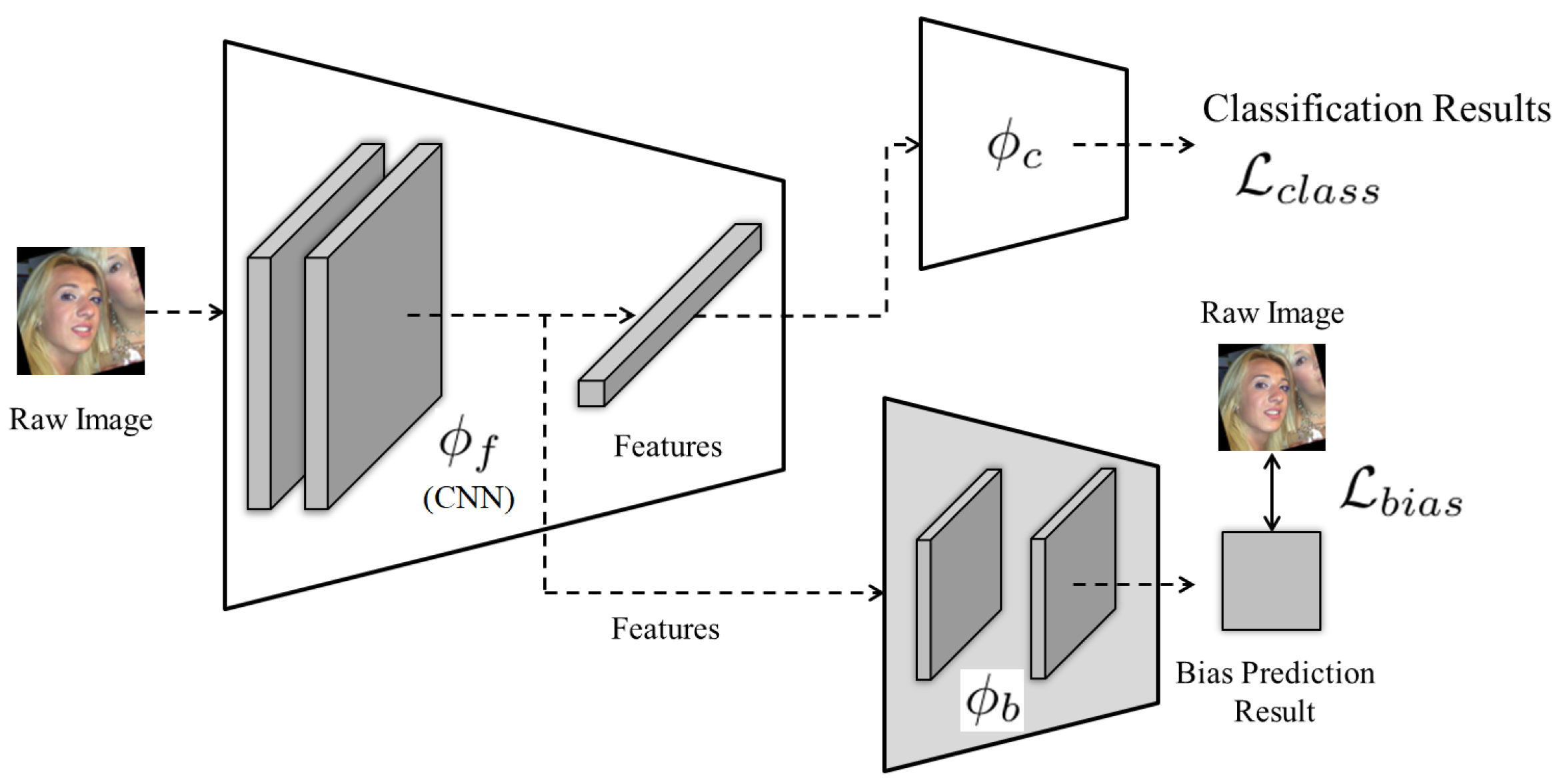
In supervised learning, having a larger number of training samples typically results in lower dataset bias. However, in few-shot image classification, where only five or fewer training samples are available per task, the likelihood of dataset bias in the training set significantly increases. This can lead to the model learning to incorporate the bias as important information, which can negatively impact its performance on new data. To alleviate this issue, the model requires an additional mechanism that can facilitate embedding of features that exclude the bias. To address this, we propose a bias prediction network, focusing particularly on color bias, as illustrated in Figure 1. Our approach can be extended to other types of bias that can be represented as predictive targets. We train the bias prediction network to recover the bias of the raw image, such as color, from the embedded features. If the bias prediction network is able to almost fully recover the color bias, the embedded features are assumed to be highly dependent on the color components of the raw samples, indicating the presence of color bias in the features. Conversely, if the model is trained to embed features that are difficult for the bias prediction network to recover from, the bias in the embedded features can be reduced. This can result in a performance improvement of few-shot image classification. It implies that incorporating the bias prediction network into few-shot learning task can contribute to a performance improvement in various real-world applications where biased datasets are prevalent, including VR/AR systems and computer vision applications. This approach will not only help improve model performance but will also ensure that the models are fair and unbiased in their decision making, providing more reliable and trustworthy results.
The major contributions of this study are summarized as follows:
  • We present a novel approach for few-shot image classification that utilizes adversarial learning to train a bias prediction network. Since only a few samples are available for each class, our approach accounts for the presence of color bias in each label, and aims to minimize its impact on classification.
  • The proposed network is compatible with other models and can be easily integrated with them.
  • Our experiments demonstrate that incorporating the bias prediction network into few-shot learning model improves the performance, indicating the potential of our proposed approach to enhance other few-shot learning tasks across various domains.

2. Related Works

2.1. Few-Shot Learning

Few-shot learning (FSL) is a challenging research area that focuses on training models to learn new concepts or classes from only a few examples. One of the popular topics of FSL is few-shot image classification (FSIC), which classify images using FSL methods.
Generally, FSIC is accomplished through meta-learning. The FSIC model is trained using a chain of training tasks, with each task containing only a few data samples. The FSIC problem is known as N-way K-shot problem, where N represents the number of classes (labels), and K represents the number of data samples from each class. Each training task consists of a support set and a query set. The support set is used to learn to classify accurately and is formed by randomly selecting N classes and K data samples from each class, resulting in an N × K support set. In addition, to form the query set, some data points are randomly selected from the N classes, but none of these points should be identical to any data in the support set. The query set is then used to evaluate the performance of the model on the task.
During the training process, the FSIC model extracts features from the support set and generates classifiers. The model evaluates its performance on the query set and updates its parameters accordingly. In the next task, the model randomly selects N new classes, and the evaluation and updating process is repeated. Finally, the model is tested on data from classes that were not included in the training set. Despite not having learned these new classes before, the model can accurately classify the data.
The FSIC models can be categorized into two groups: distance-based methods and graph-based methods. Distance-based methods compare two feature vectors using metrics such as the L1 distance. One example is the Siamese network [1], which extracts feature vectors from pairs of images randomly selected from the support set and then compares them using a trainable L1 distance. On the other hand, matching networks [25] learn the distance function between the support vectors and the query vector. Prototypical networks [2] embed images to extract feature vectors and calculate the prototype vector for each class. Then, when a feature vector is extracted from a query image, the image is classified as belonging to the class whose prototype vector is the closest.
Graph-based methods, such as the Graph Neural Network (GNN) model [26], represent each image as a node, with edges connecting nodes based on the similarities between their corresponding feature vectors. The edge weights are employed to compute the weighted average vector of the neighboring nodes along with their respective features. This weighted average vector is then aggregated with the node feature vector. EGNN [27] also utilizes the GNN architectures, where each edge between two nodes has the value of the similarity between the two nodes, and predicts whether the two images belong to the same class. Recently, methods focusing on classifiers have also been studied. MetaOptNet [6] utilizes linear classifiers trained using a linear support vector machine (SVM).

2.2. Bias Prediction

Dataset bias refers to a situation where the data are not a true representation of the real-world situation or phenomenon that the model is intended to learn from, which can lead to biased predictions or incorrect inferences. Dataset bias can occur due to many reasons, such as the way the data was collected, the characteristics of the study population, or the limitations of the measurement tools. For example, a facial analysis dataset that is largely composed of lighter-skinned subjects may cause errors when analyzing darker-skinned subjects [28]. It is important to identify and minimize dataset bias to ensure that machine learning models are fair, accurate, and reliable.
Bias prediction is a method used to predict bias in a dataset and mitigate the impact of bias in a dataset. One approach to bias prediction utilized generative adversarial networks [29], as demonstrated in a previous study [30]. If dataset bias exists, the labels can be predicted based on the biased samples. This means that the mutual information between the bias of the training samples and labels will be high, indicating that the corresponding labels are closely related to the dataset bias. For instance, if the dataset bias is a biased color distribution (e.g., human face skins in samples are all white or black), we can calculate the entropy of the embedded features from the feature embedding networks. If the bias prediction results reveal a clear color distribution of the training samples, the entropy will be low. Conversely, if a clear color distribution cannot be found, the entropy will be high. Therefore, the networks are trained to maximize entropy resulting in reducing the effects of color bias. Another approach, Just Train Twice (JTT) [20], is also a straightforward method that mitigates the dataset bias. The algorithm of JTT consists of two stages: identification and upweighting. In the first stage, the framework collects misclassified data from its identification model and makes an error set. Then, in the second stage, the framework upweights the error set and trains the final model using the training data with the upweighted error set. Data augmentation could be a solution for dataset bias. The method proposed in [21] attempts to weaken the correlations among two or more attributes. For example, in the human face dataset, a person wearing a hat tends to also wear glasses. Thus, the method generates images with persons only wearing either a hat or glasses. In this way, the dataset bias in the attributes can be mitigated.
Overall, the few-shot image classification model is able to classify unseen classes, making it beneficial in many practical scenarios where acquiring a large amount of labeled data is not feasible. However, the common issue of dataset bias is required to be addressed to ensure generalization to diverse data domains. Our approach aims to improve the performance of few-shot classification tasks, despite the presence of biased samples in the dataset.

3. Algorithm

3.1. The Bias Prediction Network

Consider a given training set X = x i , y i i = 1 N , where x i R d represents the i-th image in the set, and y i Y is the corresponding label associated with the image. Few-shot image classification models typically consist of two deep neural networks: a feature embedding network and a classifier. The feature embedding network, denoted as ϕ f extracts features from the raw image. The classifier, denoted as ϕ c , takes the extracted features as input and outputs the classification result. The output of the feature embedding network for a raw image data x is denoted as ϕ f ( x ) . The classification result can be expressed as ϕ c ϕ f ( x ) .
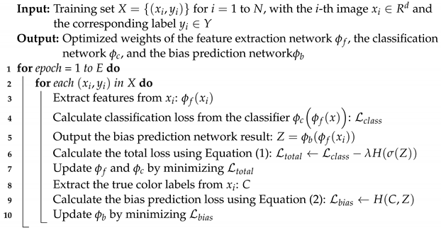
Here, we detail the incorporation of our novel bias prediction network into the original networks ϕ f and ϕ c , as well as its role within the overall model. We note that the original networks ϕ f and ϕ c represent the few-shot image classification model. The overall architecture is illustrated in Figure 2, and the pseudo code is described in Algorithm 1. Our proposed bias prediction network, denoted as ϕ b , is designed to take the embedded features generated by ϕ f as input. The output from the bias prediction network, ϕ b ϕ f ( x ) , is subsequently passed through a softmax function. We define the output before the softmax function as Z, and the output after the softmax as σ ( Z ) = σ ϕ b ϕ f ( x ) , where σ signifies the softmax function.
Algorithm 1: Networks optimization with the bias prediction network
Electronics 12 02470 i001
We are particularly focused on color bias and prioritize the independence between the color distribution of the input and the corresponding features. Therefore, the bias prediction network is designed to evaluate the dependency between the color distribution and the features and this evaluation is achieved by computing cross-entropy between the color distribution and the output of the bias prediction network, which is described in Section 3.3. If the cross-entropy is low, the distribution and the output are correlated, which means that the distribution and the features are dependent. On the other hand, if the cross-entropy is high, it can be assumed that the distribution and the features are barely dependent.
Although we utilize the bias prediction network architecture proposed in [30], we specifically target color bias within the context of few-shot image classification. Our network predicts color bias and is designed to be compatible with various existing few-shot image classification models. This aligns with our belief that color distribution in a dataset, including attributes such as skin or hair color, represents a prevalent form of dataset bias. In scenarios where the attribute we aim to classify has minimal connection with colors, the features extracted by ϕ f show no correlation with colors. As such, our bias prediction network is tasked with not only predicting but also alleviating this color bias. Furthermore, our proposed network is compatible with various existing few-shot image classification models, allowing for broad applicability.
The algorithm introduces two main loss functions: the total loss L t o t a l and the bias prediction loss L b i a s . The classification loss, denoted as L c l a s s , is computed from the classifier ϕ c ϕ f ( x ) , which signifies the result of few-shot image classification and is used to compute the total loss L t o t a l . First, we calculate L t o t a l and update the original model ( ϕ f and ϕ c ). Subsequently, we calculate L b i a s and update ϕ b . These loss functions are interactively updated during the training procedure.

3.2. The Total Loss

The total loss function is defined as:
L t o t a l = L c l a s s λ H σ ( Z ) ,
where L c l a s s is the classification loss, H ( · ) is the entropy function, and λ is the hyperparameter for entropy regularization. We note that the classification loss, L c l a s s , is pre-defined by the original few-shot classification model and is typically represented as a cross-entropy function. The goal of this loss function is to encourage the feature embedding network ϕ f to generate features that are less dependent on the color distribution of the input image. Specifically, the output of the bias prediction network ϕ b , denoted as σ ( Z ) , represents the color labels of a resized image that the network recovers from the embedded features. If the entropy of the output σ ( Z ) is low, it means that the bias prediction network can easily predict the colors of the resized image from the embedded feature, indicating that the features highly depend on the color distribution of the input image. By maximizing the entropy of the output of the bias prediction network H σ ( Z ) , we can encourage the feature embedding network to generate features that are less dependent on the color distribution of the input image, resulting in a more robust and generalizable model.

3.3. The Bias Prediction Loss

Predicting dataset bias is critical when the features of a dataset fail to accurately represent the corresponding class labels. An example is a dataset where most cats have white hair, and most dogs have black hair. In such cases, the model’s performance would be poor when predicting the colors of cats and dogs with other hair colors. This is because hair color alone is not sufficient to represent cats and dogs. Consequently, when the features of a dataset are not representative of the classes, it can lead to incorrect and unreliable predictions.
In this study, we aim to predict color bias in raw images. Due to the limited number of training samples, it is challenging to represent all possible colors for each object. Therefore, we assume that a color bias exists for each label and design the bias prediction network ϕ b to recover the color components of the input image from the embedded features. To evaluate the performance of the bias prediction network, we compare the color labels of the resized raw image and the output σ ( Z ) of the network. The bias prediction loss is defined using a cross-entropy function:
L b i a s = H C , Z ,
where H ( · , · ) denotes a cross-entropy function and C is a matrix of true color labels.
Figure 3 presents the detailed architecture of the bias prediction network and how the network trained with respect to the color bias. Assuming that the output of the feature embedding network is 128 × 21 × 21 , the features are passed through two CNN layers to obtain the bias prediction results with a size of 8 × 21 × 21 . To compare the predicted color bias with the true color labels, the sizes of both are matched. Consequently, both the height and the width of the predicted results are resized to 21 pixels. To accommodate the range of values of the red, green, and blue channels, a color binning technique is applied to split the range into eight equal intervals ( [ 0 , 31 ] , [ 32 , 63 ] , , [ 224 , 255 ] ). The compressed data of the raw images are represented by C.
The bias prediction loss in Equation (2) is calculated using the following equation:
L b i a s = L b i a s ( r e d ) + L b i a s ( g r e e n ) + L b i a s ( b l u e ) 3
L b i a s ( · ) = 1 8 · 21 · 21 i = 1 8 j = 1 21 k = 1 21 c i j k log z i j k ,
where L b i a s ( r e d ) , L b i a s ( g r e e n ) , and L b i a s ( b l u e ) represent the color bias prediction losses for the red, green, and blue channels, respectively, and c i j k and z i j k ( i = 1 , , 8 , j = 1 , , 21 , k = 1 , , 21 ) are elements of C and Z, respectively. The bias prediction loss is calculated as the average of the losses across the three color channels. Each of these losses is determined by the cross-entropy between C for each respective channel and Z.

3.4. Training Procedure

The original networks ϕ f and ϕ c are trained to minimize L t o t a l , whereas the additional bias prediction network ϕ b is trained to minimize L b i a s . The classification loss L c l a s s depends on the loss function of the original networks, while H ( σ ( Z ) ) is related to ϕ b . Meanwhile, L b i a s is evaluated when ϕ b predicts the color labels of the raw image from the embedded features.
In Equation (1), L t o t a l becomes smaller if the entropy H ( σ ( Z ) ) is higher. Therefore, ϕ f attempts to embed features that ϕ b can hardly infer the color component of the raw image. After ϕ f is updated, ϕ b tries to recover the color components of the raw image from the embedded features to minimize L b i a s . Subsequently, ϕ b is updated. This procedure is repeated for another training sample. The corresponding pseudo code is shown in Algorithm 1.

4. Results

4.1. Experimental Setup

Our study aims to enhance the performance of existing few-shot classification models by mitigating color bias. To demonstrate the effectiveness of our proposed bias prediction (BP) network, we compare the performances of multiple existing models both with and without integrating the BP network. We evaluated the performance of existing few-shot classification models, such as EGNN [27], MetaOptNet [6], DeepEMD [9], and SetFeat [31], using four benchmark datasets as follows:
  • miniImageNet [25] is the most general few-shot learning dataset. This is derived from the ILSVRC-12 dataset [32]. All images have a size of 84 × 84 pixels. The dataset has 100 classes, and each class has 600 image samples.
  • CIFAR100 Few-Shots (CIFAR-FS) [33] is randomly split from CIFAR-100 [34] dataset. It consists of 64 training classes, 16 validation classes, and 20 test classes. The classes contain 600 images per class. Each image has a resolution of 32 × 32 pixels.
  • Fewshot-CIFAR100 (FC-100) [35] is another split dataset from CIFAR-100 for few-shot learning. It contains 12 categories for training, 4 categories for validation, and 4 categories for tests. Furthermore, there are 60, 20, and 20 low-level classes, respectively, and each class has 600 images of size 32 × 32 pixels.
  • Adience [16] contains about 20,000 human face images with various genders, ages, and races. All images are aligned, and have a size of 84 × 84 pixels. To perform more difficult classification tasks, we divide the data into two or four age groups: Infant (approximately 0–2 years old), Juvenile (8–12 years old), Young (25–32 years old), and Old (60–100 years old).

4.2. Effectiveness of BP on Multiple Few-Shot Learning Models and Datasets

In this section, we present the experimental results obtained from our study where we applied the BP network to several existing few-shot classification models, which are mentioned above. The study evaluated the effectiveness of the bias prediction network across multiple benchmark datasets, including miniImageNet, CIFAR-FS, FC-100, and Adience, employing five-way one-shot and five-way five-shot learning settings.
The performance (accuracy) of each dataset and model was evaluated with and without the integration of the bias prediction network. Results presented in Table 1, Table 2 and Table 3 demonstrate that the bias prediction network effectively enhances the performance of most original few-shot learning models in our study. Overall, our study highlights the potential of the bias prediction network as a tool for improving the performance of few-shot classification models where biased samples are prevalent. The results show the importance of considering and addressing bias in the development of few-shot learning models to ensure fairness and accuracy in their predictions.
In order to confirm the statistical significance of performance improvements, we performed a paired t-test comparing the models’ performance between with and without the integration of the Bias Prediction (BP) network. We found that the integration of the BP network substantially improved the performance of few-shot image classification models, yielding statistically significant results (p-value < 0.05). However, we observed an exception with the EGNN model under the miniImageNet dataset in a five-way five-shot learning scenario, where the improvement was not statistically significant (p-value = 0.1872). Despite this, in the five-way one-shot learning on the same dataset, and across all learning tasks in other datasets, the EGNN model showed significant improvements with the integration of the BP network. Therefore, we can conclude that the integration of the BP network generally enhances the performance of few-shot image classification models, including EGNN, under varying conditions and datasets.

4.3. Effectiveness of BP on Skin Color Biased Dataset

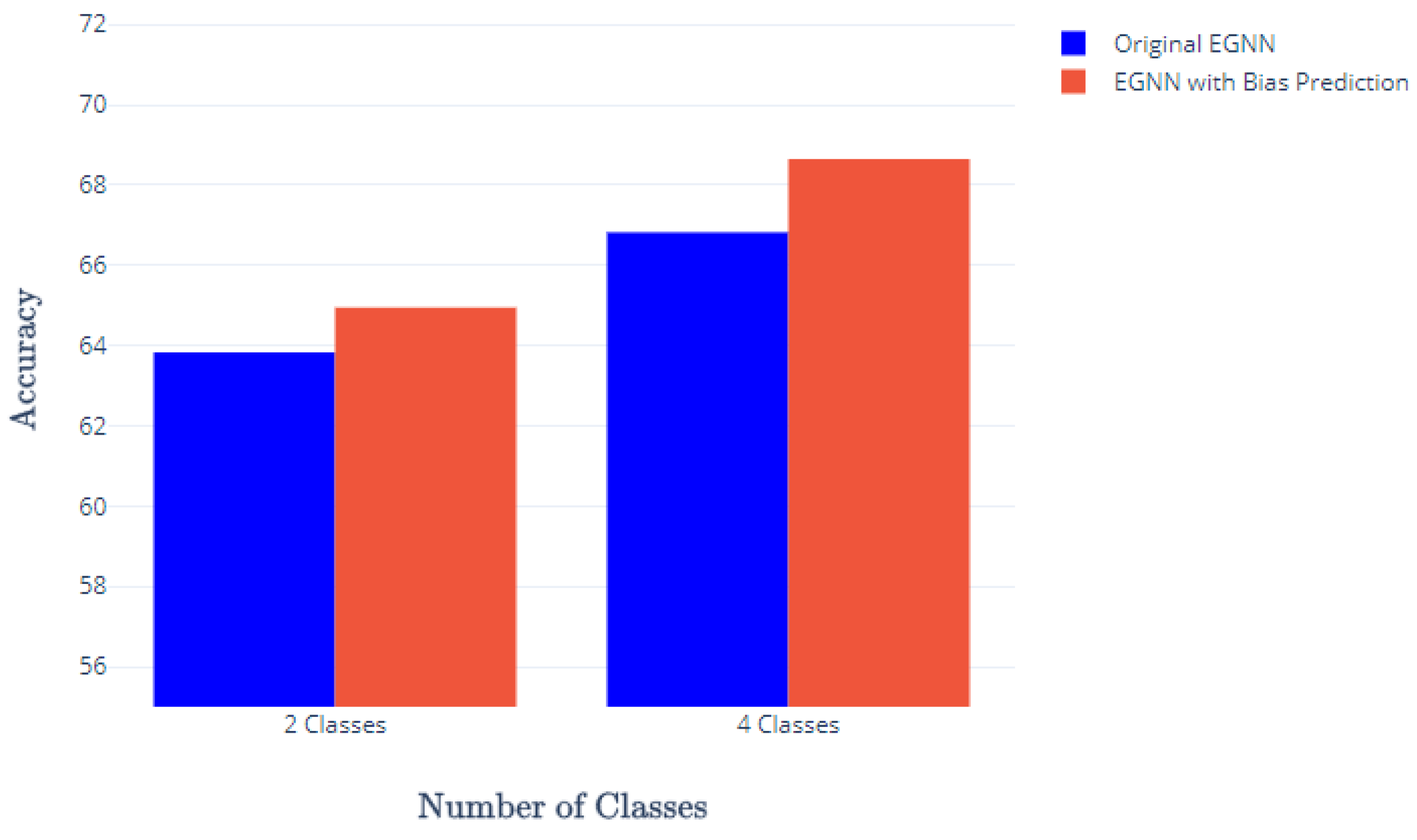
We conducted an additional experiment using the Adience dataset to evaluate the effectiveness of our bias prediction network when the training and test sets were biased by the color of human skin. As illustrated in Figure 1, the training set comprised of young white individuals (white circles) and old black individuals (black circles), while the test set consisted of young black individuals (black squares) and old white individuals (white squares). The task is a two-way five-shot learning problem for classifying young (approximately 25–32 years old) vs. old (approximately 60–100 years old) groups using EGNN as a few-shot learning model. The left part of Figure 4 presents the results, which demonstrate integrating the bias prediction network enhances the performance of EGNN model.
To further investigate the effectiveness of the bias prediction network with more than two classes, we tested with two additional biased classes: Juvenile (approximately 8–12 years old) and Infant (approximately 0–2 years old). We trained the model with the black-skinned Juvenile class and the white-skinned Infant class and tested it with the white-skinned Juvenile class and the black-skinned Infant class, resulting in a four-way five-shot learning task. The right part of Figure 4 shows the results, demonstrating the effectiveness of the bias prediction network in enhancing the original EGNN model’s performance.

4.4. Effectiveness of BP on Color-Filtered Datasets

In this experiment, we demonstrated the effectiveness of the bias prediction network on different color-filtered versions of the miniImageNet dataset. We generated grayscale, red channel, green channel, and blue channel versions of the original dataset, as shown in Figure 5a, and used them during the training stage. The test set consisted of samples from the original dataset, and we evaluated the image classification results on each color-filtered dataset. Some examples of the color-filtered miniImageNet dataset are displayed in Figure 5a. We conducted a few-shot image classification using MetaOptNet as a base model, under the five-way five-shot learning task. The results, presented in Figure 5b, demonstrate that the proposed model with the bias prediction network improved the performance of the model without it ( λ = 0 ) on the red, green, and blue datasets. However, the bias prediction network did not improve the performance on the grayscaled dataset since the color bias of the dataset is significantly reduced when images are grayscaled and all channels have the same value. In most cases, our experiments demonstrated that integrating the bias prediction network resulted in improved performance for various few-shot learning models across multiple datasets, in different scenarios. Overall, our results showed the positive impact of bias prediction network in enhancing the performances of few-shot classification models where biased samples are present.

4.5. Impact of Different Dataset Sizes

In this experiment, we investigated the impact of dataset size on the effectiveness of the bias prediction network in few-shot learning. Since smaller datasets tend to exhibit larger biases, we evaluated the performance of the bias prediction network on the miniImageNet dataset with varying numbers of samples per class: 600, 300, and 100. We experimented with the five-way five-shot learning task and evaluated the performance of EGNN model with and without the bias prediction network. The results presented in Figure 6 indicate that the performance improvement achieved by the bias prediction network was most significant when the number of samples per class was smallest (100 samples). Our findings suggest that datasets with fewer samples per class have a higher likelihood of exhibiting color bias, and the integration of the bias prediction network can be especially effective in mitigating such bias, even in datasets with significant bias.

5. Conclusions

In this work, we addressed the challenge of reducing bias for few-shot learning. To tackle this problem, we proposed a bias prediction network model with the application of few-shot image classification, focusing on color bias. Our approach utilizes adversarial learning to train a bias prediction network that the feature embedding network generate features from input images, which are then fed into the bias prediction network to recover the color labels of the original image. If the training set is color biased, the feature embeddings are likely to be highly dependent on the color values of the training samples, making it easy for the bias prediction network to recover the original image. Accordingly, we introduced a loss function that encourages the feature embedding network to produce embeddings that are less dependent on the color values. Our experimental results demonstrate that the proposed bias prediction network is effective in improving the performance of various existing few-shot learning models across multiple benchmark datasets. The findings suggest that the proposed model has the potential to enhance other few-shot learning tasks across various domains where the number of samples is limited, and biased datasets are prevalent.

Author Contributions

Writing—original draft, J.W.K.; Writing—review and editing, S.Y.K. and K.-A.S.; Supervision, K.-A.S. All authors have read and agreed to the published version of the manuscript.

Funding

This work was supported by the National Research Foundation of Korea (NRF) grant funded by the Korea government (MSIT) (NRF-2022R1A2C1007434) and also under Grant 2021-0-02068 (Artificial Intelligence Innovation Hub), supervised by the IITP (Institute for Information & Communications Technology Planning & Evaluation). The publication fee was supported by the BK21 FOUR program of the NRF of Korea funded by the Ministry of Education (NRF5199991014091).

Data Availability Statement

Publicly available datasets were analyzed in this study. This data can be found here: https://www.kaggle.com/datasets/arjunashok33/miniimagenet (accessed on 27 May 2023); https://github.com/bertinetto/r2d2 (accessed on 27 May 2023); https://github.com/ServiceNow/TADAM (accessed on 27 May 2023); https://talhassner.github.io/home/projects/Adience/Adience-data.html (accessed on 27 May 2023).

Conflicts of Interest

The authors declare no conflict of interest.

References

  1. Koch, G.; Zemel, R.; Salakhutdinov, R. Siamese neural networks for one-shot image recognition. In Proceedings of the ICML Deep Learning Workshop, Lille, France, 6–11 July 2015; Volume 2. [Google Scholar]
  2. Snell, J.; Swersky, K.; Zemel, R. Prototypical Networks for Few-shot Learning. In Proceedings of the Advances in Neural Information Processing Systems, Long Beach, CA, USA, 4–9 December 2017; Guyon, I., Luxburg, U.V., Bengio, S., Wallach, H., Fergus, R., Vishwanathan, S., Garnett, R., Eds.; Curran Associates, Inc.: Red Hook, NY, USA, 2017; Volume 30. [Google Scholar]
  3. Sung, F.; Yang, Y.; Zhang, L.; Xiang, T.; Torr, P.H.; Hospedales, T.M. Learning to Compare: Relation Network for Few-Shot Learning. In Proceedings of the IEEE/CVF Conference on Computer Vision and Pattern Recognition (CVPR), Salt Lake City, UT, USA, 18–23 June 2018; pp. 1199–1208. [Google Scholar] [CrossRef]
  4. Ren, M.; Ravi, S.; Triantafillou, E.; Snell, J.; Swersky, K.; Tenenbaum, J.B.; Larochelle, H.; Zemel, R.S. Meta-Learning for Semi-Supervised Few-Shot Classification. In Proceedings of the International Conference on Learning Representations, Vancouver, BC, Canada, 30 April–3 May 2018. [Google Scholar]
  5. Rusu, A.A.; Rao, D.; Sygnowski, J.; Vinyals, O.; Pascanu, R.; Osindero, S.; Hadsell, R. Meta-Learning with Latent Embedding Optimization. In Proceedings of the International Conference on Learning Representations, New Orleans, LA, USA, 6–9 May 2019. [Google Scholar]
  6. Lee, K.; Maji, S.; Ravichandran, A.; Soatto, S. Meta-Learning with Differentiable Convex Optimization. In Proceedings of the IEEE/CVF Conference on Computer Vision and Pattern Recognition (CVPR), Long Beach, CA, USA, 15–20 June 2019. [Google Scholar]
  7. Chu, W.H.; Li, Y.J.; Chang, J.C.; Wang, Y.C.F. Spot and learn: A maximum-entropy patch sampler for few-shot image classification. In Proceedings of the IEEE/CVF Conference on Computer Vision and Pattern Recognition, Long Beach, CA, USA, 15–20 June 2019; pp. 6251–6260. [Google Scholar]
  8. Li, X.; Sun, Q.; Liu, Y.; Zhou, Q.; Zheng, S.; Chua, T.S.; Schiele, B. Learning to Self-Train for Semi-Supervised Few-Shot Classification. In Proceedings of the Advances in Neural Information Processing Systems, Vancouver, BC, Canada, 8–14 December 2019; Wallach, H., Larochelle, H., Beygelzimer, A., d’Alché-Buc, F., Fox, E., Garnett, R., Eds.; Curran Associates, Inc.: Red Hook, NY, USA, 2019; Volume 32. [Google Scholar]
  9. Zhang, C.; Cai, Y.; Lin, G.; Shen, C. DeepEMD: Few-Shot Image Classification with Differentiable Earth Mover’s Distance and Structured Classifiers. In Proceedings of the IEEE/CVF Conference on Computer Vision and Pattern Recognition, Seattle, WA, USA, 13–19 June 2020; pp. 12203–12213. [Google Scholar]
  10. Medina, C.; Devos, A.; Grossglauser, M. Self-Supervised Prototypical Transfer Learning for Few-Shot Classification. arXiv 2020, arXiv:2006.11325. [Google Scholar]
  11. Tian, P.; Yu, H.; Xie, S. An Adversarial Meta-training Framework for Cross-domain Few-Shot Learning. IEEE Trans. Multimed. 2022, 24, 1–12. [Google Scholar] [CrossRef]
  12. Xing, C.; Rostamzadeh, N.; Oreshkin, B.N.; Pinheiro, P.O. Adaptive Cross-Modal Few-Shot Learning. In Proceedings of the 33rd International Conference on Neural Information Processing Systems, Vancouver, BC, Canada, 8–14 December 2019; Curran Associates Inc.: Red Hook, NY, USA, 2019. [Google Scholar]
  13. Chen, X.; Yao, L.; Zhou, T.; Dong, J.; Zhang, Y. Momentum contrastive learning for few-shot COVID-19 diagnosis from chest CT images. Pattern Recognit. 2021, 113, 107826. [Google Scholar] [CrossRef] [PubMed]
  14. Shao, H.; Zhong, D. Few-shot palmprint recognition via graph neural networks. Electron. Lett. 2019, 55, 890–892. [Google Scholar] [CrossRef]
  15. Lemke, C.; Budka, M.; Gabrys, B. Metalearning: A survey of trends and technologies. Artif. Intell. Rev. 2015, 44, 117–130. [Google Scholar] [CrossRef] [PubMed]
  16. Eidinger, E.; Enbar, R.; Hassner, T. Age and gender estimation of unfiltered faces. IEEE Trans. Inf. Forensics Secur. 2014, 9, 2170–2179. [Google Scholar] [CrossRef]
  17. Orphanou, K.; Otterbacher, J.; Kleanthous, S.; Batsuren, K.; Giunchiglia, F.; Bogina, V.; Tal, A.S.; Hartman, A.; Kuflik, T. Mitigating Bias in Algorithmic Systems—A Fish-Eye View. ACM Comput. Surv. 2022, 55, 1–37. [Google Scholar] [CrossRef]
  18. Mehrabi, N.; Morstatter, F.; Saxena, N.; Lerman, K.; Galstyan, A. A Survey on Bias and Fairness in Machine Learning. ACM Comput. Surv. 2021, 54, 1–35. [Google Scholar] [CrossRef]
  19. Wang, Z.; Qinami, K.; Karakozis, I.C.; Genova, K.; Nair, P.; Hata, K.; Russakovsky, O. Towards Fairness in Visual Recognition: Effective Strategies for Bias Mitigation. In Proceedings of the IEEE/CVF Conference on Computer Vision and Pattern Recognition (CVPR), Seattle, WA, USA, 13–19 June 2020. [Google Scholar]
  20. Liu, E.Z.; Haghgoo, B.; Chen, A.S.; Raghunathan, A.; Koh, P.W.; Sagawa, S.; Liang, P.; Finn, C. Just train twice: Improving group robustness without training group information. In Proceedings of the International Conference on Machine Learning, PMLR, Online, 18–24 July 2021; pp. 6781–6792. [Google Scholar]
  21. Ramaswamy, V.V.; Kim, S.S.Y.; Russakovsky, O. Fair Attribute Classification Through Latent Space De-Biasing. In Proceedings of the IEEE/CVF Conference on Computer Vision and Pattern Recognition (CVPR), Nashville, TN, USA, 20–25 June 2021; pp. 9301–9310. [Google Scholar]
  22. Mondal, I.; Sen, P.; Ganguly, D. Multi-objective few-shot learning for fair classification. In Proceedings of the 30th ACM International Conference on Information & Knowledge Management, Gold Coast, Australia, 1–5 November 2021; pp. 3338–3342. [Google Scholar]
  23. Bennequin, E.; Tami, M.; Toubhans, A.; Hudelot, C. Few-Shot Image Classification Benchmarks are Too Far From Reality: Build Back Better with Semantic Task Sampling. In Proceedings of the IEEE/CVF Conference on Computer Vision and Pattern Recognition, New Orleans, LA, USA, 18–24 June 2022; pp. 4767–4776. [Google Scholar]
  24. Ghaffari, S.; Saleh, E.; Forsyth, D.; Wang, Y.X. On the Importance of Firth Bias Reduction in Few-Shot Classification. In Proceedings of the International Conference on Learning Representations, Online, 25–29 April 2022. [Google Scholar]
  25. Vinyals, O.; Blundell, C.; Lillicrap, T.; kavukcuoglu, K.; Wierstra, D. Matching Networks for One Shot Learning. In Proceedings of the Advances in Neural Information Processing Systems, Barcelona, Spain, 5–10 December 2016; Lee, D., Sugiyama, M., Luxburg, U., Guyon, I., Garnett, R., Eds.; Curran Associates, Inc.: Red Hook, NY, USA, 2016; Volume 29. [Google Scholar]
  26. Satorras, V.G.; Estrach, J.B. Few-Shot Learning with Graph Neural Networks. In Proceedings of the International Conference on Learning Representations, Vancouver, BC, Canada, 30 April–3 May 2018. [Google Scholar]
  27. Kim, J.; Kim, T.; Kim, S.; Yoo, C.D. Edge-Labeling Graph Neural Network for Few-Shot Learning. In Proceedings of the IEEE/CVF Conference on Computer Vision and Pattern Recognition (CVPR), Long Beach, CA, USA, 15–20 June 2019. [Google Scholar]
  28. Buolamwini, J.; Gebru, T. Gender shades: Intersectional accuracy disparities in commercial gender classification. In Proceedings of the Conference on Fairness, Accountability and Transparency, PMLR, New York, NY, USA, 23–24 February 2018; pp. 77–91. [Google Scholar]
  29. Goodfellow, I.; Pouget-Abadie, J.; Mirza, M.; Xu, B.; Warde-Farley, D.; Ozair, S.; Courville, A.; Bengio, Y. Generative Adversarial Nets. In Proceedings of the Advances in Neural Information Processing Systems, Montreal, QC, Canada, 8–13 December 2014; Ghahramani, Z., Welling, M., Cortes, C., Lawrence, N., Weinberger, K.Q., Eds.; Curran Associates, Inc.: Red Hook, NY, USA, 2014; Volume 27. [Google Scholar]
  30. Kim, B.; Kim, H.; Kim, K.; Kim, S.; Kim, J. Learning not to learn: Training deep neural networks with biased data. In Proceedings of the IEEE/CVF Conference on Computer Vision and Pattern Recognition, Long Beach, CA, USA, 15–20 June 2019; pp. 9012–9020. [Google Scholar]
  31. Afrasiyabi, A.; Larochelle, H.; Lalonde, J.F.; Gagné, C. Matching feature sets for few-shot image classification. In Proceedings of the IEEE/CVF Conference on Computer Vision and Pattern Recognition, New Orleans, LA, USA, 18–24 June 2022; pp. 9014–9024. [Google Scholar]
  32. Russakovsky, O.; Deng, J.; Su, H.; Krause, J.; Satheesh, S.; Ma, S.; Huang, Z.; Karpathy, A.; Khosla, A.; Bernstein, M.; et al. Imagenet large scale visual recognition challenge. Int. J. Comput. Vis. 2015, 115, 211–252. [Google Scholar] [CrossRef]
  33. Bertinetto, L.; Henriques, J.; Torr, P.; Vedaldi, A. Meta-learning with differentiable closed-form solvers. In Proceedings of the International Conference on Learning Representations, New Orleans, LA, USA, 6–9 May 2019. [Google Scholar]
  34. Krizhevsky, A.; Hinton, G. Learning Multiple Layers of Features from Tiny Images. Technical Report, Toronto, ON, Canada, 2009. Available online: http://www.cs.utoronto.ca/~kriz/learning-features-2009-TR.pdf (accessed on 27 May 2023).
  35. Oreshkin, B.; Rodríguez López, P.; Lacoste, A. Tadam: Task dependent adaptive metric for improved few-shot learning. In Proceedings of the Advances in Neural Information Processing Systems, Montreal, QC, Canada, 3–8 December 2018; Volume 31. [Google Scholar]
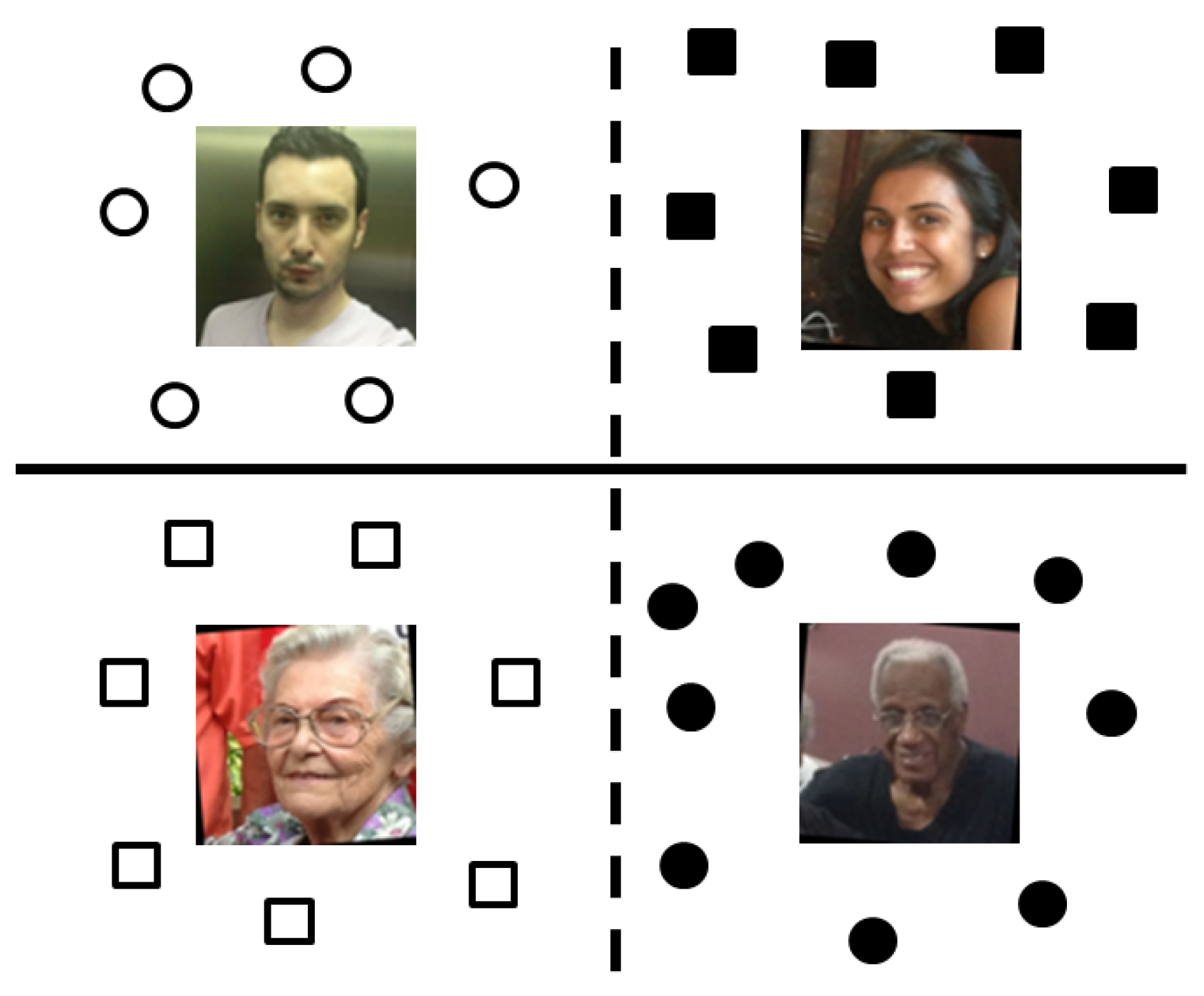
Figure 1. An illustration of the impact of dataset bias on few-shot image classification. It depicts a feature space with images of faces of people with varying ages. White and black circles indicate the training samples, and white and black squares indicate the test samples. A model is trained to classify whether each face is young or old. The solid line represents the desirable classifier. It indicates that the classification performance will be poor if the model is trained to classify according to the dotted line, which is biased.
Electronics 12 02470 g001
Figure 2. The overall architecture comprises a feature embedding network ϕ f , a classification network ϕ c , and a bias prediction network ϕ b followed by ϕ f . We note that ϕ f represents a CNN architecture and the features embedded by ϕ f are fed as an input to the bias prediction network, which outputs the bias prediction result. Based on the result, the bias prediction loss L b i a s is obtained by computing the cross-entropy between the resized raw image and the bias prediction result. Meanwhile, the classification loss L c l a s s is calculated by the original model and is used to compute the total loss L t o t a l . The image samples used in this architecture are from the Adience dataset.
Electronics 12 02470 g002
Figure 3. The detailed architecture of the bias prediction network ϕ b for predicting color bias involves several steps. First, a raw input image is resized and split into three color channels. Next, the pixel values of each channel are grouped into eight intervals to match the size of the output of the bias prediction network. Then, the bias prediction loss is calculated by computing the negative cross-entropy between the output generated by the network and the true color labels of the resized image. A higher bias prediction loss indicates that the model is less successful in predicting the color bias, which leads to a higher total loss. The bias prediction loss encourages the model to learn features that are less dependent on the color distribution of the input image.
Electronics 12 02470 g003
Figure 4. The effectiveness of the bias prediction network on the biased Adience dataset with the EGNN model. We evaluated the performance of the few-shot classification model EGNN with and without the bias prediction network on the Adience dataset containing biased data. The classification performance (accuracy) is represented on the vertical axis and the number of classes on the horizontal axis. The results showed the addition of bias prediction network improved the performance of the original EGNN across different number of classes. This result highlights the effectiveness of the bias prediction network in addressing color bias in a few-shot classification task.
Electronics 12 02470 g004
Figure 5. The examples of the color-filtered miniImageNet datasets and the experimental results for each dataset. (a) Examples of the color-filtered versions of miniImageNet dataset. The first row displays the grayscaled version of the original examples, and the second, third, and fourth rows show the red, green, and blue channel images of the examples, respectively. (b) Performance of the bias prediction network on the color-filtered miniImageNet dataset. MetaOptNet was used as the base model. The horizontal axis represents the bias prediction coefficient λ in Equation (1), while the vertical axis represents the improvement in performance by the bias prediction network.
Electronics 12 02470 g005
Figure 6. Performance of the bias prediction network with varying number of samples per class in the miniImageNet dataset. We evaluated the prediction performance using EGNN. The horizontal axis represents the number of the samples of each class. The vertical axis represents accuracy with and without the bias prediction network. The results indicate that the bias prediction network had the greatest impact on datasets with a smaller number of samples per class.
Electronics 12 02470 g006
Table 1. Performance comparison of few-shot classification models with and without the bias prediction network on miniImageNet datasets.
ModelsFive-Way One-ShotFive-Way Five-Shot
OriginalBP AddedOriginalBP Added
EGNN 46.68 ± 0.28 % 47.14 ± 0.22 % 61.50 ± 0.09 % 61.24 ± 0.10 %
MetaOptNet 54.68 ± 0.10 % 56.06 ± 0.20 % 71.07 ± 0.07 % 71.19 ± 0.13 %
DeepEMD 63.77 ± 0.12 % 64.57 ± 0.24 % 79.43 ± 0.09 % 79.99 ± 0.27 %
SetFeat 67.33 ± 0.29 % 68.75 ± 0.39 % 82.61 ± 0.55 % 83.08 ± 0.74 %
Table 2. Performance comparison of few-shot classification models with and without the bias prediction network on CIFAR-FS datasets.
ModelsFive-Way One-ShotFive-Way Five-Shot
OriginalBP AddedOriginalBP Added
EGNN 51.69 ± 0.13 % 52.89 ± 0.25 % 64.86 ± 0.24 % 65.23 ± 0.36 %
MetaOptNet 59.58 ± 0.20 % 61.10 ± 0.40 % 73.61 ± 0.26 % 73.87 ± 0.71 %
DeepEMD 64.41 ± 0.23 % 65.88 ± 0.35 % 80.05 ± 0.27 % 80.42 ± 0.54 %
SetFeat 68.12 ± 0.18 % 69.05 ± 0.34 % 82.92 ± 0.34 % 83.23 ± 0.72 %
Table 3. Performance comparison of few-shot classification models with and without the bias prediction network on FC-100 datasets.
ModelsFive-Way One-ShotFive-Way Five-Shot
OriginalBP AddedOriginalBP Added
EGNN 32.19 ± 0.08 % 33.55 ± 0.15 % 43.79 ± 0.09 % 44.07 ± 0.18 %
MetaOptNet 34.02 ± 0.10 % 34.72 ± 0.25 % 47.60 ± 0.57 % 47.93 ± 0.82 %
DeepEMD 41.23 ± 0.09 % 42.75 ± 0.15 % 53.43 ± 0.23 % 53.99 ± 0.59 %
SetFeat 42.84 ± 0.20 % 43.64 ± 0.31 % 55.76 ± 0.43 % 55.95 ± 0.52 %
Disclaimer/Publisher’s Note: The statements, opinions and data contained in all publications are solely those of the individual author(s) and contributor(s) and not of MDPI and/or the editor(s). MDPI and/or the editor(s) disclaim responsibility for any injury to people or property resulting from any ideas, methods, instructions or products referred to in the content.