A Joint-Learning-Based Dynamic Graph Learning Framework for Structured Prediction ^†

Abstract

Graph neural networks (GNNs) have achieved remarkable success in structured prediction, owing to the GNNs’ powerful ability in learning expressive graph representations. However, most of these works learn graph representations based on a static graph constructed by an existing parser, suffering from two drawbacks: (1) the static graph might be error-prone, and the errors introduced in the static graph cannot be corrected and might accumulate in later stages, and (2) the graph construction stage and graph representation learning stage are disjoined, which negatively affects the model’s running speed. In this paper, we propose a joint-learning-based dynamic graph learning framework and apply it to two typical structured prediction tasks: syntactic dependency parsing, which aims to predict a labeled tree, and semantic dependency parsing, which aims to predict a labeled graph, for jointly learning the graph structure and graph representations. Experiments are conducted on four datasets: the Universal Dependencies 2.2, the Chinese Treebank 5.1, the English Penn Treebank 3.0 in 13 languages for syntactic dependency parsing, and the SemEval-2015 Task 18 dataset in three languages for semantic dependency parsing. The experimental results show that our best-performing model achieves a new state-of-the-art performance on most language sets of syntactic dependency and semantic dependency parsing. In addition, our model also has an advantage in running speed over the static graph-based learning model. The outstanding performance demonstrates the effectiveness of the proposed framework in structured prediction.

1. Introduction

Structured prediction aims to solve problems, where the output set is not a linear space but rather a set of structured objects such as sequences, trees, or graphs [1,2]. Structured prediction has played a key role in the area of natural language processing (NLP). In many NLP tasks, the outputs are structures that can take the form of sequences (e.g., named entity recognition and semantic role labeling), trees (e.g., constituency parsing and syntactic dependency parsing), or general labeled graphs (e.g., relation extraction, semantic dependency parsing, and abstract meaning representation (AMR) parsing).

Recent works of structured prediction show that graph neural networks (GNNs) can provide a scalable and highly performant means of incorporating linguistic information and other structural biases into NLP models. They have been applied to various kinds of representations (e.g., syntactic trees, semantic graphs, and co-reference structures) and show effectiveness on a range of tasks, including named entity recognition [3,4], semantic role labeling [5], relation extraction [6,7,8], and syntactic and semantic dependency parsing [9,10,11,12].

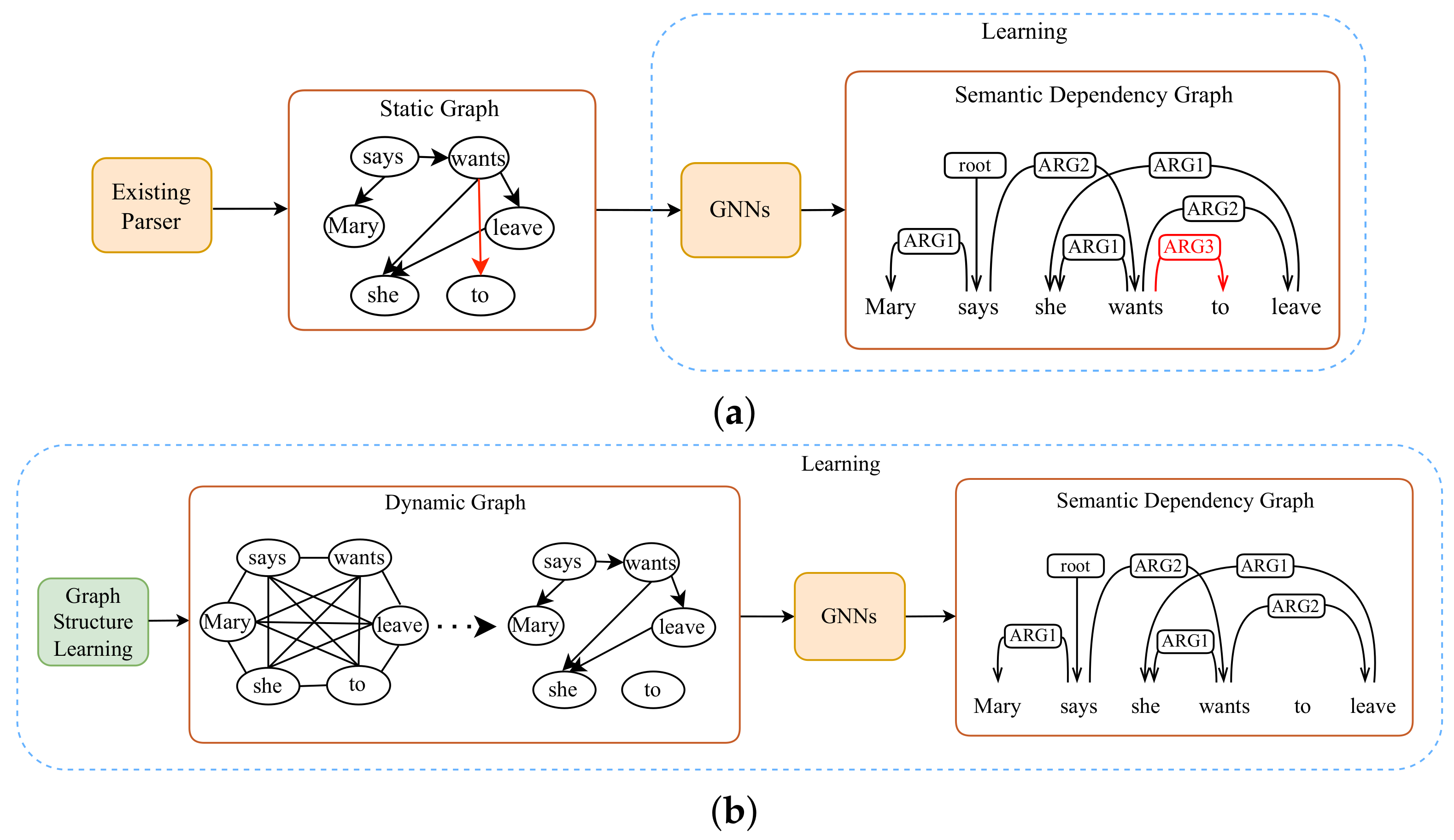
Most of these models utilize an existing parser to construct an initial static graph (e.g., constituency tree, dependency tree, or dependency graph), and then use GNNs to learn node embeddings based on the static graph to predict an objective graph. A static graph-based learning example for semantic dependency parsing is shown as Figure 1. These models have made significant accuracy improvements in the corresponding tasks, owing to the powerful ability of GNNs in learning expressive graph representations.

Despite the promising performance, there are still two drawbacks in these models: (1) the static graph might be error-prone (e.g., noisy or incomplete), and the errors introduced in the static graph cannot be corrected and might accumulate in later stages, and (2) the graph construction stage and graph representation learning stage are disjoined, which negatively affects the model’s running speed.

Recently, several dynamic graph learning approaches have been presented to tackle the above two drawbacks [13,14,15,16]. Most approaches for constructing dynamic graphs aim to learn the graph structure (i.e., a weighted adjacency matrix) in a dynamic fashion, allowing the graph to evolve over time. The graph construction module can be jointly optimized with subsequent graph representation learning modules towards a downstream task in an end-to-end manner.

Inspired by the ideas of these works, we propose a concise and effective dynamic graph learning framework (DynGL) to address the drawbacks of the static graph-based disjoint learning, as shown in Figure 1b, to generate an objective graph from a word sequence rather than an initial static graph. A graph structure learning module is utilized to learn a dynamic graph, and then the learned dynamic graph is fed into the GNNs to learn graph representations. The graph structure learning module and the graph representation learning module are integrated with a joint learning paradigm. Two GNN variants, graph convolutional network (GCN) [17] and graph attention network (GAT), [18] are investigated in the proposed framework.

The DynGL is evaluated on two typical structured prediction tasks: syntactic dependency parsing and semantic dependency parsing. Experiments are conducted on four datasets: the Universal Dependencies (UD) 2.2, the Chinese Treebank (CTB) 5.1, the English Penn Treebank (PTB) 3.0 in 13 languages for syntactic dependency parsing, and the SemEval-2015 Task 18 dataset in three languages for semantic dependency parsing. The experimental results show that our best-performing model outperforms the previous best models by a 0.40% averaged LAS on the UD 2.2, a 0.22% labeled attachment score (LAS) on the PTB 3.0, and a 0.29% averaged Labeled F-measure score (LF1) on the SemEval-2015 Task 18 dataset, respectively, achieving a new state-of-the-art (SOTA) performance on most language sets in syntactic dependency parsing and semantic dependency parsing. In addition, the DynGL shows more advantages with respect to the running speed over the static graph-based learning model. Our code is publicly available at https://github.com/LiBinNLP/DynGL (accessed on 5 April 2023).

The rest of this article is organized as follows. The related works are summarized in Section 2, and the proposed method is described in detail in Section 3. Then, the experiments of syntactic and semantic dependency parsing are presented in Section 4. Next, the analysis of the experimental results is presented in Section 5. Finally, our work is concluded in Section 6.

2. Related Work

In this section, the related studies of structured prediction and dynamic graph learning are summarized as follows.

2.1. Structured Prediction

Structured prediction aims to predict the structured outputs such as sequences, trees, and graphs [1,2]. Many NLP tasks can be viewed as the structured prediction in which the outputs are sequences (e.g., named entity recognition and semantic role labeling), trees (e.g., constituency parsing and syntactic dependency parsing), or general labeled graphs (e.g., relation extraction, semantic dependency parsing, and AMR parsing).

Recent efforts in structured prediction show that GNNs can provide a scalable and highly performant means of incorporating linguistic information and other structural biases into NLP models. GNNs have been applied to learn expressive representations from various kinds of structures (e.g., syntactic trees, semantic graphs, and co-reference structures) and have shown effectiveness on a range of tasks.

Marcheggiani and Titov [5] utilized an existing syntactic dependency parser to construct a dependency tree and then used GCNs to encode it as additional structural knowledge to improve the performance of semantic role labeling. Zhang et al. [19] extended GCNs to make it tailored for pooling information over arbitrary dependency structures produced by an existing parser efficiently in parallel. They applied a novel pruning strategy to the input dependency trees to remove the irrelevant subtrees and incorporated the encoded relevant information into relation extraction to improve it. Guo et al. [8] developed a novel model called attention-guided GCN, which directly takes full dependency trees yielded by an existing parser to improve the relation extraction. Their model can be understood as a soft-pruning approach that automatically learns how to selectively attend to the relevant substructures useful for the relation extraction task. Tang et al. [4] employed GCNs to simultaneously process the word–character-directed acyclic graphs of two directions to produce graph node representations and then incorporated them into the Chinese NER model to enhance it. Zhou et al. [20] integrated syntactic dependency structure information encoded by GCNs with AMR parsing to improve the robustness and generalization ability of models. Jiang and Cohn [21] applied heterogeneous graph attention networks to incorporate the syntactic dependency tree structure and semantic role labeling features of a sentence into co-reference resolutions to build a strong model. Mohammadshahi and Henderson [11] presented a recursive non-autoregressive graph-to-graph transformer architecture and applied it to syntactic dependency parsing. This model used an initialized model to compute an initial graph and then took the initial graph as input and predicted the target graph. Li et al. [12] utilized GNNs to encode an initial semantic dependency graph output by an existing parser to build an effective semantic dependency parser. The higher-order information encoded by GNNs is exceedingly beneficial for improving semantic dependency parsing.

Most of these models utilized an existing parser to construct an initial static structure (e.g., dependency tree and semantic graph) and then used GNNs to learn node embeddings based on the static structure to predict objective structures. These models made significant accuracy improvements in the corresponding tasks and multiple languages, owing to the powerful ability of GNNs in learning expressive graph representations.

Even though these models have achieved promising performance, since the graph construction stage and the graph representation learning stage are disjoined, the errors introduced in the static graph cannot be corrected and might accumulate in later stages. In addition, the disjoined learning paradigm negatively affects the model’s running speed.

2.2. Dynamic Graph Learning

Recent years have witnessed a significantly growing amount of interest in graph learning. Graph learning is the process of learning the representations of a graph; GNNs are the most prominent approaches for graph learning. GNNs take in the original feature and adjacency matrix and output node embeddings as graph representations [17,18,22]. Due to the powerful ability in learning graph representations, GNNs have been applied to various downstream tasks, including node prediction [22], link prediction [23], and graph classification [24].

Despite GNNs’ powerful ability in graph learning, unfortunately, they can only be used when graph-structured data are available. Many NLP tasks may only have sequential data, and there is no graph structure available. To address this limitation, several dynamic graph learning frameworks have been presented, for jointly learning graph structure and graph representations [25].

Chen et al. [13] presented an end-to-end graph learning framework for jointly and iteratively learning the graph structure and graph embedding. The key rationale of their model was to learn a better graph structure based on better node embeddings and, at the same time, to learn better node embeddings based on a better graph structure. Their framework can cope with both transductive and inductive graph learning. Jin et al. [14] presented a general framework that can jointly learn a structural graph and a robust graph neural network model from the perturbed graph based on the fact that adversarial attacks are likely to violate some intrinsic properties (e.g., many real-world graphs are low-rank and sparse, and the features of two adjacent nodes tend to be similar) of a graph. Zhao et al. [15] studied graph data augmentation for GNNs in the context of improving semi-supervised node-classification. They modeled edge weights by taking the inner product of the embeddings of two end nodes with no additional parameters introduced. Sun et al. [16] proposed a novel Variational-Information-Bottleneck-guided graph structure learning framework, namely VIB-GSL, from the perspective of information theory. VIB-GSL is the first attempt to advance the Information Bottleneck principle for graph structure learning, providing a more elegant and universal framework for mining underlying task-relevant relations. The VIB-GSL learns an informative and compressive graph structure to distill the actionable information for specific downstream tasks.

Inspired by the ideas of these works, we propose a dynamic graph learning framework to address the drawbacks of the static graph-based disjoined learning in structured prediction, to generate an objective graph from the word sequence rather than an initial static graph.

3. Methodology

DynGL is a dynamic graph learning model for structured prediction. An overview of DynGL is shown as Figure 2. Given a sentence s with n words $[w_1,w_2,\cdots ,w_n]$, there are four stages to predict its objective graph:

• Contextualized representation learning—a text encoder is used to learn the contextualized representation of each word. Bidirectional long short-term memory network (BiLSTM) and Transformer were explored as the text encoder in our model.
• Graph structure learning—a graph structure learning module is used to learn the adjacency matrix of a potential graph.
• Graph representation learning—the contextualized representations and the learned adjacency matrix are fed into the GNNs to learn expressive node embeddings.
• Edge and label learning—the concatenation of node embeddings and contextualized representations are fed into a biaffine attention-based model to predict the edges and labels.

Figure 2. The overall architecture of the proposed DynGL. The input sentence is first encoded by a text encoder to obtain the contextualized representation. Then, the contextualized representation is input into the graph structure learning module to learn the adjacency matrix. Next, the contextualized representation and the learned adjacency matrix are fed into graph neural networks to obtain the graph node representation. Finally, the contextualized representation and graph node representation are concatenated as the final representation to predict the edge and label by the edge and label prediction components, respectively.

Figure 2. The overall architecture of the proposed DynGL. The input sentence is first encoded by a text encoder to obtain the contextualized representation. Then, the contextualized representation is input into the graph structure learning module to learn the adjacency matrix. Next, the contextualized representation and the learned adjacency matrix are fed into graph neural networks to obtain the graph node representation. Finally, the contextualized representation and graph node representation are concatenated as the final representation to predict the edge and label by the edge and label prediction components, respectively.

3.1. Contextualized Representation Learning

We concatenated the word and feature embeddings and fed them into a text encoder (BiLSTM or Transformer) to obtain contextualized representations.

$$x_i=e_i^{\left(word\right)}\oplus e_i^{\left(feat\right)},$$

(1)

$$c_i=TextEncoder\left(x_i\right),$$

(2)

where $x_i$ is the concatenation (⊕) of the word and feature embeddings of the word $w_i$, and $c_i$ is the contextualized representation of $w_i$.

3.1.1. Word Embedding

One-hundred-dimensional word embeddings from GloVe [26] were used for English; three-hundred-dimensional word embeddings from fasttext [27] were used for the other languages.

3.1.2. Feature Embedding

Five types of feature embeddings were used: (1) Part-of-speech (POS) tag: POS tag embedding $E^{\left(pos\right)}$ was randomly generated, $E^{\left(pos\right)}\in R^{n\times d}$, where n is the number of POS tags; (2) lemma: lemma embedding $E^{\left(lemma\right)}$ was also randomly generated. $E^{\left(lemma\right)}\in R^{l\times d}$, where l is the number of lemmas; (3) character: character embedding was generated using CharLSTM that convolved over three-character embeddings at each time step; (4) BERT: BERT embedding was extracted from the pretrained BERT model [28]; and (5) RoBERTa: RoBERTa embedding was extracted from the pretrained RoBERTa model [29].

3.2. Graph Structure Learning

The purpose of the graph structure learning module is to learn the adjacency matrix A of a potential graph from a complete graph. The distance between two nodes is used to determine whether there is a directed edge between them. The distance between two nodes is usually measured by the metric learning function $\varphi (·,·)$. In this work, the metric learning function $\varphi (·,·)$ was implemented with the attention-based approach. Its architecture is shown as Figure 3.

Two multilayer perceptrons (MLP) were used to capture the representations of the start node and end node, as Equations (3) and (4):

$$h_i^{(adj-start)}=ML{P}^{(adj-start)}\left(c_i\right),$$

(3)

$$h_i^{(adj-end)}=ML{P}^{(adj-end)}\left(c_i\right),$$

(4)

where $h_i^{(adj-start)}$ and $h_i^{(adj-end)}$ are two representations of the word $w_i$ in the start node and the end node computed by $ML{P}^{(adj-start)}$ and $ML{P}^{(adj-end)}$, respectively.

The biaffine attention network (as Equation (5)) was used to compute the score of a possible edge between $w_i$ and $w_j$, as Equation (6):

$$Biaff(x_1,x_2)=x_1^{T}U{x}_2+W(x_1\oplus x_2)+b,$$

(5)

$$s_{i,j}^{\left(adj\right)}=Biaf{f}^{\left(adj\right)}(h_i^{(adj-end)},h_j^{(adj-start)}),$$

(6)

where U, W, and b are learned parameters, and $s_{i,j}^{\left(adj\right)}$ denotes the score of a possible edge between the words $w_i$ and $w_j$.

A directed edge from $w_i$ to $w_j$ exists when ${\widehat{A}}_{ij}$ is 1. ${\widehat{A}}_{ij}$ in $\widehat{A}$ is computed as Equation (7):

$${\widehat{A}}_{i,j}=\left\{\begin{array}{cc}1,\hfill & s_{i,j}^{\left(adj\right)}>0\hfill \\ 0,\hfill & s_{i,j}^{\left(adj\right)}\le 0\hfill \end{array}\right.,$$

(7)

where $\widehat{A}$ is the estimated adjacency matrix, and ${\widehat{A}}_{i,j}$ is a member of $\widehat{A}$.

3.3. Graph Representation Learning

The graph representation learning module utilizes GNNs to learn each word’s representation (i.e., node embedding) that contains graph structure information. GNNs encode node embeddings in a similar incremental manner: one GNN layer encodes information about the immediate neighbors, and the K layers encode K-order neighborhoods (i.e., information about the nodes at most K hops aways).

K-layer GNNs were employed, which take in the contextualized representations and the learned adjacency matrix A and output the embedding matrix of the final layer as node embeddings R. $R^{\left(k\right)}$ in the kth-layer is computed as Equation (8):

$$R^{\left(k\right)}=GNNLaye{r}^{(k-1)}(R^{(k-1)},\widehat{A}),$$

(8)

where $R^{\left(k\right)}$ is the graph node representation in the kth-layer of the GNNs.

When the GNNLayer is implemented in the GCN, the representation of node i in the kth layer $r_i^{\left(k\right)}$ is computed as Equation (9):

$$r_i^{\left(k\right)}=\sigma \left(W\sum _{j\in N\left(i\right)}{r}_j^{(k-1)}+B{r}_i^{(k-1)}\right).$$

(9)

When the GNNLayer is implemented in the GAT, $r_i^{\left(k\right)}$ is computed as Equation (10):

$$r_i^{\left(k\right)}=\sigma \left(W\sum _{j\in N\left(i\right)}{a}_{ij}^{(k-1)}{r}_j^{(k-1)}+B{r}_i^{(k-1)}\right),$$

(10)

where $a_{ij}^{(k-1)}$ is the attention coefficient of node i to its neighbor j at the $(k-1)$th layer, W and B are learned parameters, $N\left(i\right)$ are neighbors of node i, $\sigma$ is an active function, and $r_i^{\left(0\right)}=c_i$.

3.4. Edge and Label Learning

The edge and label learning module follows the biaffine attention-based model [30], which is shown as Figure 4. There were two components: the edge prediction (shown as Figure 4a) and the label prediction (shown as Figure 4b).

For each word $w_i$, the graph node representation and the contextualized representation were concatenated to represent it, as shown in Equation (11). For each of the two components, we used MLP to split the final word representation $z_i$ into two parts: a start node representation and an end node representation, as shown in Equations (12)–(15):

$$z_i=r_i\oplus c_i,$$

(11)

$$h_i^{(edge-start)}=ML{P}^{(edge-start)}\left(z_i\right),$$

(12)

$$h_i^{(label-start)}=ML{P}^{(label-start)}\left(z_i\right),$$

(13)

$$h_i^{(edge-end)}=ML{P}^{(edge-end)}\left(z_i\right),$$

(14)

$$h_i^{(label-end)}=ML{P}^{(label-end)}\left(z_i\right),$$

(15)

where $r_i$ and $c_i$ are the graph node representation and the contextualized representation for the word $w_i$, respectively, $h_i^{(edge-start)}$ and $h_i^{(edge-end)}$ are the two representations of $w_i$ in the edge start node and the edge end node computed by $ML{P}^{(edge-start)}$ and $ML{P}^{(edge-end)}$, respectively, and $h_i^{(label-start)}$ and $h_i^{(label-end)}$ are the two representations of $w_i$ in the label start node and the label end node computed by $ML{P}^{(label-start)}$ and $ML{P}^{(label-end)}$, respectively.

Two biaffine classifiers were used to predict the edges and labels, as Equations (16) and (17):

$$s_{i,j}^{\left(edge\right)}=Biaf{f}^{\left(edge\right)}(h_i^{(edge-end)},h_j^{(edge-start)}),$$

(16)

$$s_{i,j}^{\left(label\right)}=Biaf{f}^{\left(label\right)}(h_i^{(label-end)},h_j^{(label-start)}),$$

(17)

where $s_{i,j}^{\left(edge\right)}$ and $s_{i,j}^{\left(label\right)}$ are the scores of the edge and label between the words $w_i$ and $w_j$, respectively.

For the edge prediction component, $s_{i,j}^{\left(edge\right)}$ is a scalar. An edge between $w_i$ and $w_j$ exists, where $s_{i,j}$ is positive. For the label prediction component, $s_{i,j}^{\left(label\right)}$ is a vector that represents the probability distribution of each label. The most probable label will be assigned to the edge between $w_i$ and $w_j$.

Specifically, the Minimum Spanning Tree (MST) algorithm from Dozat and Manning [31] was adopted to avoid generating invalid trees in the syntactic dependency parsing.

$${\widehat{y}}_{i,j}^{\left(edge\right)}=\{s_{i,j}^{\left(edge\right)}>0\},$$

(18)

$${\widehat{y}}_{i,j}^{\left(label\right)}=argmax{s}_{i,j}^{\left(label\right)},$$

(19)

where ${\widehat{y}}_{i,j}^{\left(edge\right)}$ and ${\widehat{y}}_{i,j}^{\left(label\right)}$ are the outputs of the edge and the label prediction components, respectively.

3.5. Learning

We can train the system by summing the losses from three modules, backpropagating the error to the parser. The cross-entropy function is used as the loss function, which is computed as Equation (20):

$$CE(p,q)=-\sum _{x}p\left(x\right)logq\left(x\right)$$

(20)

We define the loss function of the graph structure learning module (as Equation (21)), the edge prediction module (as Equation (22)), and the label prediction module (as Equation (23)):

$${\mathcal{L}}^{\left(adj\right)}\left({\theta }_1\right)=CE({\widehat{A}}_{i,j},A_{i,j}),$$

(21)

$${\mathcal{L}}^{\left(edge\right)}\left({\theta }_2\right)=CE({\widehat{y}}_{i,j}^{\left(edge\right)},y_{i,j}^{\left(edge\right)}),$$

(22)

$${\mathcal{L}}^{\left(label\right)}\left({\theta }_3\right)=CE({\widehat{y}}_{i,j}^{\left(label\right)},y_{i,j}^{\left(label\right)}),$$

(23)

where ${\theta }_1$, ${\theta }_2$, and ${\theta }_3$ are the learned parameters of the three modules, respectively.

Then the Adaptive Moment Estimation (Adam) method is used to optimize the summed loss function $\mathcal{L}$:

$$\mathcal{L}=\alpha {\mathcal{L}}^{\left(adj\right)}+\beta {\mathcal{L}}^{\left(edge\right)}+(1-\alpha -\beta ){\mathcal{L}}^{\left(label\right)},$$

(24)

where $\alpha$ and $\beta$ are two tunable interpolation constants, where $(\alpha +\beta )\in (0,1)$.

4. Experiments

The proposed framework was evaluated on two typical structured prediction tasks: syntactic dependency parsing, which aims to predict a labeled tree, and semantic dependency parsing, which aims to predict a labeled graph. The details are described in the following.

4.1. Experimental Environments

The information of the main hardware and software used in our experimental environments is shown as

Table 1. Hardware and software used in our experiments.

Environment	Value
Hardware
CPU	IntelXeon(R) Silver 4216 @ 2.1 GHz (16-core)
GPU	NVIDIA RTX 2080Ti(11G)
Memory	128 GB
Software
Python	3.6.1
Pytorch	1.7.1
Anaconda	4.5.4
CUDA	10.1
IDE	PyCharm 2019.1.3

.

4.2. Hyperparameters

The hyperparameter configuration for our final system is given in Appendix A. One-hundred-dimensional word embeddings from GloVe [26] were used for English, and three-hundred-dimensional pretrained fasttext [27] embeddings were used for other languages. The word embeddings of each language were linearly transformed to be 125-dimensional. Only words or lemmas that occurred seven times or more were included in the word and lemma embedding matrix.

Following Wang et al. [32], the Adam method was used for optimizing our model, annealing the learning rate by 0.5 for every 10,000 steps, and switching the optimizer to AMSGrad after 5000 steps without improvement. We trained the model for 100,000 iterations with batch sizes of 6000 tokens and terminated the training early after 10,000 iterations with no improvement on the development set.

4.3. Experiments of Syntactic Dependency Parsing

4.3.1. Dataset

The experiments of syntactic dependency parsing were conducted on three widely used dependency parsing benchmarks: the Universal Dependency Treebanks v2.2 (UD) [33], where 12 languages were selected for evaluation, the English PennTreebank v3.0 (PTB) [34], and the Penn Chinese Treebank v5.1 (CTB) [35]. We merged the datasets with the same strategy followed by Ma et al. [36] for the languages (e.g., Czech) that had more than one treebank in UD.

The statistics for 12 languages in the UD 2.2 dataset are shown in Appendix B, which are the same as in Ma et al. [36]. The PTB 3.0 dataset contained 39,832 sentences for training, 1700 sentences for developing, and 2416 sentences for testing. The CTB 5.1 dataset contained 16,091 sentences for training, 803 sentences for developing, and 1910 sentences for testing.

4.3.2. Settings

Considering that some of the compared models were augmented with BERT and RoBERTa, to make a fair comparison, we divided the baselines into three groups: without BERT augmentation, with BERT augmentation, and with RoBERTa augmentation. In particular, BERTlarge [28] and RoBERTalarge [29] were used for the PTB, BERTlarge [28] and RoBERTa-wwmlarge [37] were used for the CTB, and BERTbase-multilingual-cased [28] and XLM-RoBERTalarge [38] were used for the UD.

The BiLSTM was utilized as the text encoder when without BERT augmentation, and the Transformer was utilized as the text encoder when with BERT augmentation and with RoBERTa augmentation.

4.3.3. Evaluation Metrics

The unlabeled attachment score (UAS) and labeled attachment score (LAS) were used as the main metrics for syntactic dependency parsing. The UAS and LAS of the baseline approaches and our model were averaged over five runs with different random seeds.

4.3.4. Baseline Approaches

Previous syntactic dependency parsing approaches compared to our model are shown as follows:

• Biaffine: Dozat and Manning [31] presented a biaffine attention-based model, which used a biaffine classifier to determine the dependency relations between them.
• StackPTR: Ma et al. [36] developed a transition-based method which applied Pointer Networks to capture the information of a whole sentence and all previously derived subtree structures.
• GNN: Ji et al. [9] used graph neural networks (GNN) to learn token representations for graph-based dependency parsing.
• MP2O: Wang et al. [32] used message passing to integrate second-order information to the biaffine backbone.
• CVT: Clark et al. [39] presented CrossView Training, a semi-supervised approach to improve the model performance.
• LRPTR: Fernández-González and Gómez-Rodríguez [40] also took advantage of Pointer Networks to implement a transition-based parser, which contained only n actions and was more efficient than StackPTR.
• HiePTR: Fernández-González and Gómez-Rodríguez [41] introduced structural knowledge to the sequential decoding of the left-to-right dependency parser with Pointer Networks.
• TreeCRF: Zhang et al. [42] presented a second-order TreeCRF extension to the biaffine parser.
• HPSG: Zhang and Zhao [43] used head-driven phrase structure grammar to jointly train the constituency and dependency parsing.
• HPSG + LA: Mrini et al. [44] added a label attention layer to the HPSG to improve the model performance. HPSG + LA also relied on the additional constituency parsing dataset.
• MulPTR: Fernández-González and Gómez-Rodríguez [45] jointly trained two separate decoders responsible for constituent parsing and dependency parsing.
• SynTr + RNGTr: Mohammadshahi and Henderson [11] presented recursive non-autoregressive graph-to-graph Transformers for the iterative refinement of dependency graphs conditioned on the complete graph.
• MRCDep: Gan et al. [46] presented a new method for dependency parsing, which constructed dependency trees by directly modeling span–span relations to address the issue that edges in dependency trees should be constructed at the subtree level in higher-order parsing.
• GB-HSB: Yang and Tu [47] combined graph-based and head-span based models to build a projective dependency parser.
• HSBDep: Yang and Tu [48] presented a headed spans-based projective dependency parser.

4.3.5. Main Results

The experiments of syntactic dependency parsing were conducted on three datasets: UD 2.2, PTB 3.0, and CTB 5.1. The main results are reported as follows.

4.3.6. Results on the UD

Table 2. Comparison of the LAS achieved by the DynGL and previous studies on the UD 2.2. BG: Bulgarian, CA: Catalana, CS: Czech, DE: German, EN: English, ES: Spanish, FR: French, IT: Italian, NL: Dutch, NO: Norwegian, RO: Romanian, RU: Russian. The bold numbers are the best results in the corresponding experimental settings. The treebanks used in our experiments are shown in Appendix B.

Models	BG	CA	CS	DE	EN	ES	FR	IT	NL	NO	RO	RU	Avg.
without BERT
Biaffine [49]	90.45	91.14	90.97	80.02	86.83	90.56	87.76	91.14	87.72	90.74	86.20	93.01	88.88
GNN [9]	90.33	92.39	90.95	79.73	88.43	91.56	87.23	92.44	88.57	89.38	85.26	91.20	89.37
CRF2O [42]	90.77	91.29	91.54	80.46	87.32	90.86	87.96	91.91	88.62	91.02	86.90	93.33	89.33
DynGL(GCN)	90.01	92.38	91.15	83.22	89.11	92.09	89.31	92.70	88.69	93.14	85.44	93.19	90.03
DynGL(GAT)	90.14	92.57	90.79	83.92	89.53	92.04	89.63	92.76	88.83	93.21	85.40	93.31	90.17
with BERT
Biaffine [49]	92.72	93.88	92.70	83.65	91.31	91.89	90.87	94.02	92.24	93.50	88.11	94.37	91.61
Sun et al. [50]	90.88	93.67	91.52	86.64	90.60	93.01	90.65	94.05	92.81	91.05	86.59	92.35	91.15
MP2O [51]	91.30	93.60	92.09	82.00	90.75	92.62	89.32	93.66	91.21	91.74	86.40	92.61	91.02
GB-HSB [47]	91.82	94.58	92.59	85.65	91.28	93.86	91.80	94.75	91.50	94.40	87.71	94.51	92.04
HSBDep [48]	91.10	94.46	92.57	85.87	91.32	93.84	91.69	94.78	91.65	94.28	87.48	94.45	91.96
MRCDep [46]	93.61	94.22	93.48	85.14	91.77	92.50	91.52	94.60	92.82	94.24	88.48	94.73	92.30
DynGL(GCN)	92.73	94.19	92.59	85.66	91.79	93.15	91.73	94.54	91.98	94.71	88.86	94.42	92.20
DynGL(GAT)	92.74	94.15	92.77	86.01	92.00	93.25	91.60	94.66	92.18	94.80	87.24	94.43	92.15
with XML-RoBERTa
MP2O [51]	91.42	93.75	92.15	82.20	90.91	92.60	89.51	93.79	91.45	91.95	86.50	92.81	90.75
Biaffine [49]	93.04	94.15	93.57	84.84	91.93	92.64	91.64	94.07	92.78	94.17	88.66	94.91	92.15
MRCDep [46]	93.76	94.38	93.72	85.23	91.95	92.62	91.76	94.79	92.97	94.50	88.67	95.00	92.45
DynGL(GCN)	93.72	94.84	93.42	86.84	92.42	92.86	92.42	95.02	92.79	95.50	88.85	95.07	92.81
DynGL(GAT)	93.84	94.83	93.21	86.65	91.90	93.87	92.43	95.00	93.04	95.46	88.78	95.21	92.85

shows the comparison of the DynGL and previous studies on the UD 2.2 dataset in 12 languages.

From the results, we made the following observations:

• DynGL(GCN) and DynGL(GAT) outperformed the existing parsers on 12 languages in two embedding augmentation groups (without BERT and with XLM-RoBERTa), and the best performing DynGL had 0.80% and 0.40% averaged LAS improvements, respectively, leading to new SOTA performances in most languages with XLM-RoBERTa augmentation.
• The best performing DynGL had a 0.30% averaged LAS lower than the SOTA model with BERT augmentation.
• On most language sets, the DynGL(GAT) performed better than the DynGL(GCN), and this was because the GAT model had more parameters and was able to fit the data better.

4.3.7. Results on the PTB and CTB

The results of our model and the compared approaches on the PTB 3.0 and CTB 5.1 are shown as Table 3. From the results, we can see that:

• DynGL(GCN) and DynGL(GAT) performed better than the existing parsers on the PTB in two embedding augmentation groups (with BERT and with RoBERTa), and the best performing DynGL had 0.22% and 0.35% LAS improvements on the PTB testing set, respectively.
• The UAS of the DynGL was lower than the SOTA parser on the PTB testing set; the reason is that the interpolation of the edge prediction module’s loss (the $\beta$ in Equation (24)) was set relatively small. The high LAS was preferred in our model.
• The best performing DynGL had a 0.5% LAS improvement on the CTB testing set with RoBERTa augmentation, but was 0.13% and 1.29% LAS lower than the SOTA model in two embedding augmentation groups (without BERT and with BERT, respectively).

Table 3. Results for the different models on the PTB and CTB. The bold numbers are the best results in the corresponding experimental settings. ♭ means that these approaches utilized both dependency and constituency information; thus, they were not comparable to ours.

	PTB		CTB
Models	English		Chinese
	UAS	LAS	UAS	LAS
with additional labelled constituency parsing data
MulPTR [45] ♭	96.06	94.50	90.61	89.51
MulPTR + BERT [45] ♭	96.91	95.35	92.58	91.42
HPSG [43] ♭	97.20	95.72	-	-
HPSG + LA [44] ♭	97.42	96.26	94.56	89.28
without BERT
Biaffine [31]	95.74	94.08	89.30	88.23
StackPTR [36]	95.87	94.19	90.59	89.29
GNN [9]	95.87	94.15	90.78	89.50
LRPTR [40]	96.04	94.43	-	-
TreeCRF [42]	96.14	94.49	-	-
HiePTR [41]	96.18	94.59	90.76	89.67
MRCDep [46]	96.42	94.71	91.15	89.68
DynGL(GCN)	95.64	94.62	90.88	89.36
DynGL(GAT)	95.69	94.68	90.91	89.55
with BERT
Biaffine [31]	96.78	95.29	92.58	90.70
MP2O [32]	96.91	95.34	92.55	90.69
SynTr + RNGTr [11]	96.66	95.01	92.98	91.18
HiePTR [41]	97.05	95.47	92.70	91.50
MRCDep [46]	97.18	95.46	93.14	91.27
GB-HSB [47]	97.23	95.69	93.57	92.42
HSBDep [48]	97.24	95.73	93.33	92.30
DynGL(GCN)	96.87	95.95	92.91	91.13
DynGL(GAT)	96.83	95.90	92.91	91.12
with RoBERTa
Biaffine [31]	96.87	95.34	92.45	90.48
MP2O [32]	96.94	95.37	92.37	90.40
MRCDep [46]	97.24	95.49	92.68	90.91
DynGL(GCN)	96.88	95.82	93.07	91.20
DynGL(GAT)	96.91	95.84	93.20	91.41

Table 3. Results for the different models on the PTB and CTB. The bold numbers are the best results in the corresponding experimental settings. ♭ means that these approaches utilized both dependency and constituency information; thus, they were not comparable to ours.

	PTB		CTB
Models	English		Chinese
	UAS	LAS	UAS	LAS
with additional labelled constituency parsing data
MulPTR [45] ♭	96.06	94.50	90.61	89.51
MulPTR + BERT [45] ♭	96.91	95.35	92.58	91.42
HPSG [43] ♭	97.20	95.72	-	-
HPSG + LA [44] ♭	97.42	96.26	94.56	89.28
without BERT
Biaffine [31]	95.74	94.08	89.30	88.23
StackPTR [36]	95.87	94.19	90.59	89.29
GNN [9]	95.87	94.15	90.78	89.50
LRPTR [40]	96.04	94.43	-	-
TreeCRF [42]	96.14	94.49	-	-
HiePTR [41]	96.18	94.59	90.76	89.67
MRCDep [46]	96.42	94.71	91.15	89.68
DynGL(GCN)	95.64	94.62	90.88	89.36
DynGL(GAT)	95.69	94.68	90.91	89.55
with BERT
Biaffine [31]	96.78	95.29	92.58	90.70
MP2O [32]	96.91	95.34	92.55	90.69
SynTr + RNGTr [11]	96.66	95.01	92.98	91.18
HiePTR [41]	97.05	95.47	92.70	91.50
MRCDep [46]	97.18	95.46	93.14	91.27
GB-HSB [47]	97.23	95.69	93.57	92.42
HSBDep [48]	97.24	95.73	93.33	92.30
DynGL(GCN)	96.87	95.95	92.91	91.13
DynGL(GAT)	96.83	95.90	92.91	91.12
with RoBERTa
Biaffine [31]	96.87	95.34	92.45	90.48
MP2O [32]	96.94	95.37	92.37	90.40
MRCDep [46]	97.24	95.49	92.68	90.91
DynGL(GCN)	96.88	95.82	93.07	91.20
DynGL(GAT)	96.91	95.84	93.20	91.41

4.4. Experiments on the Semantic Dependency Parsing

4.4.1. Dataset

The experiments of semantic dependency parsing were carried out on the SemEval-2015 Task 18 dataset, which covers three languages (English, Chinese, and Czech) and contains three different formalisms (DELPH-IN MRS (DM) [52], Predicate–Argument Structure (PAS) [53], and Prague Semantic Dependencies (PSD) [54]). The three formalisms (DM, PAS, and PSD) were all available for English; only PAS formalism was available for Chinese; only PSD formalism was available for Czech.

4.4.2. Settings

To perform a fair comparison, we grouped the SDP models into two blocks, according to whether the model was augmented with BERT: without BERT and with BERT. BERTbase-cased [28] was used for the three languages when the model was augmented with BERT.

4.4.3. Evaluation Metrics

The labeled F-measure score (LF1) (including the ROOT edges) was used as the metric to evaluate our model’s performance on the ID and OOD testing sets for each formalism as well as the macro-average over the three of them. The F1 scores of the baseline approaches and our model were averaged over five runs in which the random seeds were set differently.

4.4.4. Baseline Approaches

The previous semantic dependency parsing approaches compared to our model are shown as follows:

• Turku: Kanerva et al. [55] presented a broad coverage semantic dependency parser, which used an existing transition-based parser as a sequence classifier to jointly predict all the arguments of one candidate predicate at a time.
• Riga: Barzdins et al. [56] developed a parser, which combined the best-performing closed track approach with a C6.0 rule-based FrameNet sense labeler for semantic parsing.
• Peking: Du et al. [57] developed a hybrid model which benefited from both transition-based and graph-based parsing approaches.
• Lisbon: Almeida and Martins [58] developed a feature-rich linear model, which included scores for first- and second-order dependencies.
• WCGL: Wang et al. [59] presented a neural transition-based model.
• PTS17: Peng et al. [60] developed a multitask learning-based parser across three formalisms.
• Biaffine: Dozat and Manning [30] presented a biaffine attention-based parser.
• MP2O: Wang et al. [32] developed a second-order model using mean field variational inference and loopy belief propagation.
• CompoSem: Lindemann et al. [61] presented a compositional neural semantic parser, which achieved competitive accuracies across a diverse range of graphbanks.
• FastSem: Lindemann et al. [62] developed an A* parser and a transition-based parser for AM dependency parsing, which guaranteed well-typedness and improved the parsing speed.
• SemPointer: Fernández-González and Gómez-Rodríguez [63] presented a transition-based model using Pointer Network.
• Semi-SDP: Jia et al. [64] developed a semi-supervised parser; only the full-supervised result on DM formalism was reported in their paper.
• Flair: He and Choi [65] used not only BERT but also contextual string embeddings (called Flair).
• ACE-Fine-tune: Wang et al. [66] developed a strong model by adding automated concatenation of 11 types of pretrained embeddings to the biaffine attention-based parser.
• GNNSDP: Li et al. [12] presented a GNN-based parser, which is the previous state-of-the-art parser.

4.4.5. Main Results

Table 4. Comparison of the labeled F1 scores achieved by our model and previous parsers on SemEval-2015 Task 18 dataset. The bold numbers are the best results in the corresponding experimental settings. ID denotes the in-domain (Wall Street Journal Corpus) testing set, and OOD denotes the out-of-domain (Brown Corpus) testing set. - in each grid means that the model was not evaluated in the corresponding testing set.

	English								Czech		Chinese
Models	DM		PAS		PSD		Avg.		PSD		PAS
	ID	OOD	ID	OOD	ID	OOD	ID	OOD	ID	OOD	ID
without BERT
Turku [55]	-	-	-	-	-	-	-	-	75.3	63.7	79.6
Riga [56]	-	-	-	-	-	-	-	-	75.3	61.3	82.5
Peking [57]	89.1	81.8	91.3	87.2	75.7	73.3	85.3	80.8	78.5	64.4	83.4
Lisbon [58]	88.2	81.8	90.9	86.9	76.4	74.8	85.2	81.2	79.3	63.5	82.0
PTS17 [60]	90.4	85.3	92.7	89.0	78.5	76.4	87.2	83.6	-	-	-
WCGL [60]	90.3	84.9	91.7	87.6	78.6	75.9	86.9	82.8	-	-	-
Biaffine [30]	93.7	88.9	93.9	90.6	81.0	79.4	89.5	86.3	87.6	78.9	87.8
CompoSem [61]	91.2	85.7	92.2	88.0	78.9	76.2	87.4	83.3	-	-	-
MP2O [32]	94.0	89.7	94.1	91.3	81.4	79.6	89.8	86.9	-	-	-
SemiSDP [64]	93.6	89.1	-	-	-	-	-	-	-	-	-
SemPointer [63]	93.9	89.6	94.2	91.2	81.8	79.8	90.0	86.9	-	-	-
GNNSDP(GCN) [12]	94.2	90.1	94.9	91.4	86.4	84.9	91.8	88.8	88.8	80.2	88.5
GNNSDP(GAT) [12]	94.4	89.9	95.0	91.8	86.2	84.6	91.9	88.8	88.9	80.2	88.3
DynGL(GCN)	95.0	90.1	95.0	92.0	86.6	85.0	92.2	89.0	89.7	80.3	88.5
DynGL(GAT)	94.9	90.5	95.3	92.1	86.7	85.0	92.3	89.2	90.0	80.0	88.3
with BERT
Biaffine [30]	94.4	90.8	94.5	93.0	84.8	83.3	91.2	89.0	88.4	79.8	89.1
CompoSem [61]	94.1	90.5	94.7	92.8	82.1	81.6	90.3	88.3	-	-	-
FastSem [62]	93.9	90.4	94.7	92.7	81.9	81.6	90.2	88.2	-	-	-
SemPointer [63]	94.4	91.0	95.1	93.4	82.6	82.0	90.7	88.8	-	-	-
Flair [65]	94.6	90.8	96.1	94.4	86.8	79.5	92.5	88.2	-	-	-
ACE-Fine-tune [66]	95.6	92.6	95.8	94.6	83.8	83.4	91.7	90.2	-	-	-
GNNSDP(GCN) [12]	95.1	91.1	95.7	93.2	87.7	87.3	92.8	90.5	89.6	80.7	90.1
GNNSDP(GAT) [12]	95.3	91.9	96.0	94.3	87.0	86.7	92.8	91.0	89.3	80.4	90.4
DynGL(GCN)	95.8	92.7	96.2	94.2	87.8	87.0	93.3	91.3	90.1	80.4	90.8
DynGL(GAT)	95.9	92.7	96.2	94.3	87.7	87.2	93.3	91.4	90.1	80.4	90.8

shows the comparison of the DynGL and previous studies on the SemEval-2015 Task 18 dataset in three languages (English, Czech, and Chinese).

From the results, we made the following observations:

• The DynGL implemented with two GNN variants outperformed all the existing models on three language testing sets in two BERT augmentation settings.
• Compared to the previous best one (GNNSDP [12]), the best performing DynGL had 0.4% and 0.4% averaged LF1 improvements on the three formalisms of the English in-domain and out-of-domain testing sets without BERT augmentation, respectively, and 0.5% and 0.4% averaged LF1 improvements with BERT augmentation, respectively.
• The best performing DynGL achieved 1.1% and 0.1% LF1 improvements on the Czech in-domain and out-of-domain testing sets without BERT augmentation, respectively, a 0.5% LF1 improvement on the Czech out-of-domain testing set with BERT augmentation, and a 0.4% LF1 improvement on the Chinese in-domain testing set with BERT augmentation.
• We note that ACE-Fine-tune [66] performed better than the DynGL in the out-of-domain testing set of PAS formalism. A reasonable explanation is that 11 types of pretrained embeddings were used in their model, improving the model’s generalization ability.
• The performances of the models were generally improved with BERT augmentation.
• The performances of the two DynGL variants implemented with GCN and GAT were relatively close.

In summary, experiments were conducted on the PTB 5, CTB 5.1, and UD 2.2 datasets in 13 languages for syntactic dependency parsing and the SemEval-2015 Task 18 dataset in three languages for semantic dependency parsing. The experimental results showed that our best-performing model outperformed the previous best models by a 0.40% averaged LAS on the UD 2.2, a 0.22% LAS on the PTB 3.0, and a 0.29% averaged LF1 on the SemEval-2015 Task 18 dataset, achieving a new state-of-the-art performance on most language sets in the syntactic dependency parsing and the semantic dependency parsing. The outstanding performances of the DynGL demonstrate that the proposed framework can learn the expressive graph representations without depending on an initial static graph.

5. Analysis

5.1. Performance on Different Sentence Lengths

Figure 5 shows the performances of the DynGL(GAT) and GNNSDP(GAT) (the previous best one in semantic dependency parsing) on different sentence lengths. We split the English ID and OOD testing sets of DM formalism into six and seven groups (one group withten tokens) and evaluated the DynGL and GNNSDP on them.

From the result, we can see that the DynGL outperformed the GNNSDP in different groups without and with BERT augmentation. Furthermore, the performances of both parsers degraded as the sentence length became longer, highly suggesting that parsing longer sentences remains a challenge.

5.2. Performance on Different Dependency Lengths

Figure 6 shows the performance of the DynGL(GAT) and GNNSDP(GAT) on different dependency lengths. The length of a dependency from word $w_i$ to word $w_j$ is defined as equal to $|i-j|$. We split the English ID and OOD testing sets of DM formalism into eight groups and evaluated the DynGL and GNNSDP on them.

From the result, we observed that our model was better than the GNNSDP at predicting the dependencies on various dependency lengths, which demonstrates the ability of our model to capture long-range dependencies.

5.3. Running Speed

The parsing speed directly represents the running speed of a parser. Not only the accuracy but also the parsing speed determine whether a parser can be applied to downstream tasks. Therefore we compared the DynGL, Biaffine, and GNNSDP in syntactic dependency parsing and semantic dependency parsing with respect to the parsing speed on an Nvidia GeForce RTX2080Ti server.

To avoid the influence of the preprocessing stage, the annotated tokens, POS tags, and lemmas in the dataset were directly used without preprocessing. The result is shown in

Table 5. Parsing speed (sentences/second) of the DynGL (ours), Biaffine, and GNNSDP on the datasets of syntactic dependency parsing (PTB and CTB) and semantic dependency parsing (SemEval-2015 Task 18). The parsing speed of each parser is averaged over five runs.

Models	Batch Size	Syntactic		Semantic
		English	Chinese	English	Chinese	Czech
		PTB	CTB	DM	PAS	PSD
	without BERT
Biaffine		54	51	56	57	53
GNNSDP(GCN)	1	-	-	31	33	27
DynGL(GCN)		51	48	48	46	45
Biaffine	1000	1132	923	1047	896	813
GNNSDP(GCN)		-	-	423	388	374
DynGL(GCN)		947	667	801	770	696
	with BERT
Biaffine		33	42	34	33	33
GNNSDP(GCN)	1	-	-	21	19	19
DynGL(GCN)		30	43	30	31	29
Biaffine	1000	542	707	601	539	479
GNNSDP(GCN)		-	-	346	297	276
DynGL(GCN)		291	460	568	430	355

.

From the result, we can see that the DynGL performed better than the GNNSDP with respect to the parsing speed and was slightly slower than the Biaffine. It shows that incorporating the GNN and Biaffine with dynamic graph-based joint learning mechanism is more effective in terms of the accuracy and parsing speed.

5.4. Significance Test

In the experiment of syntactic dependency parsing, the DynGL and Biaffine were trained with five different random seeds on the UD 2.2, PTB 3.0, and CTB 5.1. In the experiment of semantic dependency parsing, the DynGL and GNNSDP were also trained with five different random seeds on the SemEval-2015 Task 18 dataset. The paired student’s t-test showed that the DynGL outperformed the Biaffine and GNNSDP in syntactic and semantic dependency parsing with a significant p-value 0.005.

5.5. Case Study

We provide a parsing example to show why the DynGL can outperform the GNNSDP using dynamic graph learning. Figure 7a,b represent the adjacency matrices fed into the GNNSDP and DynGL. Figure 7c,d show the parsing results of the GNNSDP and DynGL for the English sentence “They serve cracked wheat, oats or cornmeal.” (sent_id = 40504062, in the OOD testing set of PSD formalism). The two parsers were implemented with the GCN and trained without BERT augmentation.

From Figure 7a, we can see that there are two erroneous values (red square) in this adjacency matrix, indicating that the graph structure input into the GNNSDP was noisy. Using learned node embeddings based on the noisy graph led to two erroneous dependent edges in the semantic dependency graph parsed by the GNNSDP (red edge labeled RSTR).

Benefiting from the dynamic graph learning framework, the learned graph structure input into the DynGL was correct. Therefore, the DynGL produced a correct semantic dependency graph.

5.6. Discussion

In this study, we proposed a joint-learning-based dynamic graph learning framework to address the drawbacks of static graph-based learning approaches. From the above results and analysis, the conclusion can be reached that the proposed framework is capable of jointly learning the graph structure and graph representations and can generate an objective graph from a word sequence, rather than relying on an initial static graph. The outstanding performance has demonstrated that the proposed framework is effective in structured prediction. The trained syntactic and semantic dependency parser with the proposed framework could be applied in many downstream tasks, such as machine translation, abstract meaning representation, semantic role labeling, and so on. Although there are important discoveries revealed by this study, there are also limitations. First, the tokens in the input sequence must correspond to the nodes in the objective graph. Second, training the graph structure learning and graph representation learning modules requires a large amount of labeled data. Therefore, there are two areas for further research. The first limitation may be addressed by adding a graph node alignment module. The second limitation may be alleviated by graph self-supervised learning.

6. Conclusions

In this paper, we proposed a concise dynamic graph learning framework that jointly learns the graph structure and graph representation. We evaluated our framework on two typical structured prediction tasks: syntactic and semantic dependency parsing. Experiments were conducted on the UD 2.2, PTB 3.0, and CTB 5.1 in 13 languages for syntactic dependency parsing and the SemEval-2015 Task 18 dataset in three languages for semantic dependency parsing. The experimental results show that our best-performing model outperformed the previous best models on most language sets in syntactic and semantic dependency parsing. The significant improvements in both the syntactic and semantic dependency parsing indicate that our framework is highly effective in learning expressive graph representations from a word sequence rather than an initial static graph.

References

1. BakIr, G.; Hofmann, T.; Smola, A.J.; Schölkopf, B.; Taskar, B. Predicting Structured Data; MIT Press: Cambridge, MA, USA, 2007. [Google Scholar]
2. Nowozin, S.; Lampert, C.H. Structured learning and prediction in computer vision. Found. Trends Comput. Graph. Vis. 2011, 6, 185–365. [Google Scholar] [CrossRef]
3. Gui, T.; Zou, Y.; Zhang, Q.; Peng, M.; Fu, J.; Wei, Z.; Huang, X.J. A lexicon-based graph neural network for Chinese NER. In Proceedings of the Conference on Empirical Methods in Natural Language Processing and the 9th International Joint Conference on Natural Language Processing (EMNLP-IJCNLP), Hong Kong, China, 3–7 November 2019; pp. 1040–1050. [Google Scholar]
4. Tang, Z.; Wan, B.; Yang, L. Word-character graph convolution network for chinese named entity recognition. IEEE/ACM Trans. Audio Speech Lang. Process. 2020, 28, 1520–1532. [Google Scholar] [CrossRef]
5. Marcheggiani, D.; Titov, I. Encoding sentences with graph convolutional networks for semantic role labeling. arXiv 2017, arXiv:1703.04826. [Google Scholar]
6. Zhu, H.; Lin, Y.; Liu, Z.; Fu, J.; Chua, T.S.; Sun, M. Graph Neural Networks with Generated Parameters for Relation Extraction. In Proceedings of the 57th Annual Meeting of the Association for Computational Linguistics, Florence, Italy, 28 July–2 August 2019; pp. 1331–1339. [Google Scholar]
7. Sun, C.; Gong, Y.; Wu, Y.; Gong, M.; Jiang, D.; Lan, M.; Sun, S.; Duan, N. Joint type inference on entities and relations via graph convolutional networks. In Proceedings of the 57th Annual Meeting of the Association for Computational Linguistics, Florence, Italy, 28 July–2 August 2019; pp. 1361–1370. [Google Scholar]
8. Guo, Z.; Zhang, Y.; Lu, W. Attention Guided Graph Convolutional Networks for Relation Extraction. In Proceedings of the 57th Annual Meeting of the Association for Computational Linguistics, Florence, Italy, 28 July–2 August 2019; pp. 241–251. [Google Scholar]
9. Ji, T.; Wu, Y.; Lan, M. Graph-based dependency parsing with graph neural networks. In Proceedings of the 57th Annual Meeting of the Association for Computational Linguistics, Florence, Italy, 28 July–2 August 2019; pp. 2475–2485. [Google Scholar]
10. Do, B.N.; Rehbein, I. Neural Reranking for Dependency Parsing: An Evaluation. In Proceedings of the 58th Annual Meeting of the Association for Computational Linguistics, Virtual, 5–10 July 2020; pp. 4123–4133. [Google Scholar]
11. Mohammadshahi, A.; Henderson, J. Recursive non-autoregressive graph-to-graph transformer for dependency parsing with iterative refinement. Trans. Assoc. Comput. Linguist. 2021, 9, 120–138. [Google Scholar] [CrossRef]
12. Li, B.; Fan, Y.; Sataer, Y.; Gao, Z.; Gui, Y. Improving Semantic Dependency Parsing with Higher-Order Information Encoded by Graph Neural Networks. Appl. Sci. 2022, 12, 4089. [Google Scholar] [CrossRef]
13. Chen, Y.; Wu, L.; Zaki, M. Iterative deep graph learning for graph neural networks: Better and robust node embeddings. Adv. Neural Inf. Process. Syst. 2020, 33, 19314–19326. [Google Scholar]
14. Jin, W.; Ma, Y.; Liu, X.; Tang, X.; Wang, S.; Tang, J. Graph Structure Learning for Robust Graph Neural Networks. In Proceedings of the 26th ACM SIGKDD International Conference on Knowledge Discovery and Data Mining, Virtual, 6–10 July 2020. [Google Scholar]
15. Zhao, T.; Liu, Y.; Neves, L.; Woodford, O.; Jiang, M.; Shah, N. Data augmentation for graph neural networks. In Proceedings of the AAAI Conference on Artificial Intelligence, Virtual, 2–9 February 2021; pp. 11015–11023. [Google Scholar]
16. Sun, Q.; Li, J.; Peng, H.; Wu, J.; Fu, X.; Ji, C.; Philip, S.Y. Graph structure learning with variational information bottleneck. In Proceedings of the AAAI Conference on Artificial Intelligence, Virtual, 22 February–1 March 2022; pp. 4165–4174. [Google Scholar]
17. Kipf, T.N.; Welling, M. Semi-supervised classification with graph convolutional networks. arXiv 2016, arXiv:1609.02907. [Google Scholar]
18. Veličković, P.; Cucurull, G.; Casanova, A.; Romero, A.; Liò, P.; Bengio, Y. Graph Attention Networks. In Proceedings of the International Conference on Learning Representations, Vancouver, BC, Canada, 30 April–3 May 2018. [Google Scholar]
19. Zhang, Y.; Qi, P.; Manning, C.D. Graph Convolution over Pruned Dependency Trees Improves Relation Extraction. In Proceedings of the Conference on Empirical Methods in Natural Language Processing, Brussels, Belgium, 31 October–4 November 2018; pp. 2205–2215. [Google Scholar]
20. Zhou, Q.; Zhang, Y.; Ji, D.; Tang, H. AMR parsing with latent structural information. In Proceedings of the 58th Annual Meeting of the Association for Computational Linguistics, Virtual, 5–10 July 2020; pp. 4306–4319. [Google Scholar]
21. Jiang, F.; Cohn, T. Incorporating Syntax and Semantics in Coreference Resolution with Heterogeneous Graph Attention Network. In Proceedings of the Conference of the North American Chapter of the Association for Computational Linguistics: Human Language Technologies, Virtual, 6–11 June 2021; Association for Computational Linguistics: Cedarville, OH, USA, 2021; pp. 1584–1591. [Google Scholar] [CrossRef]
22. Hamilton, W.L.; Ying, R.; Leskovec, J. Inductive representation learning on large graphs. In Proceedings of the 31st International Conference on Neural Information Processing Systems, Long Beach, CA, USA, 4–9 December 2017; pp. 1025–1035. [Google Scholar]
23. Teru, K.; Denis, E.; Hamilton, W. Inductive relation prediction by subgraph reasoning. In Proceedings of the International Conference on Machine Learning, Virtual, 13–18 July 2020; pp. 9448–9457. [Google Scholar]
24. Ying, Z.; You, J.; Morris, C.; Ren, X.; Hamilton, W.; Leskovec, J. Hierarchical graph representation learning with differentiable pooling. In Proceedings of the Advances in Neural Information Processing Systems 31 (NeurIPS 2018), Montreal, QC, Canada, 3–8 December 2018; NeurIPS: New Orleans, LA, USA, 2018; Volume 31. [Google Scholar]
25. Zhu, Y.; Xu, W.; Zhang, J.; Liu, Q.; Wu, S.; Wang, L. Deep graph structure learning for robust representations: A survey. arXiv 2021, arXiv:2103.03036. [Google Scholar]
26. Pennington, J.; Socher, R.; Manning, C.D. Glove: Global vectors for word representation. In Proceedings of the Conference on Empirical Methods in Natural Language Processing (EMNLP), Doha, Qatar, 25–29 October 2014; pp. 1532–1543. [Google Scholar]
27. Grave, E.; Bojanowski, P.; Gupta, P.; Joulin, A.; Mikolov, T. Learning Word Vectors for 157 Languages. In Proceedings of the International Conference on Language Resources and Evaluation (LREC 2018), Miyazaki, Japan, 7–12 May 2018. [Google Scholar]
28. Devlin, J.; Chang, M.; Lee, K.; Toutanova, K. Pre-training of deep bidirectional transformers for language understanding. In Proceedings of the Conference of the North American Chapter of the Association for Computational Linguistics: Human Language Technologies, Minneapolis, MN, USA, 2–7 June 2019; Long and Short Papers. Association for Computational Linguistics: Minneapolis, MN, USA, 2019; Volume 1, pp. 4171–4186. [Google Scholar]
29. Liu, Y.; Ott, M.; Goyal, N.; Du, J.; Joshi, M.; Chen, D.; Levy, O.; Lewis, M.; Zettlemoyer, L.; Stoyanov, V. Roberta: A robustly optimized bert pretraining approach. arXiv 2019, arXiv:1907.11692. [Google Scholar]
30. Dozat, T.; Manning, C.D. Simpler but More Accurate Semantic Dependency Parsing. In Proceedings of the 56th Annual Meeting of the Association for Computational Linguistics, Melbourne, VIC, Australia, 15–20 July 2018; pp. 484–490. [Google Scholar]
31. Dozat, T.; Manning, C.D. Deep biaffine attention for neural dependency parsing. arXiv 2016, arXiv:1611.01734. [Google Scholar]
32. Wang, X.; Huang, J.; Tu, K. Second-Order Semantic Dependency Parsing with End-to-End Neural Networks. In Proceedings of the 57th Annual Meeting of the Association for Computational Linguistics, Florence, Italy, 28 July–2 August 2019; pp. 4609–4618. [Google Scholar]
33. Nivre, J.; De Marneffe, M.C.; Ginter, F.; Goldberg, Y.; Hajic, J.; Manning, C.D.; McDonald, R.; Petrov, S.; Pyysalo, S.; Silveira, N.; et al. Universal dependencies v1: A multilingual treebank collection. In Proceedings of the 10th International Conference on Language Resources and Evaluation (LREC’16), Portoroz, Slovenia, 23–28 May 2016; pp. 1659–1666. [Google Scholar]
34. Marcinkiewicz, M.A. Building a large annotated corpus of English: The Penn Treebank. In Using Large Corpora; Technical report; Penn Engineering: Danboro, PA, USA, 1994; Volume 273. [Google Scholar]
35. Xue, N.; Chiou, F.D.; Palmer, M. Building a large-scale annotated chinese corpus. In Proceedings of the COLING 2002: The 19th International Conference on Computational Linguistics, Taipei, Taiwan, 26–30 August 2002. [Google Scholar]
36. Ma, X.; Hu, Z.; Liu, J.; Peng, N.; Neubig, G.; Hovy, E. Stack-pointer networks for dependency parsing. arXiv 2018, arXiv:1805.01087. [Google Scholar]
37. Cui, Y.; Che, W.; Liu, T.; Qin, B.; Wang, S.; Hu, G. Revisiting Pre-Trained Models for Chinese Natural Language Processing. In Proceedings of the Conference on Empirical Methods in Natural Language Processing: Findings, Punta Cana, Dominican Republic, 8–12 November 2020; pp. 657–668. [Google Scholar]
38. Conneau, A.; Khandelwal, K.; Goyal, N.; Chaudhary, V.; Wenzek, G.; Guzmán, F.; Grave, E.; Ott, M.; Zettlemoyer, L.; Stoyanov, V. CoRR. 2019. Available online: http://xxx.lanl.gov/abs/1911.02116 (accessed on 9 March 2022).
39. Clark, K.; Luong, M.T.; Manning, C.D.; Le, Q. Semi-Supervised Sequence Modeling with Cross-View Training. In Proceedings of the Conference on Empirical Methods in Natural Language Processing, Brussels, Belgium, 31 October–4 November 2018; pp. 1914–1925. [Google Scholar]
40. Fernández-González, D.; Gómez-Rodríguez, C. Left-to-Right Dependency Parsing with Pointer Networks. In Proceedings of the Conference of the North American Chapter of the Association for Computational Linguistics: Human Language Technologies, Minneapolis, MN, USA, 2–7 June 2019; Long and Short Papers. Association for Computational Linguistics: Minneapolis, MN, USA, 2019; Volume 1, pp. 710–716. [Google Scholar]
41. Fernández-González, D.; Gómez-Rodríguez, C. Dependency parsing with bottom-up hierarchical pointer networks. arXiv 2021, arXiv:2105.09611. [Google Scholar]
42. Zhang, Y.; Li, Z.; Zhang, M. Efficient Second-Order TreeCRF for Neural Dependency Parsing. In Proceedings of the 58th Annual Meeting of the Association for Computational Linguistics, Virtual, 5–10 July 2020; pp. 3295–3305. [Google Scholar]
43. Zhang, Z.; Zhao, H. High-order graph-based neural dependency parsing. In Proceedings of the 29th Pacific Asia Conference on Language, Information and Computation, Shanghai, China, 30 October–1 November 2015; pp. 114–123. [Google Scholar]
44. Mrini, K.; Dernoncourt, F.; Tran, Q.H.; Bui, T.; Chang, W.; Nakashole, N. Rethinking Self-Attention: Towards Interpretability in Neural Parsing. In Proceedings of the Findings of the Association for Computational Linguistics: EMNLP 2020, Virtual, 5–10 July 2020; pp. 731–742. [Google Scholar]
45. Fernández-González, D.; Gómez-Rodríguez, C. Multitask pointer network for multi-representational parsing. Knowl. Based Syst. 2022, 236, 107760. [Google Scholar] [CrossRef]
46. Gan, L.; Meng, Y.; Kuang, K.; Sun, X.; Fan, C.; Wu, F.; Li, J. Dependency Parsing as MRC-based Span-Span Prediction. In Proceedings of the 60th Annual Meeting of the Association for Computational Linguistics, Dublin, Ireland, 22–27 May 2022; Long Papers. Association for Computational Linguistics: Minneapolis, MN, USA, 2022; Volume 1, pp. 2427–2437. [Google Scholar]
47. Yang, S.; Tu, K. Combining (Second-Order) Graph-Based and Headed-Span-Based Projective Dependency Parsing. In Proceedings of the Findings of the Association for Computational Linguistics: ACL 2022, Dublin, Ireland, 22–27 May 2022; Association for Computational Linguistics: Minneapolis, MN, USA, 2022; pp. 1428–1434. [Google Scholar]
48. Yang, S.; Tu, K. Headed-Span-Based Projective Dependency Parsing. In Proceedings of the 60th Annual Meeting of the Association for Computational Linguistics, Dublin, Ireland, 22–27 May 2022; Long Papers. Association for Computational Linguistics: Minneapolis, MN, USA, 2022; Volume 1, pp. 2188–2200. [Google Scholar]
49. Dozat, T.; Qi, P.; Manning, C.D. Stanford’s graph-based neural dependency parser at the conll 2017 shared task. In Proceedings of the CoNLL 2017 Shared Task: Multilingual Parsing from Raw Text to Universal Dependencies, Vancouver, BC, Canada, 3–4 August 2017; pp. 20–30. [Google Scholar]
50. Sun, K.; Li, Z.; Zhao, H. Cross-lingual Universal Dependency Parsing Only from One Monolingual Treebank. arXiv 2020, arXiv:2012.13163. [Google Scholar]
51. Wang, X.; Tu, K. Second-Order Neural Dependency Parsing with Message Passing and End-to-End Training. arXiv 2020, arXiv:2010.05003. [Google Scholar]
52. Flickinger, D.; Zhang, Y.; Kordoni, V. DeepBank. A dynamically annotated treebank of the Wall Street Journal. In Proceedings of the 11th International Workshop on Treebanks and Linguistic Theories, Lisbon, Portugal, 30 November–1 December 2012; pp. 85–96. [Google Scholar]
53. Miyao, Y.; Tsujii, J. Deep linguistic analysis for the accurate identification of predicate-argument relations. In Proceedings of the COLING 2004: 20th International Conference on Computational Linguistics, Geneva Switzerland, 23–27 August 2004; pp. 1392–1398. [Google Scholar]
54. Hajic, J.; Hajicová, E.; Panevová, J.; Sgall, P.; Bojar, O.; Cinková, S.; Fucíková, E.; Mikulová, M.; Pajas, P.; Popelka, J.; et al. Announcing prague czech-english dependency treebank 2.0. In Proceedings of the 8th International Conference on Language Resources and Evaluation (LREC’12), Istanbul, Turkey, 21–27 May 2012; pp. 3153–3160. [Google Scholar]
55. Kanerva, J.; Luotolahti, J.; Ginter, F. Turku: Semantic dependency parsing as a sequence classification. In Proceedings of the 9th International Workshop on Semantic Evaluation (SemEval 2015), Denver, CO, USA, 4–5 June 2015; pp. 965–969. [Google Scholar]
56. Barzdins, G.; Paikens, P.; Gosko, D. Riga: From FrameNet to Semantic Frames with C6. 0 Rules. In Proceedings of the 9th International Workshop on Semantic Evaluation (SemEval 2015), Denver, CO, USA, 4–5 June 2015; pp. 960–964. [Google Scholar]
57. Du, Y.; Zhang, F.; Zhang, X.; Sun, W.; Wan, X. Peking: Building semantic dependency graphs with a hybrid parser. In Proceedings of the 9th International Workshop on Semantic Evaluation (SemEval 2015), Denver, CO, USA, 4–5 June 2015; pp. 927–931. [Google Scholar]
58. Almeida, M.S.; Martins, A.F. Lisbon: Evaluating Turbo Semantic Parser on multiple languages and out-of-domain data. In Proceedings of the 9th International Workshop on Semantic Evaluation (SemEval 2015), Denver, CO, USA, 4–5 June 2015; pp. 970–973. [Google Scholar]
59. Wang, Y.; Che, W.; Guo, J.; Liu, T. A neural transition-based approach for semantic dependency graph parsing. In Proceedings of the AAAI Conference on Artificial Intelligence, New Orleans, LA, USA, 2–7 February 2018; Volume 32. [Google Scholar]
60. Peng, H.; Thomson, S.; Smith, N.A. Deep Multitask Learning for Semantic Dependency Parsing. In Proceedings of the 55th Annual Meeting of the Association for Computational Linguistics, Vancouver, BC, Canada, 30 July–4 August 2017; Long Papers. Association for Computational Linguistics: Minneapolis, MN, USA, 2017; Volume 1, pp. 2037–2048. [Google Scholar]
61. Lindemann, M.; Groschwitz, J.; Koller, A. Compositional Semantic Parsing across Graphbanks. In Proceedings of the 57th Annual Meeting of the Association for Computational Linguistics, Florence, Italy, 28 July–2 August 2019; pp. 4576–4585. [Google Scholar]
62. Lindemann, M.; Groschwitz, J.; Koller, A. Fast semantic parsing with well-typedness guarantees. In Proceedings of the Conference on Empirical Methods in Natural Language Processing (EMNLP), Virtual, 16–20 November 2020; pp. 3929–3951. [Google Scholar]
63. Fernández-González, D.; Gómez-Rodríguez, C. Transition-based Semantic Dependency Parsing with Pointer Networks. In Proceedings of the 58th Annual Meeting of the Association for Computational Linguistics, Virtual, 5–10 July 2020; pp. 7035–7046. [Google Scholar]
64. Jia, Z.; Ma, Y.; Cai, J.; Tu, K. Semi-supervised semantic dependency parsing using CRF autoencoders. In Proceedings of the 58th Annual Meeting of the Association for Computational Linguistics, Virtual, 5–10 July 2020; pp. 6795–6805. [Google Scholar]
65. He, H.; Choi, J. Establishing strong baselines for the new decade: Sequence tagging, syntactic and semantic parsing with BERT. In Proceedings of the 33rd International Flairs Conference, Miami, FL, USA, 17–20 May 2020. [Google Scholar]
66. Wang, X.; Jiang, Y.; Bach, N.; Wang, T.; Huang, Z.; Huang, F.; Tu, K. Automated Concatenation of Embeddings for Structured Prediction. In Proceedings of the 59th Annual Meeting of the Association for Computational Linguistics and the 11th International Joint Conference on Natural Language Processing, Virtual, 1–6 August 2021; Long Papers. Association for Computational Linguistics: Minneapolis, MN, USA, 2021; Volume 1, pp. 2643–2660. [Google Scholar]
Figure 1. Static graph-based semantic dependency parsing and dynamic graph-based semantic dependency parsing for the example sentence “Mary says she wants to leave”. The edge and dependency colored red are erroneous. ARG1, ARG2, and ARG3 are semantic dependency labels, and root indicates the root node of the semantic dependency graph. (a) Static graph-based disjoint learning for semantic dependency parsing; (b) dynamic graph-based joint learning for semantic dependency parsing.
Electronics 12 02357 g001
Figure 3. The architecture of the graph structure learning module. c i and c j are contextualized representations of the word w i and w j , respectively. There is a directed edge from w j to w i because s i j ( a d j ) is positive and s j i ( a d j ) is negative.
Electronics 12 02357 g003
Figure 4. The architecture of the edge and label learning module. In (a), there is a directed edge from w j to w i because s i j ( e d g e ) is positive and s j i ( e d g e ) is negative. In (b), the label of the directed edge from w j to w i is ARG1 because it is the highest in the probability distribution of all labels.
Electronics 12 02357 g004
Figure 5. LF1 scores of different sentence lengths in DM formalism on English. _noBERT denotes the model is trained without BERT augmentation, _withBERT denotes the model is trained with BERT augmentation.
Electronics 12 02357 g005
Figure 6. LF1 scores of different dependency lengths in DM formalism on English. _noBERT denotes the model is trained without BERT augmentation, and _withBERT denotes the model is trained with BERT augmentation.
Electronics 12 02357 g006
Figure 7. (a,b) are two adjacency matrices (Adj) fed into two parsers. The words in the left are head words, and the words in the bottom are dependent words. (c,d) are the parsing results of two parsers. PAT-arg, ACT-arg, RSTR, DISJ.member, orphan, and root that appear in the dependency edges are the semantic dependency labels. PRP, VBP, VBN, NN, NNS, and CC that appear above the words are the POS tags of each word.
Electronics 12 02357 g007