Article

Black-Box Evasion Attack Method Based on Confidence Score of Benign Samples

School of Computer Science and Technology, Beijing Institute of Technology, Beijing 100081, China
*
Author to whom correspondence should be addressed.
Electronics 2023, 12(11), 2346; https://doi.org/10.3390/electronics12112346
Submission received: 7 April 2023 / Revised: 12 May 2023 / Accepted: 15 May 2023 / Published: 23 May 2023
(This article belongs to the Special Issue AI-Driven Network Security and Privacy)

Abstract

:
Recently, malware detection models based on deep learning have gradually replaced manual analysis as the first line of defense for anti-malware systems. However, it has been shown that these models are vulnerable to a specific class of inputs called adversarial examples. It is possible to evade the detection model by adding some carefully crafted tiny perturbations to the malicious samples without changing the sample functions. Most of the adversarial example generation methods ignore the information contained in the detection results of benign samples from detection models. Our method extracts sequence fragments called benign payload from benign samples based on detection results and uses an RNN generative model to learn benign features embedded in these sequences. Then, we use the end of the original malicious sample as input to generate an adversarial perturbation that reduces the malicious probability of the sample and append it to the end of the sample to generate an adversarial sample. According to different adversarial scenarios, we propose two different generation strategies, which are the one-time generation method and the iterative generation method. Under different query times and append scale constraints, the maximum evasion success rate can reach 90.8%.

1. Introduction

Deep learning has shown great potential in several fields. In recent years, with the continuous deepening of its research, deep learning models have been introduced in many fields, and have achieved quite good results. However, it has been shown that deep learning models can be attacked by a specific class of inputs called adversarial examples [1]. Adversarial examples first appeared in the field of image classification. It is generated by adding some small perturbations to the original samples, which can deceive deep learning models and make them misclassified. With the development of research, the existence of adversarial examples has also been found in other fields. At present, the research on adversarial attack and defense has become a domain task, jointly promoting the development of deep learning models.
In the field of malware detection, traditional manual analysis methods require a lot of time and professional domain knowledge, which is difficult to cope with the ever-growing malware and a large number of variants. Additionally, deep learning—especially end-to-end deep learning models have excellent performance in the face of these problems. The most typical one is a convolutional neural network model called Malconv [2]. This model is a malware detection model for PE files jointly proposed by the Laboratory of Physical Sciences (LPS) and NVIDIA. It takes the first 2 M bytes of PE samples as input and has become one of the better detection models recognized in the field.
It is more difficult to generate adversarial examples in the malware detection adversarial field because it is necessary to ensure that the functions of the samples are not affected when adding adversarial perturbations and that the adversarial examples whose original functions are affected are meaningless. Therefore, the most commonly used method of adding perturbation is to append several bytes at the end of the sample, which can ensure the structural integrity of the PE file and minimize the probability that the function of the sample will be affected. Currently, many effective adversarial attack methods have been proposed based on this strategy, but most of them ignore the information contained in the feedback of the detection model to benign samples. Our method starts with the confidence score of a benign sample and extracts sequence fragments called benign payload from the benign sample. These sequence fragments will be used as training data for our RNN generation model after processing, helping the RNN generation model learn how to generate sequences that reduce the confidence score of the detection model. Finally, we use the end-byte sequence of the original malicious sample as an input to the RNN generation model to generate adversarial perturbations and append them to the end of the malicious sample, thereby generating adversarial examples.
Our study shows that it is possible to successfully craft adversarial examples that evade detection models with only some model feedback on benign examples. Furthermore, our method is not designed to help intruders evade detection models but to potentially help detection model researchers improve the robustness of models against adversarial attacks. At present, some methods have been proposed to improve the defense performance of detection models in the presence of adversarial examples, and all these methods require a large number of adversarial examples. We compare our method with several other methods, and the results show that our method has certain advantages in both evasion performance and perturbation scale.

2. Background and Related Work

2.1. Malware Detection Method Based on Machine Learning

Malware detection is gradually shifting from traditional rule-based methods to machine-learning-based and deep learning methods, which are heavily introduced to improve the detection capabilities of models. In this paper, we mainly focus on PE files [3] for the Windows platform. These methods can be divided into three categories, depending on how they process the input. The first category is image-based methods, which treat bytes as pixels, convert the entire software sample into a color or grayscale image, and apply image classification methods for detection. Nataraj et al. [4] first adopted this idea to convert software samples into grayscale images and used the K-nearest neighbor method to classify using the texture features of the image. Since then, more excellent image classification models have been introduced based on this idea, including VGGNet [5], ResNet [6], Inception-V3 [7], etc. The second category is disassembly-based methods. Such methods usually disassemble software samples first, then extract features such as control flow graph and function call graph from the assembly code, and finally use related methods of graph classification to detect and classify [8,9,10,11]. Some people also directly extract features from the disassembled assembly opcode sequence for detection [12,13]. The third category is to use raw binary byte sequences directly. Jain et al. [14] directly extract n-gram features from byte sequences and use traditional machine learning methods for detection. Raff et al. [15] proposed a detection model that only selects a few bytes of the header of the PE file as input, which can use less domain knowledge to achieve better results. Raff et al. [2] also proposed the first end-to-end shallow CNN model that allows almost the entire malware byte sequence (first 2 M bytes) as input, called Malconv. It can achieve 94.0% accuracy and 98.1% AUC after training on a dataset including 2 million PE files, so we choose this model as the target model for our adversarial attack.

2.2. Adversarial Attack

Adversarial attacks (also known as evasion attacks) are a popular research topic recently, and the goal of this task is to generate effective adversarial examples. For a certain sample x that the model can detect correctly, add an imperceptible small perturbation η to it to obtain the perturbed sample x ˜ , if x ˜ can successfully evade the detection model, then x ˜ is an effective adversarial sample. According to the different information mastered by the attacker, the types of attacks can be simply divided into white-box attacks and black-box attacks. In a white-box attack, the attacker can obtain information, such as the model structure, parameters, training set, etc.; in a black-box attack, the attacker can only obtain the classification results of some samples by the model. Early research mainly focused on the field of image classification. Szegedy et al. [1] first proposed the concept of adversarial examples in 2014 and proved the existence of adversarial examples. They construct an adversarial perturbation based on the gradient information when the model classifies a certain sample, so that the classification result moves in the wrong direction as much as possible, thereby generating an adversarial sample. Subsequently, Goodfellow et al. [16] proposed the famous FGSM algorithm, which maximizes the prediction error of the model while ensuring that the input l 0 norm remains unchanged after the perturbation, and can find adversarial examples with low-performance overhead. In the field of black-box attacks, the intuitive idea is to transform unknown black-box attack problems into known white-box attacks. Papernot et al. [17] introduced this idea. They collect the prediction output of the target model for some samples and use these input and output to train a surrogate model, and then use the method of white-box attack on the surrogate model to generate adversarial examples. Xu et al. [18] introduced the idea of a genetic algorithm, they generate random perturbation samples and then make the samples evolve continuously based on the confidence scores of the model on these samples, and finally generate effective adversarial examples. Su et al. [19] adopted similar ideas to implement adversarial attacks that only change a few or even a single pixel.
In the field of malware detection, many methods have also been proposed to generate adversarial examples. Kreuk et al. [20] first migrated the FGSM method to the field of adversarial malware. They mapped discrete bytes into a continuous space to solve the problem that the gradient of the objective function cannot be obtained and introduced domain knowledge to ensure that the function of the adversarial sample remains unchanged. Kolosnjaji et al. [21] and Demetrio et al. [22] also proposed gradient-based white-box methods, where they added perturbations to the tail and head of PE files, respectively. Hu et al. [23] proposed a GAN-based black-box attack method where they trained a GAN with a surrogate model to indirectly generate adversarial examples that minimize the confidence score predicted by the detection model. Rosenberg et al. [24] focused on attacking malware classification models based on API calls. They still used alternative models plus white-box attacks to implement black-box attacks and proved the transferability of these attacks on different models. In order not to rely on the surrogate model and achieve a true black-box attack, genetic algorithms are introduced to solve this problem [25,26]. They use genetic algorithms to optimize random perturbations until the perturbed samples successfully evade the detector. Demetrio et al. [27] made further optimizations based on this idea. The perturbation they generated came from benign samples, and hyperparameters that control the scale of perturbation and the number of queries were introduced into the loss function. Another widely studied strategy is reinforcement learning [28,29,30,31,32]. This strategy is feasible when generating a small number of samples, but it is difficult to solve the problem of generating effective adversarial examples in large numbers. Park et al. [33] worked on attacking image-based malware classification models. They convert malware samples into images and employ FGSM or C&W methods to generate standard adversarial sample images, and then use dynamic programming algorithm to generate adversarial examples closest to standard samples. Ebrahimi et al. [34] proposed a black-box attack method based on the RNN model. They train the RNN model to learn the semantic features of benign samples, then generate adversarial perturbations with malicious samples as input and append them to the end to imitate benign samples, thereby evading the detection model. Chen et al. [35] proposed two methods for CNN-based detection models in white-box and black-box cases, respectively. In the white box case, the saliency vector is generated by the Grad-CAM method to divide the benign and malignant regions in the file, and the benign features are appended to the end of the malicious sample. In the case of a black box, the method of optimizing random perturbation is first used to attack, the successful attack trajectory is recorded, and the contribution of each data block to the success of the attack is calculated, which is used as a guide for subsequent attacks. After collating these studies, we find that most black-box attacks focus on the detection model’s feedback on malicious samples, whether hard or soft labels, but ignore the confidence score feedback of the detection model on benign samples. Our method is able to collect this information and extract the features of benign samples contained in it, to train our RNN generation model, which will play a crucial role in subsequent adversarial attacks.

2.3. Generative RNN Model

Recurrent Neural Networks are a class of neural networks specialized for processing sequential data. Its basic structure is similar to that of a normal neural network, but at each moment t , a single node accepts a hidden state h t affected by the previous moment in addition to the input x t at the current moment and generates an output from it. These characteristics of RNN mean that it can record the historical information of the input, so it is especially suitable for data processing with sequential nature, including natural language processing [36], speech recognition, video analysis, etc. Considering the similarity between software data sequences and text sequences, the model can also be used in malware-related domains. There have been studies that have demonstrated the feasibility of using RNN models in the malware domain, whether for detection, classification, or adversarial attack [34,37,38,39,40]. The target model of our adversarial attack, Malconv, takes byte sequences as input, so we directly build the RNN model at the byte level. To control the scale of the input and output, we introduce the idea of a seq2seq model [41] with encoding and decoding layers between the input and output.

3. Proposed Method

The overall processing flow of our method is shown in Figure 1. Similar to other malware adversarial attack methods, we first introduce our threat model, followed by the benign payload we defined, and then the architecture design of the RNN model. Finally, based on the trained RNN model, according to the number of times the detection model is queried, we propose two different adversarial example generation methods, the one-time generation method, and the iterative generation method.

3.1. Threat Model

Our method focuses on the information obtained from the confidence scores of benign samples, and we focus on how to generate adversarial examples in batches with little impact on the original samples. The following is our threat model:
  • Adversary’s Goal: Generating batches of adversarial examples that can evade a deep learning-based malware detection model (the Malconv model in this paper), making the perturbation scale as small as possible under the premise of successful evasion.
  • Adversary’s Knowledge: The adversary cannot know the structure and parameters of the malware detection model, nor can it know the model’s data set, training hyperparameters, and other information, but it can obtain the confidence score feedback of some models for samples. Furthermore, in the one-time generation method, the adversary does not need to query the detection model, but in the iterative generation method, the adversary needs to conduct several confidence score queries to optimize adversarial perturbations.
  • Adversary’s Capabilities: Appending adversarial perturbations to the end of malware without changing sample functionality.

3.2. Benign Payload Extraction

Before introducing the definition of benign payload, we first illustrate our observations and thoughts on the deep learning-based end-to-end malware detection model and its adversarial examples. According to previous research on deep neural networks [1], the mapping from input space to output is discontinuous due to the use of a large number of nonlinear functions in neural networks. It is this discontinuity that leads to small perturbations that can change the results predicted by the model. We conducted experiments and observations on the Malconv model. The Malconv model can accept input of any length up to 2 M bytes. Therefore, we consider taking the first n bytes of the sample as input and observe the change trend of the confidence score of the Malconv model when n increases from small to large with a certain step size. Note that since the confidence score finally output by Malconv comes through the sigmoid layer, the sigmoid layer is sensitive to values near 0 but not to values at both ends, so we observe the original confidence score before the sigmoid layer. We found that there is indeed a sudden change in the confidence score with a small change in the value of n, as shown in Figure 2. These mutations may serve as an opening to attack the Malconv model. Our goal is to train an RNN model that generates perturbation sequences that reduce the confidence score of the Malconv model, and it is the sequence of bytes after the mutation point that makes the confidence score of the Malconv model significantly lower. From the effect point of view, this sequence is the key factor for the Malconv model to predict that the entire sample is benign, that is, the benign payload. Its detailed definition is as follows:
Let the target detection model be F , and we mainly focus on its original confidence score, which is the output of the model before passing through the sigmoid layer. If the output is less than 0, the model predicts it as a benign sample, and the smaller the output, the higher the probability that the model thinks it is a benign sample, and vice versa. As shown in Figure 3, select a split point c in the entire benign sample to obtain sequence a of arbitrary length and sequence b of fixed length. If the difference between F a and F a + b is greater than a certain threshold ε , the sequence b appended to sequence a is considered to be a benign payload that reduces its confidence score. We also record the difference by which the benign payload reduces the confidence score of the sample.
In order for the RNN model to learn how to generate perturbed sequences that degrade the model’s confidence score, we take the benign payload and a fixed-length sequence before the benign payload as a training data sample of the RNN model and take several training data samples from several benign samples as the training set of the RNN model.

3.3. RNN Generation Model

The RNN model is especially suitable for dealing with sequence problems because the sequence is continuous, and the processing of the input of a certain node must not only use the information of the current node, but also combine the information of the previous sequence. In RNN, the information of the previous sequence is saved by the hidden state. Specifically, the hidden state h t at each moment is given by the following formula:
h t = f W h t 1 + U x t
where h t 1 is the hidden state at the previous moment, W is the parameter matrix related to it, x t is the input at the current moment, U is the parameter matrix related to the input, and f is the nonlinear activation function. That is, the hidden state is affected by the hidden state of the previous moment and the current input, and the output y ^ t at each moment is given by the following formula:
y ^ t = f V h t
where h t is the hidden state at the current moment, V is the parameter matrix associated with it, and f is the nonlinear activation function. In the above formula, W , U , and V are all parameters that the model needs to learn.
Similar to MalRNN [34], we also adopt the GRU model to learn the knowledge of benign payload. GRU is an improved RNN model proposed by Chung et al. [42], which can alleviate the problem of gradient disappearance when processing long sequences. Our model accomplishes the task of generating perturbed byte sequences from malware byte sequences, so we employ an encoder-decoder type of architecture. The encoder first embeds the original byte sequence into a low-dimensional feature vector, then the GRU also predicts the next possible output in the form of a feature vector, and finally, the decoder converts it into the corresponding byte sequence output. During model learning, the optimizer optimizes the following loss:
l o s s = t L y ^ t , y t
where y ^ t is the predicted value of the model at position t , y t is the real value of the sample sequence at position t , and L represents the function for calculating cross-entropy.
After the training is completed, the model accepts the input of a certain length of byte sequence at the end of the malicious sample and gives an adversarial perturbation sequence that may reduce the confidence score of the detection model. Our model adopts a random sampling strategy according to the probability distribution when giving prediction results, so the model may give different results for the same input.
During the experiment, we found that the perturbation sequence that can successfully reduce the confidence score of the model usually needs to have a certain complexity, that is, a large entropy value. Due to our random sampling strategy, the model occasionally outputs sequences with low entropy, such as sequences with a large number of repetitions of the same pattern or sequences with a large proportion of zero bytes. In order to further improve the evasion rate, we will calculate the entropy value of the perturbed sequence generated by the model, and the sequence with an entropy value lower than a certain threshold will be discarded and regenerated.

3.4. Adversarial Example Generation Method

After the RNN generation model training is completed, the generation model can be used to make adversarial examples. We have two different strategies for generating adversarial examples, the one-time generation method and the iterative generation method.

3.4.1. One-Time Generation Method

One-time generation methods do not need to query the detection model for feedback at generation time. Our generative RNN model employs an encoder-decoder architecture with variable-length inputs and outputs. Therefore, this method directly takes the byte sequence of a certain length at the end of the original malicious sample to be generated as an adversarial sample as the input of the RNN generation model, and directly adds the generated perturbation sequence of a certain length to the end of the original malicious sample.
This method is a straightforward use of a trained RNN generative model. It does not need to query the detection model when generating it, nor does it have any other complicated operations, which is especially suitable for occasions where there are not many restrictions on the perturbation scale and a large number of adversarial examples need to be produced.
We test the method’s performance under different perturbation scales, respectively, and the results are detailed in Section 4.

3.4.2. Iterative Generation Method

In more practical scenarios, the perturbation scale of adversarial examples is usually limited. To reduce the perturbation scale, we propose the iterative generation method. The iterative generation method adopts the strategy of generating small perturbations multiple times. When generating adversarial examples, instead of generating large-scale adversarial perturbations at one time, a small-scale (such as 1 KB) perturbation is generated each time, and the guidance of the confidence score of the current perturbed sample is introduced during the generation process. If a single perturbation makes the model’s confidence score of the perturbed sample drop beyond a certain threshold, the perturbation is retained; otherwise, the perturbation is discarded and regenerated. At the same time, due to the small scale of a single perturbation, there may be several consecutive failed perturbations. Our approach to this is to define an upper limit for the number of consecutive failures. If the number of consecutive failures reaches the upper limit, the last failure will be retained, and the generation will continue on this basis. The pseudocode of the iterative generation method is shown in Algorithm 1.
Algorithm 1: Iterative Generation Method
x : original malicious sample
x ˜ : adversarial example
s : confidence score of the detection model for current sample
Q : maximum number of queries
P : maximum perturbation size
S : confidence score difference threshold for a single perturbation
F : maximum number of consecutive failures
c o u n t p t b : current perturbation count
c o u n t q r y : current query count
c o u n t f a i l : current consecutive failure count
l i n p u t : input length for RNN model
l o u t p u t : output length for RNN model

Input: x, P, Q, S, F
Output: x ˜
1   s M o d e l . p r e d i c t x
2   c o u n t p t b 0 ,   c o u n t q r y 0 ,   c o u n t f a i l 0
3   x ˜ x
4  while  c o u n t p t b l o u t p u t < P   and   c o u n t q r y < Q   do
5   if  s < 0
6     return  x ˜
7   end if
8    p t b R N N . g e n e r a t e x ˜ l i n p u t :
9   if  ( s M o d e l . p r e d i c t x . a p p e n d p t b ) > S   or   c o u n t f a i l F   then
10      x ˜ x ˜ . a p p e n d p t b
11      s M o d e l . p r e d i c t x ˜
12      c o u n t f a i l 0
13      c o u n t p t b c o u n t p t b + 1
14   else
15      c o u n t f a i l c o u n t f a i l + 1
16   end if
17    c o u n t q r y c o u n t q r y + 1
18  end while
19  return False
Generally speaking, when generating adversarial examples, the number of queries and the perturbation scale are mutually restrictive. On the premise of ensuring the successful generation of adversarial examples, limiting the number of queries will increase the scale of the perturbation, and limiting the scale of the perturbation requires more queries. Our approach allows users to flexibly define upper bounds on the perturbation scale and the number of queries and generate adversarial examples that successfully evade the detection model as much as possible while meeting these upper bounds. We have evaluated the performance of our method under a variety of different constraints, and the experimental results are detailed in Section 4.

4. Experiments Evaluation

4.1. Dataset

Our dataset contains both malware samples and benign software samples. The malware samples are a total of 6171 malicious PE files collected from VirusShare [43] websites in recent years. Benign samples are about 6000 benign PE files extracted from Windows 10 system files and commercial software from dozens of different software companies. Considering that the maximum input length of the Malconv model is 2 MB, we eliminated all files whose size exceeds 1.95 MB to avoid perturbed adversarial examples exceeding the maximum input length of Malconv. These excluded files accounted for a very small percentage of all files.

4.2. Detection Model Evaluation

We choose the Malconv model [2] as the target detection model we want to attack. The Malconv model is currently one of the most successful end-to-end malware detection models based on deep learning. Many adversarial attack methods use this model as the target detection model to attack. We reproduced the model using the Pytorch [44] library with a maximum input sequence length of 2,000,000, a 1D convolution filter size of 500, and a stride of 500. The data set is divided into training set, validation set, and test set according to 6:1:1. We conducted four experiments under different dataset partitions, with an average accuracy of 93.1% and an average AUC of 97.7%, similar to the results described in the paper.

4.3. Benign Payload Extraction and RNN Generation Model Training

Extracting the benign payload requires the help of the trained Malconv model. Our Malconv model can directly output its raw confidence score for a sample (that is, the score before passing through the sigmoid layer). A score less than 0 indicates benign, and greater than 0 indicates malicious, and the greater the absolute value, the higher the probability. We extract benign payloads on all benign samples with confidence scores less than −8.0. The size of the benign payload is fixed at 1 KB, and the entropy value of the sequence is first calculated before being sent to the detection model query. A sequence with too small entropy value will be considered to carry too little information to affect the prediction of the Malconv model and the query will be abandoned. If a benign payload is successfully found, it and its previous 1 KB sequence will be saved as the training data for our RNN generation model. We successfully extracted 2000 such sequences from the validation and training sets of the Malconv model.
The RNN generation model is trained on these training data sets, and its input and output sizes are fixed at 1 KB. After training, the RNN generation model will be used to generate perturbation sequences.

4.4. Evasion Performance Evaluation

Similar to other adversarial attack methods, we also use the evasion rate as the main indicator to evaluate the effect of our method. The evasion rate is the percentage of adversarial examples that successfully evade the detection model for all adversarial examples.
In order to ensure the invariance of the function of the adversarial examples, we will put the original malicious samples and the generated adversarial examples in the sandbox for behavioral analysis and comparison, and the samples that cannot run or whose behavior changes will be marked as failed to generate.
We randomly selected 500 malicious samples from the malicious samples that did not participate in Malconv training and were correctly classified by the Malconv model as the original malicious samples to evaluate the performance of our method. The average size of these samples is 282.3 KB.

4.4.1. One-Time Generation Method

The one-time generation method can generate the adversarial perturbation to be appended at one time. This method only uses the RNN generation model trained by the benign payload before and does not need to obtain any confidence scores during the generation process. This method takes several bytes at the end of the malicious sample as the input of the RNN generation model and appends the generated fixed-size perturbation bytes to the end of the original malicious sample, in order to try to make an adversarial example that evades the Malconv detection model.
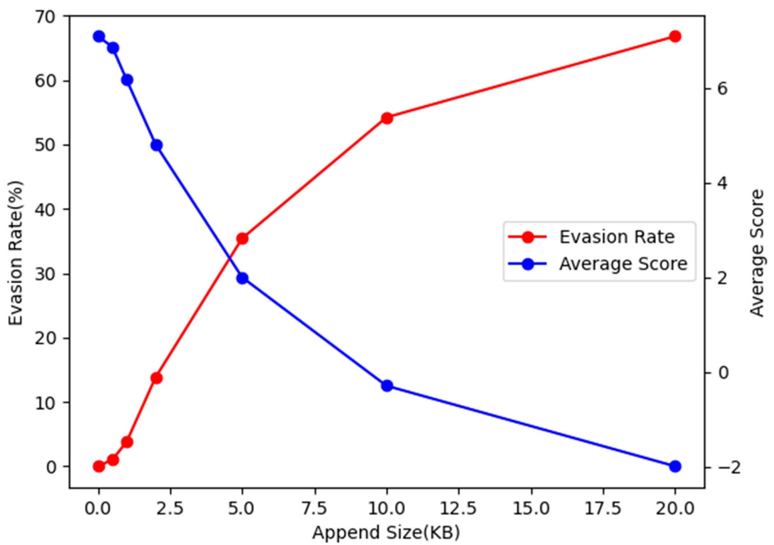
We conduct experiments with perturbation sizes of 0.5 KB, 1 KB, 2 KB, 5 KB, 10 KB, and 20 KB, and record the evasion rate as well as the average confidence score of the generated adversarial examples on the detection model (these confidence scores are not disclosed to the generative model, they are only used for result analysis). The experimental results are shown in Table 1 and Figure 4.
It can be seen from the figure that the evasion rate increases with the increase of the appended size, and the average confidence score decreases accordingly. The rising or falling trends of the two are basically the same, and they are gradually slowing down. This shows that as the appended size grows, the perturbation per KB is less effective. When the appended size reaches the maximum value of 20 KB set in our experiment, 66.8% of the adversarial examples successfully evade the target detection model, which can pose a certain threat to the target detection model as a black-box method.

4.4.2. Iterative Generation Method

The iterative generation method adopts the strategy of generating small perturbations multiple times. In our experiments, we use the RNN generative model to generate an adversarial perturbation with a fixed size of 1 KB each time and attach this perturbation to malicious samples. Then, we query the confidence score of the Malconv model for the current malicious sample and decide whether to keep this adversarial perturbation according to the difference between the confidence scores before and after adding this perturbation. Here, we set the threshold of the confidence score difference as 0.2, i.e., only adversarial perturbations that successfully reduce the confidence score by more than 0.2 will be retained. In addition, we made some restrictions in the experiment. The upper limit of the number of times to query the confidence score of the Malconv model is set to 50, and the upper limit of the total size of the adversarial perturbation is set to 20 KB. Our iterative generation method consumes the number of queries to optimize each adversarial perturbation until an adversarial example that can evade the detection model is successfully generated. If the number of queries or the size of the perturbation reaches the upper limit before then, the generation fails.
Under these conditions, 454 adversarial examples were successfully generated, and the evasion rate reached 90.8%. We counted the distribution of the number of queries and perturbation sizes required to successfully generate adversarial examples, as shown in Figure 5.
It can be seen that the number of queries is mostly distributed within 1–20 times. The append size is mostly concentrated in 1–10 KB, and the peak value is around 3 KB. To reduce the influence of the size of the malicious sample itself on the perturbation scale, we also counted the relative ratio (%) of the perturbation scale and the malicious sample itself. It can be seen that the vast majority of perturbations only account for less than 10% of the original malicious samples, and those with an append size percentage of less than 5% account for more than 60% of all samples.
According to our statistics, among all the samples that successfully generate adversarial examples, the average number of queries is 13.87, the average size of the perturbation is 5541 bytes, and the average ratio of the perturbation size to the original sample size is 6.16%.
Since the evasion rate is affected by two factors, the number of queries and the appended size, we also counted and studied how the evasion rate is affected by these two factors, as shown in Figure 6 and Figure 7.
From the comprehensive analysis and comparison of Figure 6 and Figure 7, it can be seen that both the number of queries and the appended size have a significant marginal effect on the evasion rate. That is to say, with the improvement of these two abilities, the effect on the increase of evasion rate is getting weaker and weaker. Roughly speaking, when the number of queries reaches 30, increasing the number of queries has little effect on improving the evasion rate. Similarly, for the appended size, the improvement of the evasion rate is significantly weakened by adding the appended size after reaching 10 KB or 10% of the original sample size. In addition, the number of queries and the appended size will also interact with each other on the evasion rate results. Due to the settings of our method, each iteration of the query will generate at most 1 KB of adversarial perturbation. When the upper limit of the number of queries is much smaller than the upper limit of the perturbation size (KB), the generated adversarial perturbation will not reach the upper limit of the perturbation size, that is, the full ability of appending perturbation will not be exerted, and vice versa. Therefore, according to the experimental data and our experience, when the number of queries is about 3–4 times of the appended size (KB), better results can be obtained under the current conditions. Moreover, when the two increase simultaneously, the effect of increasing the evasion rate is more obvious, and the effect of improving a certain ability alone is limited.
In conclusion, our iterative generation method can achieve a 90.8% evasion rate under the maximum capacity condition we set (20 KB perturbation, 50 queries). Even if the ability is reduced by about half (10 KB perturbation, 20 queries), the evasion rate of 70.6% can still be achieved. Although each query needs to obtain the confidence score result given by the detection model, compared with the one-time generation method, the iterative method can more accurately find out the adversarial perturbation and can obtain a better evasion rate result at the lowest possible cost.

4.4.3. Comparison with Other Methods

We also compared it with other attack methods that employ the append strategies. We choose two white-box methods and two black-box methods to compare with our method.
  • Benign Features Append (BFA): It is a white box method proposed by Chen et al. [35], which introduces the Grad-CAM method proposed by Selvaraju et al. [45] to generate a saliency vector for the sample. A saliency vector, which contains features of a series of data blocks in an input binary file, can roughly show the benign and malicious regions of the file. Based on the saliency vector, they continuously select data blocks with benign features as perturbations to append to the end of the sample until the detection model is successfully evaded.
  • Enhanced BFA: It is an improved version of the BFA method. This method [35] uses the important benign feature data blocks obtained from the BFA method as the initial perturbation of the FGSM method, which can more efficiently and quickly attract the attention of the model to obtain the backpropagation gradient. Compared with BFA method, it can significantly improve the success rate of evasion.
  • Random Append: It is a relatively simple black-box adversarial method, which appends randomly generated perturbation bytes at the end of the sample to try to evade the detection model.
  • Experience Based Method: It is a black box method proposed by Chen et al. [35]. This method first divides the benign sample into several data blocks and randomly appends the data blocks to the end of the malicious sample until the detection model is successfully evaded. Then, these attacks are repeated, and the contribution of each data block is calculated based on the trajectory of the successful attack. This contribution information replaces the saliency vector in the BFA method, and the subsequent attack process is the same as the BFA method.
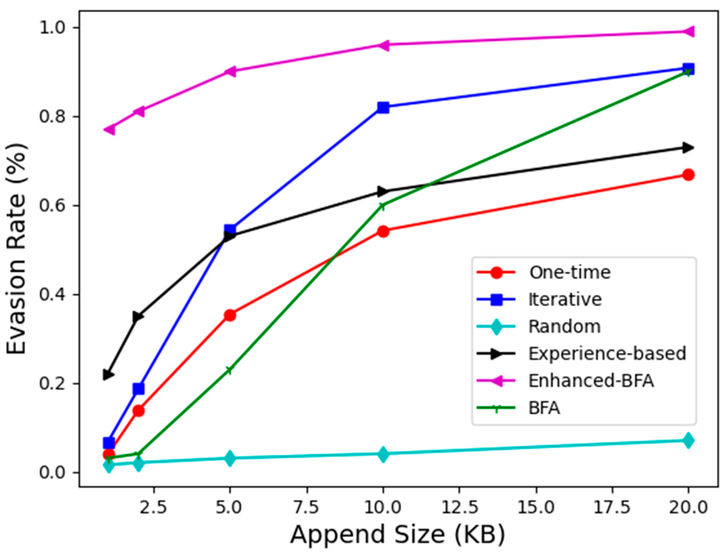
Figure 8 shows the comparison results of evasion rates of several methods under different perturbation scales. First, our method achieves an evasion rate much higher than that of the random append method at any append size, indicating that the adversarial perturbation bytes generated by our method are targeted and the effect is relatively ideal. Furthermore, for the one-time generation method, it tends to vary with the perturbation size roughly the same as the experience-based method, but the evasion rate is slightly lower than that of the experience-based method. For the iterative generation method, when the perturbation size is less than 5 KB, its evasion rate is not as good as that of the experience-based method, but its evasion rate increases rapidly with the increase of the perturbation size. After it is greater than 5 KB, it has surpassed all other black-box methods, and gradually approaches the best white-box method in the figure, the enhanced BFA.
In short, the one-time generation method is a basic method to directly use the RNN generation model to generate adversarial perturbation. The method is relatively simple and direct, and the information required is relatively small. Its evasion rate increases relatively steadily with the change in the perturbation scale. For the iterative generation method, since the perturbation size of our iteration is set to 1 KB, it is difficult to take advantage of iteration when the perturbation size is small (less than 5 KB), and the evasion rate at this time is not high. However, as the perturbation size grows, the evasion rate increases rapidly, surpassing the experience-based black-box method and gradually approaching the enhanced BFA white-box method.

5. Conclusions and Future Work

In this paper, we investigate the problem of insufficient robustness of current end-to-end malware detection models based on deep learning, especially the Malconv model. In recent years, these models, which do not require feature engineering and expert knowledge, are increasingly being used in automated anti-malware systems. Our research shows that under the condition of only obtaining the scores of some benign sample from the detection model, adversaries can train RNN generation models based on this information to generate adversarial perturbations, thereby making adversarial examples on a large scale. This is our one-time generation method, which achieves the highest evasion rate of 66.8%. If the score of the model on the intermediate samples can be obtained during the generation, the scale of additional perturbations can be further reduced and the success rate of evasion can be improved, that is, the iterative generation method, which achieves a maximum evasion rate of 90.8%. These results prove the vulnerability of the current deep learning-based malware detection model. Anti-malware systems usually do not pay enough attention to the detection and scoring information of benign samples, which may give adversaries an opportunity.
In the future, in terms of attack direction, due to the generality of our method, we will consider extending it to other models of the same type. While for other types of models, such as non-end-to-end, based on opcodes or other features, we still consider treating them as sequences and further transfer our method. In the direction of defense, we will consider the most basic adversarial training to improve the robustness of the model. Furthermore, in the introduction to the benign payload, we plot the model confidence score versus the first n bytes of the sample (Figure 2). Our research may imply that models with a smoother and less abrupt curve are more robust and harder to attack. In the future, we may start from this point to study how to improve the defense ability of detection models against adversarial attacks.

Author Contributions

Conceptualization, S.W.; Methodology, S.W.; Software, S.W.; Formal analysis, S.W.; Data curation, S.W. and Z.K.; Writing—original draft, S.W.; Writing—review & editing, S.W., Y.W. and Z.K.; Supervision, J.X. and Y.W.; Project administration, J.X. and Y.W.; Funding acquisition, J.X. All authors have read and agreed to the published version of the manuscript.

Funding

This research and the APC was funded by Major Scientific and Technological Innovation Projects of Shandong Province (2020CXGC010116), the National Natural Science Foundation of China (No. 62172042), and the National Key Research & Development Program of China (2020YFB1712104).

Data Availability Statement

Previously published articles were used to support this study and these prior studies and datasets are cited at relevant places within this article. The link to the datasets is https://virusshare.com/ (accessed on 26 March 2022).

Conflicts of Interest

The authors declare that there is no conflict of interest regarding the publication of this paper.

References

  1. Szegedy, C.; Zaremba, W.; Sutskever, I.; Bruna, J.; Erhan, D.; Goodfellow, I.; Fergus, R. Intriguing properties of neural networks. In Proceedings of the International Conference on Learning Representations (ICLR), Banff, AB, Canada, 14–16 April 2014. [Google Scholar]
  2. Raff, E.; Barker, J.; Sylvester, J.; Brandon, R.; Catanzaro, B.; Nicholas, C. Malware detection by eating a whole EXE. In Proceedings of the 32nd AAAI Workshops, New Orleans, LA, USA, 2–3 February 2018; pp. 268–276. [Google Scholar]
  3. Pietrek, M. Peering Inside the PE: A Tour of the win32 (R) Portable Executable File Format. Microsoft Syst. J. 1994, 9, 15–38. [Google Scholar]
  4. Nataraj, L.; Karthikeyan, S.; Jacob, G.; Manjunath, B. Malware images: Visualization and automatic classification. In Proceedings of the 8th International Symposium on Visualization for Cyber Security, Pittsburgh, PA, USA, 20 July 2011; pp. 1–7. [Google Scholar] [CrossRef]
  5. Simonyan, K.; Zisserman, A. Very deep convolutional networks for large-scale image recognition. arXiv 2014, arXiv:1409.1556. [Google Scholar]
  6. Kaiming, H.; Xiangyu, Z.; Shaoqing, R.; Jian, S. Deep Residual Learning for Image Recognition. In Proceedings of the 2016 IEEE Conference on Computer Vision and Pattern Recognition (CVPR), Las Vegas, NV, USA, 27–30 June 2016; pp. 770–778. [Google Scholar] [CrossRef]
  7. Szegedy, C.; Vanhoucke, V.; Ioffe, S.; Shlens, J.; Wojna, Z. Rethinking the inception architecture for computer vision. In Proceedings of the IEEE Conference on Computer Vision and Pattern Recognition, Las Vegas, NV, USA, 27–30 June 2016; pp. 2818–2826. [Google Scholar]
  8. Hassen, M.; Chan, P. Scalable Function Call Graph-based Malware Classification. In Proceedings of the Seventh ACM Conference on Data and Application Security and Privacy(CODASPY), Scottsdale, AZ, USA, 22–24 March 2017; ACM: New York, NY, USA, 2017; pp. 239–248. [Google Scholar] [CrossRef]
  9. Kinable, J.; Kostakis, O. Malware classification based on call graph clustering. J. Comput. Virol. 2011, 7, 233–245. [Google Scholar] [CrossRef]
  10. Kong, D.; Yan, G. Discriminant malware distance learning on structural information for automated malware classification. In Proceedings of the 19th ACM SIGKDD International Conference on Knowledge Discovery and Data Mining, Chicago, IL, USA, 11–14 August 2013; pp. 1357–1365. [Google Scholar] [CrossRef]
  11. Yan, J.; Yan, G.; Jin, D. Classifying malware represented as control flow graphs using deep graph convolutional neural network. In Proceedings of the 2019 49th Annual IEEE/IFIP International Conference on Dependable Systems and Networks (DSN), Portland, OR, USA, 24–27 June 2019; pp. 52–63. [Google Scholar] [CrossRef]
  12. Santos, I.; Brezo, F.; Ugarte-Pedrero, X.; Bringas, P.G. Opcode sequences as representation of executables for data-mining-based unknown malware detection. Inf. Sci. 2013, 231, 64–82. [Google Scholar] [CrossRef]
  13. Awad, Y.; Nassar, M.; Safa, H. Modeling malware as a language. In Proceedings of the 2018 IEEE International Conference on Communications (ICC), Kansas City, MO, USA, 20–24 May 2018; pp. 1–6. [Google Scholar] [CrossRef]
  14. Jain, S.; Meena, Y.K. Byte level n–gram analysis for malware detection. In Proceedings of the International Conference on Information Processing, Shanghai, China, 13–17 November 2011; Springer: Berlin/Heidelberg, Germany, 2011; pp. 51–59. [Google Scholar] [CrossRef]
  15. Raff, E.; Sylvester, J.; Nicholas, C. Learning the pe header, malware detection with minimal domain knowledge. In Proceedings of the 10th ACM Workshop on Artificial Intelligence and Security, Dallas, TX, USA, 3 November 2017; pp. 121–132. [Google Scholar] [CrossRef]
  16. Goodfellow, I.; Shlens, J.; Szegedy, C. Explaining and harnessing adversarial examples. arXiv 2014, arXiv:1412.6572. [Google Scholar]
  17. Papernot, N.; McDaniel, P.; Goodfellow, I.; Jha, S.; Celik, Z.; Swami, A. Practical Black-Box Attacks against Machine Learning. In Proceedings of the 2017 ACM on Asia Conference on Computer and Communications Security (ASIACCS ′17), Abu Dhabi, United Arab Emirates, 2–6 April 2017; Association for Computing Machinery: New York, NY, USA, 2017; pp. 506–519. [Google Scholar] [CrossRef]
  18. Xu, W.; Qi, Y.; Evans, D. Automatically evading classifiers. In Proceedings of the 2016 Network and Distributed Systems Security Symposium, San Diego, CA, USA, 21–24 February 2016; p. 10. [Google Scholar]
  19. Su, J.; Vargas, D.V.; Sakurai, K. One Pixel Attack for Fooling Deep Neural Networks. IEEE Trans. Evol. Comput. 2019, 23, 828–841. [Google Scholar] [CrossRef]
  20. Kreuk, F.; Barak, A.; Aviv-Reuven, S.; Baruch, M.; Pinkas, B.; Keshet, J. Deceiving end-to-end deep learning malware detectors using adversarial examples. arXiv 2018, arXiv:1802.04528. [Google Scholar]
  21. Kolosnjaji, B.; Demontis, A.; Biggio, B.; Maiorca, D.; Giacinto, G.; Eckert, C.; Roli, F. Adversarial malware binaries: Evading deep learning for malware detection in executables. In Proceedings of the 26th European Signal Processing Conference (EUSIPCO), Rome, Italy, 3–7 September 2018; pp. 533–537. [Google Scholar] [CrossRef]
  22. Demetrio, L.; Biggio, B.; Lagorio, G.; Roli, F.; Armando, A. Explaining vulnerabilities of deep learning to adversarial malware binaries. arXiv 2019, arXiv:1901.03583. [Google Scholar]
  23. Hu, W.; Tan, Y. Generating Adversarial Malware Examples for Black-Box Attacks Based on GAN. In DMBD 2022: Data Mining and Big Data; Communications in Computer and Information Science; Springer: Singapore, 2023; Volume 1745. [Google Scholar] [CrossRef]
  24. Rosenberg, I.; Shabtai, A.; Rokach, L.; Elovici, Y. Generic black-box end-to-end attack against state of the art API call based malware classifiers. In Research in Attacks, Intrusions, and Defenses, Proceedings of the 21st International Symposium, RAID 2018, Heraklion, Crete, Greece, 10–12 September 2018; Proceedings 21; Springer International Publishing: Berlin/Heidelberg, Germany, 2018; pp. 490–510. [Google Scholar] [CrossRef]
  25. Castro, R.L.; Schmitt, C.; Dreo, G. AIMED: Evolving Malware with Genetic Programming to Evade Detection. In Proceedings of the 18th IEEE International Conference on Trust, Security and Privacy in Computing and Communications/13th IEEE International Conference on Big Data Science and Engineering (TrustCom/BigDataSE), Rotorua, New Zealand, 5–8 August 2019; pp. 240–247. [Google Scholar] [CrossRef]
  26. Castro, R.L.; Schmitt, C.; Rodosek, G.D. ARMED: How Automatic Malware Modifications Can Evade Static Detection. In Proceedings of the 5th International Conference on Information Management (ICIM), Cambridge, UK, 24–27 March 2019; pp. 20–27. [Google Scholar] [CrossRef]
  27. Demetrio, L.; Biggio, B.; Lagorio, G.; Roli, F.; Armando, A. Functionality-Preserving Black-Box Optimization of Adversarial Windows Malware. IEEE Trans. Inf. Forensics Secur. 2021, 16, 3469–3478. [Google Scholar] [CrossRef]
  28. Anderson, H.S.; Kharkar, A.; Filar, B.; Evans, D.; Roth, P. Learning to evade static PE machine learning malware models via reinforcement learning. arXiv 2018, arXiv:1801.08917. [Google Scholar]
  29. Chen, J.; Jiang, J.; Li, R.; Dou, Y. Generating Adversarial Examples for Static PE Malware Detector Based on Deep Reinforcement Learning. J. Phys. Conf. Ser. 2020, 1575, 012011. [Google Scholar] [CrossRef]
  30. Song, W.; Li, X.; Afroz, S.; Garg, D.; Kuznetsov, D.; Yin, H. Mab-malware: A reinforcement learning framework for attacking static malware classifiers. arXiv 2020, arXiv:2003.03100. [Google Scholar]
  31. Li, X.; Li, Q. An IRL-based malware adversarial generation method to evade anti-malware engines. Comput. Secur. 2020, 104, 102118. [Google Scholar] [CrossRef]
  32. Anderson, H.S.; Kharkar, A.; Filar, B.; Roth, P. Evading machine learning malware detection. In Proceedings of the Black Hat, Las Vegas, NV, USA, 22–27 July 2017. [Google Scholar]
  33. Park, D.; Khan, H.; Yener, B. Generation and Evaluation of Adversarial Examples for Malware Obfuscation. In Proceedings of the 18th IEEE International Conference on Machine Learning and Applications (ICMLA), Boca Raton, FL, USA, 16–19 December 2019; pp. 1283–1290. [Google Scholar] [CrossRef]
  34. Ebrahimi, M.; Zhang, N.; Hu, J.; Raza, M.T.; Chen, H. Binary black-box evasion attacks against deep learning-based static malware detectors with adversarial byte-level language model. arXiv 2020, arXiv:2012.07994. [Google Scholar]
  35. Chen, B.-C.; Ren, Z.-R.; Yu, C.; Hussain, I.; Liu, J.-T. Adversarial Examples for CNN-Based Malware Detectors. IEEE Access 2019, 7, 54360–54371. [Google Scholar] [CrossRef]
  36. Takase, S.; Suzuki, J.; Nagata, M. Character n-Gram Embeddings to Improve RNN Language Models. Proc. Conf. AAAI Artif. Intell. 2019, 33, 5074–5082. [Google Scholar] [CrossRef]
  37. Kolosnjaji, B.; Zarras, A.; Webster, G.; Eckert, C. Deep Learning for Classification of Malware System Call Sequences. In AI 2016: Advances in Artificial Intelligence; Kang, B., Bai, Q., Eds.; AI 2016. Lecture Notes in Computer Science; Springer: Cham, Switzerland, 2016; Volume 9992. [Google Scholar] [CrossRef]
  38. Rosenberg, I.; Shabtai, A.; Elovici, Y.; Rokach, L. Defense methods against adversarial examples for recurrent neural networks. arXiv 2019, arXiv:1901.09963. [Google Scholar]
  39. Harun Babu, R.; Vinayakumar, R.; Soman, K.P. RNNSecureNet: Recurrent neural networks for Cyber security use-cases. arXiv 2019, arXiv:1901.04281. [Google Scholar]
  40. Zuo, F.; Li, X.; Young, P.; Luo, L. Neural machine translation inspired binary code similarity comparison beyond function pairs. arXiv 2018, arXiv:1808.04706. [Google Scholar]
  41. Cho, K.; Van Merriënboer, B.; Gulcehre, C.; Bahdanau, D.; Bougares, F.; Schwenk, H.; Bengio, Y. Learning phrase representations using RNN encoder-decoder for statistical machine translation. arXiv 2014, arXiv:1406.1078. [Google Scholar]
  42. Chung, J.; Gulcehre, C.; Cho, K.H.; Bengio, Y. Empirical evaluation of gated recurrent neural networks on sequence modeling. arXiv 2014, arXiv:1412.3555. [Google Scholar]
  43. Available online: https://virusshare.com/ (accessed on 26 March 2022).
  44. Available online: https://pytorch.org/ (accessed on 20 March 2022).
  45. Selvaraju, R.R.; Cogswell, M.; Das, A.; Vedantam, R.; Parikh, D.; Batra, D. Grad-cam: Visual explanations from deep networks via gradient-based localization. In Proceedings of the IEEE International Conference on Computer Vision (ICCV), Venice, Italy, 22–29 October 2017; pp. 618–626. [Google Scholar]
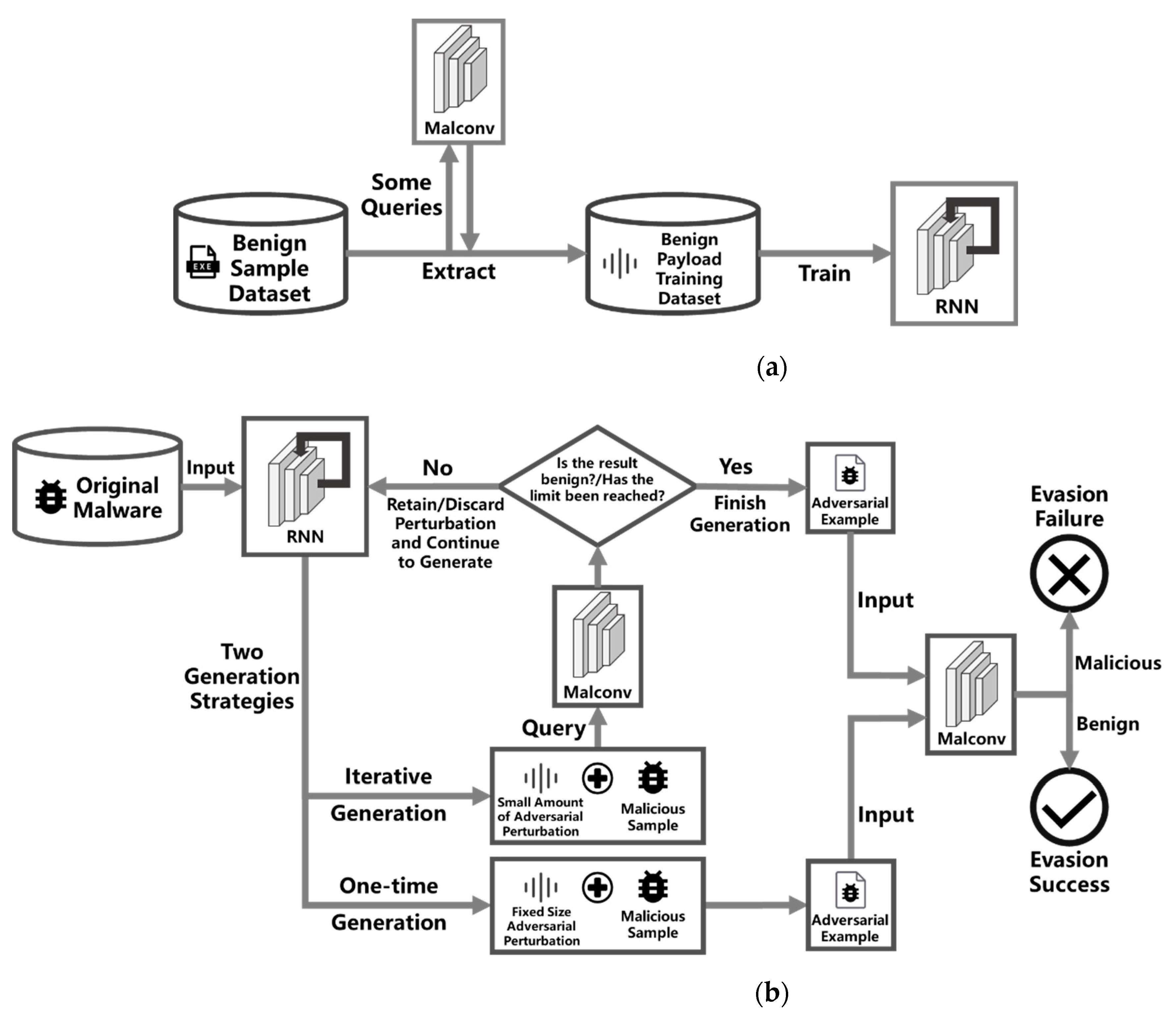
Figure 1. The overall processing flow chart of our method. (a) Flow of RNN generation model training; (b) flow of two adversarial example generation methods.
Electronics 12 02346 g001
Figure 2. Two typical examples of sudden changes (in blue circle) in sample confidence scores for Malconv models.
Electronics 12 02346 g002
Figure 3. Extract training data from sequences of benign samples.
Electronics 12 02346 g003
Figure 4. Evasion rate and average confidence score as a function of append size (KB) using the one-time generation method.
Electronics 12 02346 g004
Figure 5. The distribution of conditions required to successfully generate adversarial examples. (a) The distribution of query times; (b) The distribution of perturbation sizes (KB); (c) The distribution of perturbation sizes (relative ratio).
Electronics 12 02346 g005
Figure 6. (a) Evasion rates under different append sizes (KB) and query times; (b) Evasion rates under different append percent (%) and query times.
Electronics 12 02346 g006
Figure 7. (a) Changes of evasion rate with query times under different append sizes (KB); (b) Changes of evasion rate with query times under different append percent (%); (c) Changes of evasion rate with append size (KB) under different query times; (d) Changes of evasion rate with append percent (%) under different query times.
Electronics 12 02346 g007
Figure 8. The evasion rate of each method under different append sizes.
Electronics 12 02346 g008
Table 1. Results of the one-time generation method at different perturbation sizes.
Perturbation Size/KB00.51251020
Evasion Rate/1.0%3.8%13.8%35.4%54.2%66.8%
Mean Confidence Score7.096.876.174.812.00−0.29−1.99
Disclaimer/Publisher’s Note: The statements, opinions and data contained in all publications are solely those of the individual author(s) and contributor(s) and not of MDPI and/or the editor(s). MDPI and/or the editor(s) disclaim responsibility for any injury to people or property resulting from any ideas, methods, instructions or products referred to in the content.