Article

Soft Segmentation and Reconstruction of Tree Crown from Laser Scanning Data

Institute of Computing Technology, China Academy of Railway Sciences Corporation Limited, Beijing 100081, China
*
Author to whom correspondence should be addressed.
Electronics 2023, 12(10), 2300; https://doi.org/10.3390/electronics12102300
Submission received: 28 April 2023 / Revised: 14 May 2023 / Accepted: 17 May 2023 / Published: 19 May 2023
(This article belongs to the Section Computer Science & Engineering)

Abstract

:
Point cloud data obtained by laser scanning can be used for object shape modeling and analysis, including forest inventory. One of the inventory tasks is individual tree extraction and measurement. However, individual tree segmentation, especially tree crown segmentation, is challenging. In this paper, we present a novel soft segmentation algorithm to segment tree crowns in point clouds automatically and reconstruct the tree crown surface from the segmented crown point cloud. The soft segmentation algorithm mainly processes the overlapping region of the tree crown. The experimental results showed that the segmented crown was accurate, and the reconstructed crown looked natural. The reconstruction algorithm was highly efficient in calculating the time and memory cost aspects since the number of the extracted boundary points was small. With the reconstructed crown geometry, the crown attributes, including the width, height, superficial area, projecting ground area, and volume, could be estimated. The algorithm presented here is effective for tree crown segmentation.

1. Introduction

The forest is closely related to human life and is an essential element of the metaverse and other virtual spaces, including three-dimensional (3D) computer games and movies. Whether studying forestry or modeling geometrical tree shapes, it is necessary to obtain forest data. A convenient and efficient way to obtain forest data is to use remote sensing technology, such as terrestrial fixed-point or airborne LiDAR, to scan a forest. These kind of data consist of a large number of discrete points in 3D space, called point clouds. In point cloud data, each point is recorded as 3D coordinates ( x , y , z ) . Compared to 2D image data, it has accurate three-dimensional position information without scaling or deformation. As pointed out in previous studies, the successful detection and delineation of individual trees from forest point cloud is critical, allowing for studies of individual tree demography, growth modeling, and more precise measures of biomass [1]. However, the segmentation of an individual tree, especially tree crown segmentation, is not easy. Apart from the coordinates of the points, we should estimate other information, such as the connection relationship and neighborhood relationship of these points.
As for the individual trees and the crown segmentation from LiDAR data, many methods have been presented in the past ten years. These existing methods can be roughly divided into three categories.
The first category method is based on treetop detection. When the tree spacing at the upper lever is large, exploiting the spacing between the tops of trees is effective to identify and group points into a single individual tree [2]. After a treetop has been detected, the tree climbing method can be applied to identify the individual tree, and then a donut expanding and sliding method tree can be used to detect the crown boundary and isolate the individual trees [3]. Another way is that after the treetop has been detected, it is consecutively connected and accumulated by vertically traversing the point layers, which results in the individual tree delineation [4]. The canopy height model can be used for coarse segmentation, and the segmented results can be refined using a multi-direction 3D profile analysis and K-mean clustering [5]. In addition, tree segmentation can be practiced by combining the local maxima (treetop) with the growing region algorithm or Voronoi tessellation method. However, in some cases, these combination methods do not provide better results than the tree relative distance algorithm [6].
The second category is based on horizontally cut clusters. A representative method is layer stacking, which slices the entire forest point cloud at 1-m height intervals and isolates the trees in each layer. Then, merging the results from all the layers produces the representative tree profiles [7]. A simpler method than layer stacking is the projection algorithm, which projects the point cloud onto the xOy plane and employs the hybrid clustering technique, including a combination of DBSCAN and K-means, to segment the individual trees from the forest point cloud [8]. It has been observed that the point density decreases with an increasing distance from the trajectory. A distance-dependent algorithm that considers the inhomogeneities in point density was developed for the segmentation of the forest point clouds [9]. To overcome the limitation of the method that takes the highest point in a filtering window as the tree position, H. Liu et al. used the cluster center of the higher points to detect the tree position [10].
The third category method is based on the fusion of multiple algorithms. Given the complexity of forest point cloud segmentation, a processing chain consisting of the stand delineation, canopy height model, characterization, and point clustering with an adaptive mean shift was proposed [11]. For terrestrial backpack LiDAR data, the individual trees were extracted based on DBSCAN clustering and a cylinder voxelization of the volume, which showed a high detection rate for the tree locations [12]. To improve the results of the individual tree detection algorithms, M. Lisiewicz et al. proposed a three-step approach to correct the segmentation errors [13]. Recently, the structure and geometry shape were considered for improving the segmentation effect. For example, for individual tree crown segmentation from laser data that focuses on overstory and understory trees, a framework that combines the detection of the symmetrical structure of the trees and mean shift clustering was proposed [14]. With branch–trunk constraints, a hierarchical clustering method was proposed to extract street trees from mobile laser scanning (MLS) point clouds [15]. Using the shape of the scanline and circle fitting, an individual tree can be segmented, and the stem attributes can be estimated [16]. In addition, the application of a convolutional neural network to perform the tree crown detection and delineation has also been developed [17].
The reconstruction of a tree and a tree crown is a direct follow-up to point cloud segmentation, which measures tree properties more accurately and conveniently. The reconstructed geometrical models also show reality and can be used in virtual scenes in the virtual community, 3D computer games, movies, etc. In the past decades, much literature has proposed methods for reconstructing trees and tree crowns. Here, we only investigate some of the typical existing methods published in recent years.
Most of the reconstruction algorithms consist of the following four steps: (i) the segmentation of a TLS tree point cloud separating the wooden parts from foliage, (ii) the reconstruction of the trunk and branches, (iii) the distribution of the foliage within the tree crown using the points of the foliage cloud as the attractors, and (iv) the generation of a 3D representation [18]. The points from the leaves and branches can be segmented based on the convergence of the local principal curvature directions and the region growing method [19]. The tree trunk and branch geometries and topological structures are constructed based on skeleton extraction and then fitted with cylinders [20,21]. Therefore, the structural analysis and optimization of the extracted skeleton are often emphasized [22].
Tree crown segmentation and reconstruction is one of the key points in tree segmentation, which has received more and more attention. Although terrestrial laser scan point clouds can provide precise feature observation of vegetation architecture and improve agricultural monitoring and management [23], the incompleteness that stems from the branch or leaf occlusion impairs the detection accuracy of the tree attributes. Reconstructing the tree crown geometry from the point clouds can compensate for this incompleteness for a better tree attribute estimation.
For the tree crown reconstruction, the crown points should be detected first from the point cloud. The distribution of the foliage within the tree crown uses the points of the foliage cloud as the attractors [18]. Paris et al. [24] presented a data fusion approach to extract the crown structures by exploiting the complementary perspective of airborne laser scanning. Cici et al. [25] delineated the tree crowns from the airborne laser scanning data using a Delaunay triangulation. The early crown reconstruction methods mainly employ surface fitting with a cylinder or paraboloid fitting surfaces [26]. Kato et al. [27] used radial basis functions (RBFs) to reconstruct the implicit surfaces approximating the individual tree crown shapes, and the tree crown formation was captured through the implicit surface reconstruction [28]. Lin et al. [29] provided a new method by combining the mobile mapping mode and a multi-echo-recording laser scanner to enhance the integrity of the individual tree crown reconstruction.
The other typical methods for reconstructing the tree crown geometry include the α -shape method [30], the region-based level set method [31], and a voxel-based method to add leaves to a reconstructed 3D branch structure [32].
The direct surface fitting method for the crown surface reconstruction is short on details, and current other methods have a relatively high time cost for the computation. However, in some cases, the time efficiency of the reconstruction algorithm must be considered. For example, in vehicle [33] and airborne [34] laser scanning, the fast reconstruction of objects is very important for real-time monitoring and analyzing the scene [9,35]. The existing experiment results showed that crown segmentation in a multi-layered closed canopy forest could be improved using 3D segmentation methods rather than primarily relying on the canopy surface model [36].
The above methods were effective for tree counting and single tree separation. However, most of the methods did not pay attention to the crown shape, especially the overlapping of adjacent tree crowns, causing the shape and size of the crown to be overlooked and the shape reconstruction effect to lack realism. The former is essential for forest inventory, and the latter is important for digital model construction.
In this paper, we propose a new tree crown segmentation and reconstruction method based on terrestrial laser scan point clouds to obtain accurate tree crown segmented point clouds and their realistic geometrical reconstruction. Furthermore, our method can enhance the visual effects of reconstructed crowns with improved surface shape accuracy and enhance the reconstruction process.
The main highlights of this work include the following.
(1)
Construct an algorithm for segmenting and reconstructing tree crowns from laser scanning data, which can be applied to the forest inventory.
(2)
Propose a soft segmentation algorithm for making the reconstructed tree crown more natural and accurate.
(3)
Propose a fast reconstruction algorithm that fuses down-sampling and constructs a kd-tree.
The rest of this article is organized as follows. Section 2 describes the data we used and the proposed method in detail. Section 3 discusses the experimental results and the analysis for evaluating the proposed method. In the last section, Section 4, we conclude and list several limitations.

2. Data and Methods

Figure 1 illustrates the overview of our method’s framework. The input data consisted of a raw point cloud. Only 3D coordinates of all the points were used. After segmenting the crown points from the branch points using the principal curvature direction distribution method, the proposed soft segmentation algorithm was used to obtain the individual tree points. Then, the 3D silhouette surface was reconstructed. Finally, the tree geometry and the other attributes were estimated using the reconstructed trees.

2.1. Data

The point cloud of the two pine trees used in our experiment was captured using a Cyrax or RIGEL scanner on the Peking University campus. The number of points in each scan was approximately 269,366 and 487,555, respectively. Each point was represented by 3D coordinates (x, y, z). The length (unit: meter) in directions x, y, and z were 8.47/11.19/11.12 and 10.19/9.31/11.94 in the two scans, respectively. The information is listed in detail under the tree images, as shown in Figure 2.
For testing the proposed soft segmentation algorithm, we combined two point clouds (Figure 2a,b) to form a large point cloud (Figure 2c). The experimental purpose of combining two trees at different intervals for segmentation was twofold. Firstly, it was done to obtain the simulated data of the overlapping tree crowns. On the other hand, it was used to study whether the accuracy of the proposed method was affected by the two trees with different degrees of overlap.
The second set of experimental data was street trees extracted from the Oakland point cloud data (Figure 3a). The Oakland point cloud data were collected around the Carnegie Mellon University (CMU) campus in Oakland, using Navlab11 equipped with side looking SICK LMS laser scanners, and were opened by D. Munoz et al. [37]. The distance between two adjacent trees on the roadside was manually planned, and the distance between them was relatively large. Most of the adjacent trees had no intersecting areas between their crowns, resulting in accurate individual trees isolated using most of the existing methods, such as region growth or clustering. Therefore, we only chose two trees with overlapping crowns, as shown in Figure 3b, and named OaklandTrees to test our proposed soft segmentation algorithm.
Another set of experimental data was three pair of trees, which were extracted from RUSH07, as shown in Figure 4a. The point cloud data were acquired in the native Eucalypt open forest (dry sclerophyll box-ironbark forest) [38] in Victoria, Australia. Please refer to the introduction of this database for the geographic information and the data composition of the scanned plot.
Three pair of trees were selected as the experimental data because our main interest was in the segmentation of trees with overlapping crowns. The data, RUSH07, was segmented into several groups, and there were no overlapping areas between the tree crowns of the groups. Although there were more than three pair of groups with overlapping tree crowns, the three selected pairs, named RUSH07treesA, RUSH07treesB, and RUSH07treesC, as shown in Figure 4b–d, respectively, were representative. The difficulty of segmenting the three pair of trees was different. RUSH07treesA consisted of two trees with the same height. RUSH07treesB displayed an interlocking phenomenon between adjacent tree crowns. RUSH07treesC was composed of two trees with different heights, which were relatively close together. The information about those three pair of trees can be found in Figure 4b–d.

2.2. Soft Segmentation

The proposed soft segmentation (SoftSeg) algorithm mainly deals with the crown points from two adjacent trees. SoftSeg consists of four steps: the crown points extraction; the crown layers partition; the vertical partition; and the layer contour extraction and refinement.

2.2.1. Crown Points Extraction

This step segments the crown points Ω C from the trunk and branch points Ω B in the point cloud Ω , which consists of two trees, as shown in Figure 2c, for example.
Ω = Ω C Ω B
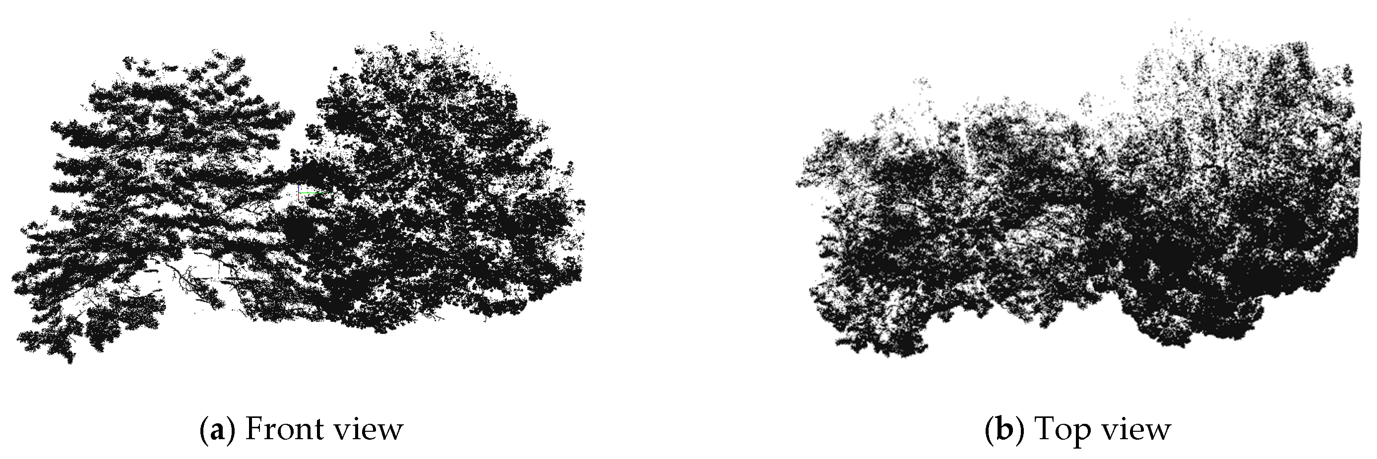
The segmentation algorithm for the branch and leaf separation can be any one of the existing approaches. We employed the principal curvature direction-based method proposed in the literature [19]. Based on the key assumption that the neighbor points from the branches usually have similar principal directions and the neighbor points from the leaves do not have this feature, the curvature direction-based algorithm consists of several steps. However, the first three steps can be used to the separate trunk and branch points from the leaf points. The first step is to estimate the principal directions and the principal curvatures of each point. The second step is to build the axis distribution of each point. The last step is to discriminate the point from a branch or a leaf by employing a threshold. Figure 5 shows the segmented crown points from Figure 2c.
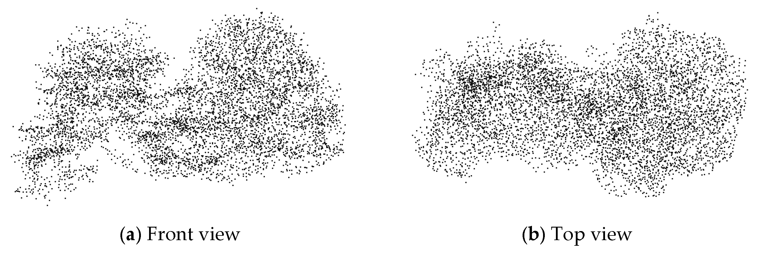
As shown in Figure 5b, the top view of the segmented crown highlights the density of the point cloud in different regions of the extracted crown. The non-uniformity of the point cloud was potentially caused by unilateral laser scanning and self-occlusion, resulting in an unstable distance threshold value when the 3D surface was reconstructed.
We used the down-sampling method to overcome the influence of the non-uniformity of the point cloud density, similar to the voxel-based method [32]. Then, the sparse and uniform crown part points Ω C ( s ) were obtained from Ω C . Figure 6a (6176 points) shows the s down-sample visual effect from Figure 5a (708,504 points).
In this way, the number of sampling points was dramatically reduced. Only 0.872% of the points were used for the crown segmentation and reconstruction. The shape of the tree crown point cloud after down-sampling was, in general, consistent with its original figure.

2.2.2. Vertical Partition

According to the segmentation results of the branch and leaf point cloud (Section 2.2.1), the tree roots ( C 1 and C 2 ) and the trunk top positions were detected. Therefore, we used the minimum cut plane to construct the coarse segmentation of the two tree point clouds. The approach consisted of three steps: partitioning the points into slices, finding the optimal dividing line, and obtaining the initial segmentation of the point cloud.
The first step was to partition points into slices. Assuming that the thickness v b of each slice was 0.2 m, then the number of slices was the quotient obtained by dividing the distance between C 1 and C 2 by v b , as shown in Formula (2).
N v b = C 1 C 2 v b
Figure 7 illustrates the method for generating slices along the line C 1 to C 2 . Note that the partition was performed in 3D space, and the local coordinate system [ C 1 ; C 1 C 2 o , C 1 Y , C 1 Z ] was not the same as that of the laser scanner, where only the direction of the z-axis was the same. C 1 C 2 o is a unit vector parallel to C 1 C 2 . Let C 1 ( x c , y c , z c ) , then any point p i x i , y i , z i belongs to the i t h slice B i , if i = ( x i x c ) 2 + ( y i y c ) 2 v b . In this way, all the points in Ω C ( s ) were partitioned into m slices.
The second step was to find the optimal dividing line, which was defined by the minimum cut plane and could be obtained using the solution of the minimum–maximum optimal problem, as shown in Formula (3).
i * = arg min i max j z j p j ( z j , z j , z j ) B i }
The last step was to segment the points into three categories: the unlabeled set, the point set from the first tree, and the point set from the second tree, labeled as 0, 1, and 2, respectively.
The label L ( p i ) of a point p i x i , y i , z i was determined by a partitioning rule. If p i B j , then
L p i = 0 , o t h e r w i s e 1 , j < i * ε 2 , j > i * + ε
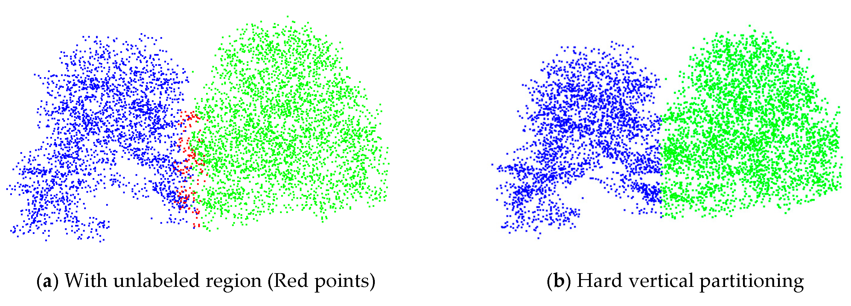
where ε N , known as the overlap width, is a parameter specified by the user and related to the overlap level of two crowns. The vertical partition result is shown in Figure 6a, where ε = 1 . If the unlabeled case is deleted, Formula (4) is transformed into the following.
l p i = 1 , j i * 2 , j > i *
Formula (5) defines a kind of hard vertical partitioning, known as the hard segmentation method (HS), which segments the point cloud (Figure 6) into Figure 8b. From the subfigure, it can be found that after segmenting, the shape between the two segmented crowns was a straight line, which is generally not a natural shape since the adjacent tree crowns often overlap.
To improve the visual effect of the crown shape, Formula (4) was employed in our soft segmentation algorithm. The point in the intersection region was classified into the unlabeled point set, which was processed in the following subsections.

2.2.3. Crown Layers Partition

Unlike the methods that project 3D points on the ground or use an x O y plane to achieve the biggest crown contour, we used a method similar to the layer stacking method [7]. In this way, the shape of each layer of the crown contour was tighter.
For the crown point set Ω C ( s ) , the layer bins δ i ( i = 1,2 , , k ) were generated from horizontal slices. Figure 9 shows the partitioning effect.
Let k be the number of bins.
Ω C ( s ) = δ 1 δ 2 δ k
The cutting was uniform in the upward direction, and the thickness b of each bin was calculated using Formula (7).
b = 1 k ( Z m a x Z m i n )
where Z m a x = max z P ( x , y , z ) Ω C ( s ) } and Z m i n = min z P ( x , y , z ) Ω C ( s ) } . The number of bins k is a parameter whose value depends on the laser scanning resolution. If the value of k is appropriate, each bin δ i is neither too thick nor too thin. In our experiment, the thickness b of each bin was set to approx. 0.5 m, and the parameter k = 20, specified according to the experiment data that the height of the trees used in our experiments were approx. 10 m. In this way, all the points were partitioned into these bins.

2.2.4. Layer Contour Extraction and Refinement

The unlabeled points in the intersection region were processed, as shown in Figure 10. This problem was similar to recovering the missing part of the crown. By referring to an idea that repairs the missing points based on their shape and structure [39], we also fully used the point cloud contour and optimized the shape of each layer bin.
The contour of each layer bin was extracted by projecting the points in the bin onto the horizontal cross-section in the middle of the bin and employing the two-dimensional (2D) contour extraction algorithm. The 2D contour was obtained sequentially, connecting the farthest projection point in each direction. For example, as shown in Figure 10, the farthest projection point in angle A 1 O A 2 was A 1 . The number of directions ( m = 9, 18 or 36) was specified by the experimental test.
Using the 2D contour extraction approach, we obtained the contour of each layer tree by tree, L p i = 1 or 2, as shown in Figure 11a. Figure 11c provides an example of a layer where the contours of the two trees did not overlap, and the unlabeled (red) points were not determined as to which tree they belonged to.
For an unlabeled point p , L p = 0 , we inferred its new label, according to the contour shape, distance, and randomized assignment. We first calculated d 1 and d 2 , which were the distances from p to the contours of Tree 1 and Tree 2, respectively. Then we used the Monte Carlo method to label p as one or two, according to the probability.
P l a b e l = e d 2 / d 1
The idea behind this formula was that the farther away from the contour of one tree, the lower the probability of belonging to this tree. Figure 11b,d show the effect of the updated segmentation and the refined contour.
Since our algorithm included a random classification strategy for the overlap region points, its effect achieved the simulation of the intersection of the crown contour. The algorithm was called the soft segmentation (SoftSeg) algorithm.

2.3. Reconstruction

After the terrestrial laser scan point clouds have been soft segmented, the points of a tree are taken as the input for crown surface reconstruction. The input data, denoted as Ω, include N points, and each point Pi(i = 1, 2, …, N) were represented only by its position coordinates (x, y, z), without regard to other information that laser scanners may generate besides the position coordinates. The direction of the z-axis is upward, which will guide the horizontal cutting of our method.
After inputting the laser scan point cloud of a tree, we first segment crown points (denoted as C) out from branches, then reconstruct the crown as following steps.

2.3.1. Detecting Boundary Points of Bins

For each layer bin, the boundary points were detected based on a 2D α-shape. The classical α-shape method was introduced by H. Edelsbrunner in 1983 [40], and Bernardini et al. [41] improved it to probe the boundary of a point set by setting α = r 2 , in which r is the radius of a disc in a 2D plane or a ball in 3D space. In our case, we projected all the points of a bin onto a horizontal plane xOy, as shown in Figure 10, and obtained the boundary points of each original bin based on Bernardini’s method [41].

2.3.2. Building the Crown Surface

After obtaining the boundary points of each bin, the crown surface geometry was constructed based on a 3D α -shape [42]. Let Λ be the set of all the boundary points Q j (j = 1, 2, …, n b ) of the crown. We constructed a kd-tree data structure [43] on Λ to speed up the procedure of constructing the surface. The Algorithm 1 known as the “Building Crown Surface with Boundary Points” (or BCSwBPs) was given in pseudocode as follows.
Algorithm 1: BCSwBPs.
Input: Λ , α
 Output: crown surface geometry
 S1: construct a kd-tree with all points in the set Λ
 S2: for Q i , Q j , Q k Λ
 S3: calculate two centers C 1 , C 2 of two balls B 1 , B 2 . Note that Q i , Q j , Q k are on B m and C m Q n = α , m = 1 , 2 ; n = i , j , k .
 S4: Find a nearest neighbor Q d 1 of C 1
 S5: Find a nearest neighbor Q d 2 of C 2
 S6: if Q d 1 B 1 or Q d 2 B 2 , then
 S7:   Δ Q i Q j Q k is a boundary triangle for output
 S8: end if
 S9: end for

2.3.3. Estimating the Attributes

With the reconstructed crown surface, several crown attributes, including the width, height, superficial area, and projecting ground area, were estimated.
The width W c r o w n of a tree crown was estimated according to Formula (9).
W c r o w n = max { P i P j ¯ , P i , P j Γ }
where Γ is the boundary of the projection points set that vertically mapped Λ onto the xOy plane.
The height H c r o w n of the crown was estimated using the laser scanning point data.
H c r o w n = Z m a x Z m i n
where Z m a x and Z m i n are the maximum and minimum z-coordinates of the crown.
The superficial area of the crown was the sum of the areas of all the triangles on the surface of the crown. In the traditional α -shape method, the triangles in the crown were turned into boundary triangles if the radius r of the probing ball was too small. This led to a bigger superficial area than the real case. If the r was set too large, the reconstructed crown would become a convex hull, which would also induce a significant error. As our method only used the boundary points to build the crown surface, the superficial area only consisted of the boundary triangles, making the error small.
For calculating the projecting ground area, all the points of Λ were projected onto the xOy plane, and a polygon P was built on these projected points by employing a 2D α -shape method. Note that the polygon P may not always be convex, and the built P based on projecting C or Λ onto the xOy plane is the same.
For calculating the reconstructed tree crown volume, the geometrical information of each layer bin could be used again. The volume was estimated using Formula (11).
V t r e e = 1 3 b i = 0 k 1 ( S i + S i + 1 + S i S i + 1 )
where S i is the cross-sectional area of the i t h layer bin.

3. Results

We demonstrated the effectiveness of the SoftSeg and BCSwBPs algorithms based on the point cloud segmentation and reconstruction experiments. Our algorithm was written in C++ language with the support of OpenGL for visualization. The experiments were conducted on a laptop with an Intel(R) Core(TM) i7-4710MQ [email protected] and a 4 GB RAM.

3.1. Segmentation of the Tree Crown with Different Overlap Degrees

A pair of trees composed of the same two trees, if their distances are different, means that the degree of overlap between tree crowns is also different. The experiment was to test the segmentation effect of the point cloud from two trees at different distances. As shown in the first column of Figure 12, the distance between two tree roots was 6.464, 6.962, 7.46, 7.959, 8.457, 8.956, and 9.455 m, respectively. These seven point clouds were segmented using our SoftSeg algorithm, and the result of each step is displayed in Figure 12. It can be found that the overlap region was classified in the view of the crown shape, which showed a realistic silhouette.
For quantitatively evaluating the effect of the segmentation of our method, we computed the accuracy (Ac) and precision (Pre) and compared our results to those from the hard segmentation (Formula (5)).
The accuracy was calculated using Formula (12).
A c = ( m 11 + m 22 ) / N
The sensitivity was calculated using Formula (13).
P r e = m 11 / ( m 11 + m 21 )
where m 11 is the number of points correctly classified to Tree 1; m 22 is the number of points correctly classified to Tree 2; m 21 is the number of points wrongly classified to Tree 1; and N is the total number of points of the input data.
We compared the results obtained by the proposed soft segmentation method (SS, or SoftSeg) to the results obtained by the hard segmentation method (HS, Formula (5) in Section 2.2.2). The quantitative results are listed in Table 1. In the table, the number of points in Tree 1 and Tree 2 were 3253 and 2923, respectively.
As for the symbols in the table in the first column (series number, SN) of the table, Rowi ( i = 1 , 2 , , 7 ) consisted of the point cloud data from the i t h row in Figure 12. Tru.T1 is the number of points that belongs to Tree 1. HS.T1 means that those points are classified into Tree 1 using the hard segmentation method. HS.T1p is the ratio of HS.T1 to the number of points from Tree 1. “SS” is the abbreviation of “SoftSeg”. Similarly, we defined the other symbols, including HS.T2, HS.T2p, SS.T1, SS.T1p, SS.T2, and SS.T2p.
Using the data listed in Table 1 and with Formulas (12) and (13), the values of the Ac and Pre were calculated and are displayed in Figure 13. From the line charts, we can conclude that as the overlapping area of the two trees decreased, the accuracy of segmentation continued to increase. Both line charts showed that compared to the HS algorithm, the SS algorithm improved slightly in both the accuracy and precision. Due to the small proportion of the points in the overlapping part of the crown of the two trees to the total number of points, the segmentation accuracy and precision seemed to improve only slightly. However, in view of the sum of misclassification points in Table 1, the misclassification rate of the SS is approx. 4% lower than that of the HS.

3.2. Segmentation and Comparison

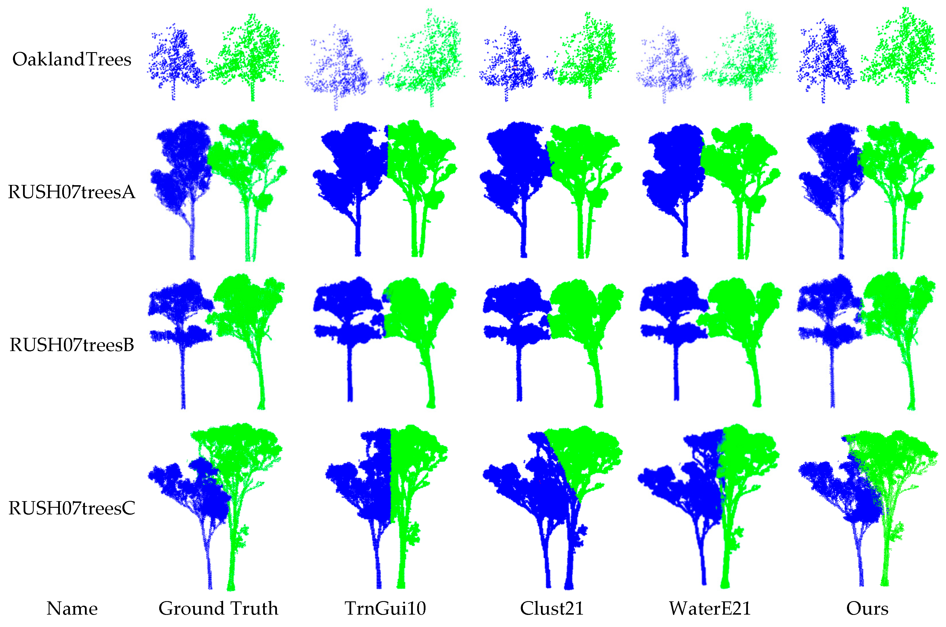
Four pair of trees, OaklandTrees (Figure 3b), RUSH07treesA (Figure 4b), RUSH07treesB (Figure 4c), and RUSH07treesC (Figure 4d), were used for testing the performance of our proposed method (SoftSeg).
The experimental results of our method were compared to those of three representative methods: trunk guided crown segmentation (TrnGui10) [44], DBSCAN-based clustering (Clust21) [8], and the water expansion method (WaterE21) [45]. The segmentation results of the four point clouds after down-sampling are shown in Figure 14.
By comparing the segmented results to the ground truth (the second column in Figure 14), it can be found that when there was an apparent valley between the adjacent trees, WaterE21 showed the best performance in the view of the visual effect. Our method achieved the best performance among the four listed methods when RUSH07treesC was segmented.
For the quantitative comparison, the confusion matrixes of the four pair of trees segmented using the four methods are listed in Table 2. In the table, “Pts.N” means the number of points of the corresponding point cloud data. The bold confusion matrixes achieved the best results among the four methods. This table showed that both the WaterE21 and our methods achieved the best segmentation results since the diagonal elements in their confusion matrix were relatively large.
According to the confusion matrixes and Formula (11), the accuracy (Ac) of the segmentation results could be calculated. The values of the segmentation accuracy of the four pair point clouds segmented using the four methods are displayed as line chart in Figure 15. From the perspective of the segmentation accuracy, these four segmentation methods accurately segmented the three point cloud data, OaklandTrees, RUSH07treesA, and RUSH07treesB, and the segmentation accuracies were all greater than 90%. However, for the segmentation of RUSH07treesC, only our method had a segmentation accuracy exceeding 90%, showing an optimal robustness.
The average accuracies of the four segmentation results were 91.79%, 94.00%, 95.05%, and 97.06%, obtained by the four methods, TrnGui10, Clust21, WaterE21, and ours, respectively. This means that in the experiment of segmenting these four point cloud data, our algorithm achieved the best performance.

3.3. Reconstruction Results

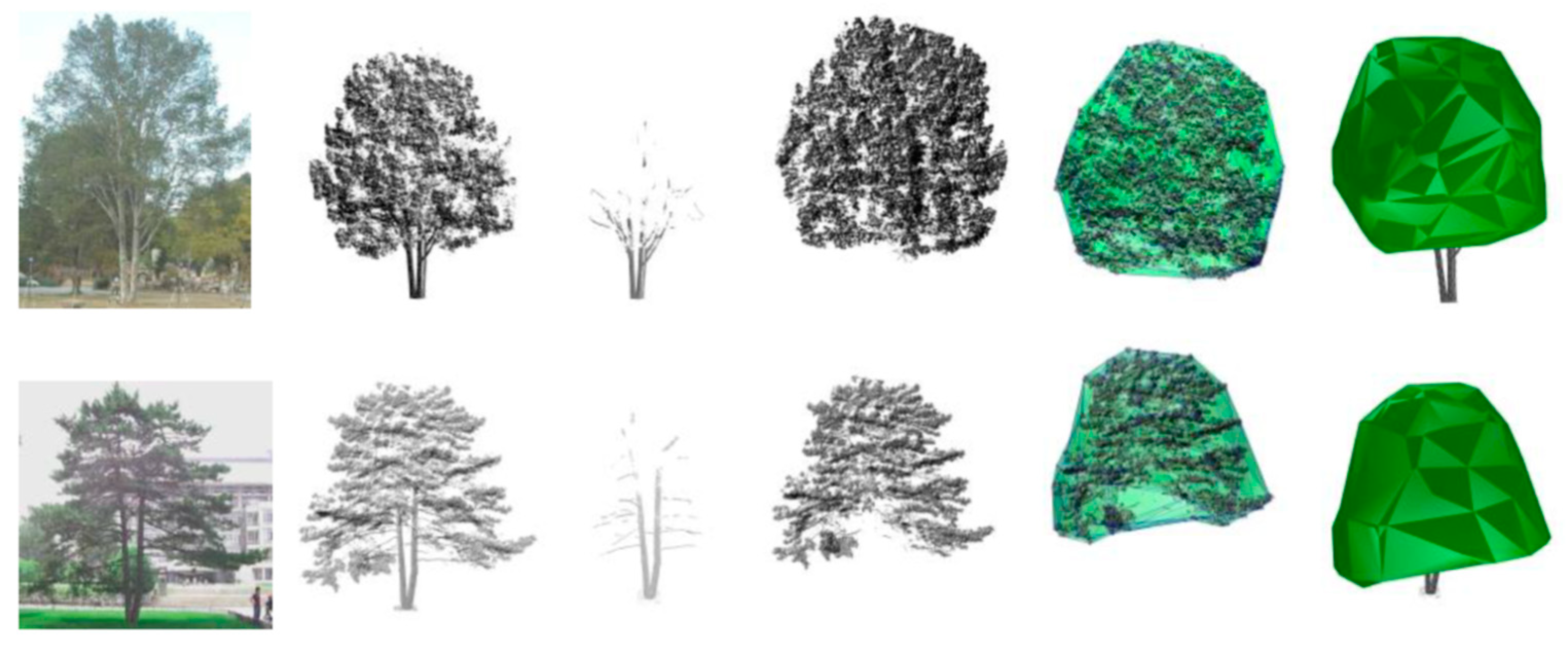
For the two pine trees, we used our method to construct each tree crown, respectively, as shown in Figure 16.
The related attributes are listed in Table 3, with ”SN” denoting the serial number of the tree, “N.Pts” the number of scanning points, “H.Tree” the height (m) of the tree, “W.Tree” the width (m) of the tree, “A.Sup” the superficial area (m2) of the reconstructed crown, and “A.proj” the projection area (m2) of the reconstructed crown.
For the point cloud, Oaklandtrees (Figure 3), after the segmentation with our SoftSeg method, all the tree shape silhouette meshes were reconstructed, as illustrated in Figure 17. The attributes of all the trees are listed in Table 4. In this table, the volume was calculated using Formula (11), and its unit was m3. As shown in Table 4, the point cloud of each segmented tree was very sparse, and the accuracy of the calculated attribute values needs further verification in future research.
For the three point clouds of the three pair of trees, as shown in Figure 4, after the segmentation using the SoftSeg method, the reconstructed mesh models of the individual trees are displayed in Figure 18. To enhance the visual differentiation, the different pair trees models used different colors. Visually, these silhouette mesh models have a more natural appearance.

3.4. Discussion

3.4.1. Time Efficiency with Down-Sampling

A down-sampling step was employed to improve the time efficiency of the individual tree segmentation processing. The time (seconds) of the segmentation of RUSH07TreesA is recorded in Table 5. In the table, “DS” means the down-sampling step. From the table, we can safely conclude that the down-sampling step significantly improved the algorithm efficiency because the time cost of the method without the DS step was approx. 28 times of the efficiency with the DS step.

3.4.2. Error Caused by Down-Sampling

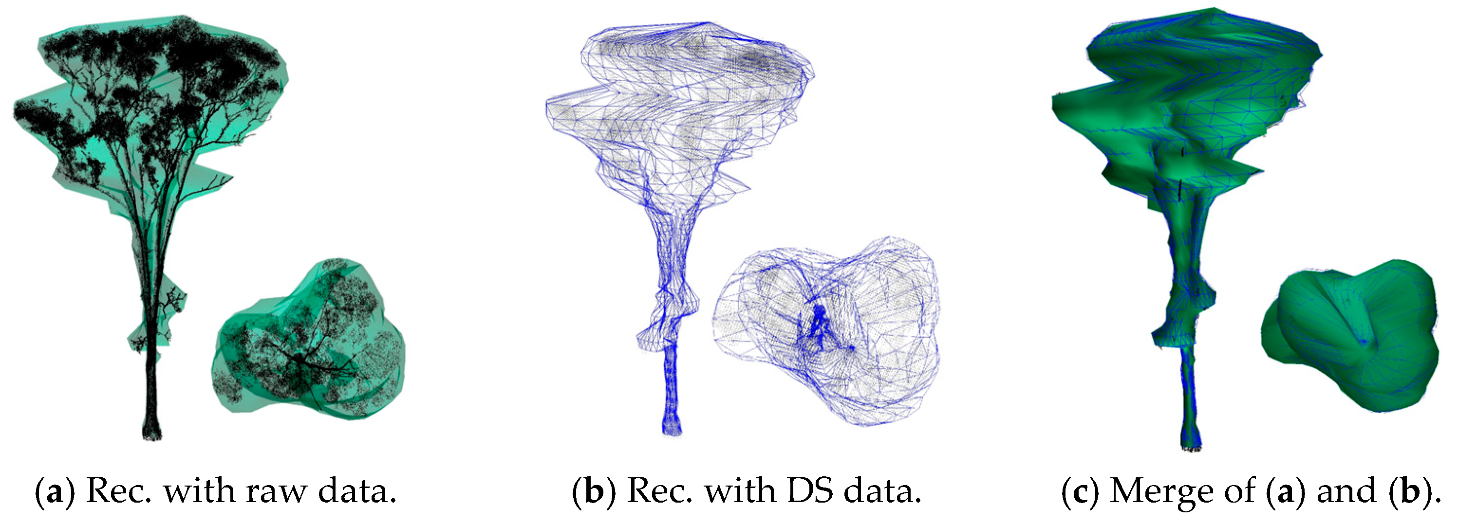
As for the implications of down-sampling, it is possible to cause minor errors when the attributes, including the volume and surface area of the tree crowns, are estimated. However, the impact of down-sampling on the silhouette shape of the tree crowns is relatively tiny. We used one tree extracted from RUSH07TreesC to check the implications. In this experiment, the layer number k was set to 38 (different from the value used in Figure 18), about 0.5 m thick. The reconstructed silhouette surface mesh is illustrated in Figure 19. The reconstructed mesh consisted of 1369 vertices and 2700 triangles. The average length of the triangle edge was 0.8481 m, and the average area of all the triangles was 0.202 m 2 .
With the reconstructed shape, the attributes were estimated and are listed in Table 6. The table shows that the relative error was very small (less than 1.6%), even though the number of the model points was compressed by 93%. Therefore, the down-sampling step can be introduced into the algorithm process to improve the algorithm efficiency.

3.4.3. Visual Effect of the Reconstructed Crown

In addition, the proposed SoftSeg method had an advantage over the hard segmentation methods, for example, TrnGui10 [44], in that the visual effect of the crown shape that was reconstructed using the point cloud segmented by SoftSeg was often better than that of the hard segmentation method. Figure 20 illustrates the visual effect by comparing our method to the reconstructed crown from the segmented point cloud using TrnGui10 method. The points were ground truth. The purple silhouette surface was the reconstructed tree shape. Obviously, the hard segmentation method often caused the vertical segmentation plane, decreasing the visual reality.

3.4.4. Segmentation Using the Deep Learning Method

We did not consider deep learning methods as a comparative method but rather part of the discussion. This was primarily because we did not have enough labeled data for the training set. We adopted the Pointnet++ [46] to segment the trees. The test set consisted of one point cloud in Figure 12 and four point clouds in Figure 14. The training set consisted of six point clouds in Figure 12 and one point cloud in Figure 14. After setting the parameters, batch_size = 2, decay_rate = 0.0001, epoch = 20, learning_rate = 0.001, lr_decay = 0.5, optimizer = ‘Adam’, step_size = 20, the line charted the training accuracy, the test accuracy, and the class average mIOU in the training and the testing processes are displayed in Figure 21. The last test accuracy was approx. 90.0%, which was far less than the segmentation accuracy of our method. However, with the establishment of labeled datasets for forest segmentation in the future, deep learning methods will provide excellent performance.

4. Conclusions

In this paper, we proposed a novel tree crown soft segmentation algorithm called SoftSeg, which was automatic if the number of layer bins and the overlap width was assigned as the default values. The experiments showed that the new algorithm could effectively segment the different overlapping degrees of the crown of two trees. Compared to hard segmentation, it could improve the segmentation accuracy, over 90%, and reduce the misclassification point. The crown silhouette shape reconstructed from the points segmented by SoftSeg was more realistic than that obtained using the hard segmentation method. In addition, to improve the algorithm efficiency, two strategies, down-sampling and kd-tree, were used in the proposed method. In practical applications, if it was necessary to study the distribution characteristics of the branches and leaves in the overlapping area of the tree crowns, the proposed method could be an alternative solution.
Our algorithm had several limitations. First, the reconstructed mesh quality should be given more attention, which could be improved by employing an existing mesh optimal algorithm. Second, when the point cloud was severely missing, down-sampling could not supplement enough missing information, so the reconstructed crown shape was also incomplete. Solving the reconstruction of the severely missing point cloud data could also be a challenging task. Another limitation was that the segmentation results had apparent errors, and further improvement is needed in the future.

Author Contributions

Conceptualization, M.D.; methodology, M.D. and G.L.; software, M.D.; validation, M.D.; formal analysis, M.D.; investigation, M.D.; resources, M.D. and G.L.; data curation, M.D.; writing—original draft preparation, M.D.; writing—review and editing, M.D. and G.L.; visualization, M.D.; supervision, G.L.; project administration, G.L.; funding acquisition, M.D. and G.L. All authors have read and agreed to the published version of the manuscript.

Funding

This research received no external funding. This research was funded by the China Academy of Railway Sciences Corporation Limited, grant number 2021YJ197.

Data Availability Statement

The first author can provide point clouds of two pine trees, please send an email to get in contact; for RUSH07, please refer to TERN, https://portal.tern.org.au/metadata/23868, accessed on 1 March 2023; for OaklandTrees, please visit http://www.cs.cmu.edu/~vmr/datasets/oakland_3d/cvpr09/doc/, accessed on 18 May 2023.

Conflicts of Interest

The authors declare no conflict of interest.

References

  1. Jakubowski, M.K.; Li, W.; Guo, Q.; Kelly, M. Delineating Individual Trees from LiDAR Data: A Comparison of Vector- and Raster-based Segmentation Approaches. Remote Sens. 2013, 5, 4163–4186. [Google Scholar] [CrossRef]
  2. Li, W.; Guo, Q.; Jakubowski, M.K.; Kelly, M. A New Method for Segmenting Individual Trees from the Lidar Point Cloud. Photogramm. Eng. Remote Sens. 2012, 78, 75–84. [Google Scholar] [CrossRef]
  3. Zhang, C.; Zhou, Y.; Qiu, F. Individual Tree Segmentation from LiDAR Point Clouds for Urban Forest Inventory. Remote Sens. 2015, 7, 7892–7913. [Google Scholar] [CrossRef]
  4. Wang, J.; Lindenbergh, R.; Menenti, M. Scalable individual tree delineation in 3D point clouds. Photogramm. Rec. 2018, 33, 315–340. [Google Scholar] [CrossRef]
  5. Yang, J.; Kang, Z.; Cheng, S.; Yang, Z.; Akwensi, P.H. An Individual Tree Segmentation Method Based on Watershed Algorithm and Three-Dimensional Spatial Distribution Analysis From Airborne LiDAR Point Clouds. IEEE J. Sel. Top. Appl. Earth Obs. Remote Sens. 2020, 13, 1055–1067. [Google Scholar] [CrossRef]
  6. Irlan, I.; Saleh, M.B.; Prasetyo, L.B.; Setiawan, Y. Evaluation of Tree Detection and Segmentation Algorithms in Peat Swamp Forest Based on LiDAR Point Clouds Data. J. Manaj. Hutan Trop. J. Trop. For. Manag. 2020, 26, 123–132. [Google Scholar] [CrossRef]
  7. Ayrey, E.; Fraver, S.; Kershaw, J.A., Jr.; Kenefic, L.S.; Hayes, D.; Weiskittel, A.R.; Roth, B.E. Layer Stacking: A Novel Algorithm for Individual Forest Tree Segmentation from LiDAR Point Clouds. Can. J. Remote Sens. 2017, 43, 16–27. [Google Scholar] [CrossRef]
  8. Chen, Q.; Wang, X.; Hang, M.; Li, J. Research on the improvement of single tree segmentation algorithm based on airborne LiDAR point cloud. Open Geosci. 2021, 13, 705–716. [Google Scholar] [CrossRef]
  9. Bienert, A.; Georgi, L.; Kunz, M.; von Oheimb, G.; Maas, H.-G. Automatic extraction and meas-urement of individual trees from mobile laser scanning point clouds of forests. Ann. Bot. 2021, 128, 787–804. [Google Scholar] [CrossRef]
  10. Liu, H.; Dong, P.; Wu, C.; Wang, P.; Fang, M. Individual tree identification using a new clus-ter-based approach with discrete-return airborne LiDAR data. Remote Sens. Environ. 2021, 258, 112382. [Google Scholar] [CrossRef]
  11. Qin, Y.; Ferraz, A.; Mallet, C.; Iovan, C. Individual tree segmentation over large areas using airborne LiDAR point cloud and very high resolution optical imagery. In Proceedings of the 2014 IEEE Geoscience and Remote Sensing Symposium, Quebec City, QC, Canada, 13–18 July 2014; pp. 800–803. [Google Scholar] [CrossRef]
  12. Comesaña-Cebral, L.; Martínez-Sánchez, J.; Lorenzo, H.; Arias, P. Individual Tree Segmentation Method Based on Mobile Backpack LiDAR Point Clouds. Sensors 2021, 21, 6007. [Google Scholar] [CrossRef] [PubMed]
  13. Lisiewicz, M.; Kamińska, A.; Kraszewski, B.; Stereńczak, K. Correcting the Results of CHM-Based Individual Tree Detection Algorithms to Improve Their Accuracy and Reliability. Remote Sens. 2022, 14, 1822. [Google Scholar] [CrossRef]
  14. Huo, L.; Lindberg, E.; Holmgren, J. Towards low vegetation identification: A new method for tree crown segmentation from LiDAR data based on a symmetrical structure detection algorithm (SSD). Remote Sens. Environ. 2022, 270, 112857. [Google Scholar] [CrossRef]
  15. Li, J.; Cheng, X.; Xiao, Z. A branch-trunk-constrained hierarchical clustering method for street trees individual extraction from mobile laser scanning point clouds. Measurement 2021, 189, 110440. [Google Scholar] [CrossRef]
  16. Pires, R.D.P.; Olofsson, K.; Persson, H.J.; Lindberg, E.; Holmgren, J. Individual tree detection and estimation of stem attributes with mobile laser scanning along boreal forest roads. ISPRS J. Photogramm. Remote Sens. 2022, 187, 211–224. [Google Scholar] [CrossRef]
  17. Braga, J.R.G.; Peripato, V.; Dalagnol, R.; Ferreira, M.P.; Tarabalka, Y.; Aragão, L.E.O.C.; Velho, H.F.d.C.; Shiguemori, E.H.; Wagner, F.H. Tree Crown Delineation Algorithm Based on a Convolutional Neural Network. Remote Sens. 2020, 12, 1288. [Google Scholar] [CrossRef]
  18. Janoutová, R.; Homolová, L.; Novotný, J.; Navrátilová, B.; Pikl, M.; Malenovský, Z. Detailed reconstruction of trees from terrestrial laser scans for remote sensing and radiative transfer modelling applications. Silico Plants 2021, 3, diab026. [Google Scholar] [CrossRef]
  19. Dai, M.; Li, H.; Zhang, X. Tree Modeling through Range Image Segmentation and 3D Shape Analysis. In Lecture Notes in Electrical Engineering Book Series (LNEE)2010; Springer: Berlin/Heidelberg, Germany, 2010; Volume 67, pp. 413–422. [Google Scholar] [CrossRef]
  20. Livny, Y.; Yan, F.; Olson, M.; Chen, B.; Zhang, H.; El-Sana, J. Automatic reconstruction of tree skeletal structures from point clouds. ACM Trans. Graph. 2010, 29, 151:1–151:8. [Google Scholar] [CrossRef]
  21. Zhang, X.; Li, H.; Dai, M.; Ma, W.; Quan, L. Data-driven synthetic modeling of trees. IEEE Trans. Vis. Comput. Graph. 2014, 20, 1214–1226. [Google Scholar] [CrossRef]
  22. Wang, Z.; Zhang, L.; Fang, T.; Mathiopoulos, P.T.; Qu, H.; Chen, D.; Wang, Y. A Structure-Aware Global Optimization Method for Reconstructing 3-D Tree Models From Terrestrial Laser Scanning Data. IEEE Trans. Geosci. Remote Sens. 2014, 52, 5653–5669. [Google Scholar] [CrossRef]
  23. Moorthy, I.; Miller, J.R.; Berni, J.A.J.; Zarco-Tejada, P.; Hu, B.; Chen, J. Field characterization of olive (Olea europaea L.) tree crown architecture using terrestrial laser scanning data. Agric. For. Meteorol. 2011, 151, 204–214. [Google Scholar] [CrossRef]
  24. Paris, C.; Kelbe, D.; van Aardt, J.; Bruzzone, L. A Novel Automatic Method for the Fusion of ALS and TLS LiDAR Data for Robust Assessment of Tree Crown Structure. IEEE Trans. Geosci. Remote Sens. 2017, 55, 3679–3693. [Google Scholar] [CrossRef]
  25. Alexander, C. Delineating tree crowns from airborne laser scanning point cloud data using delaunay triangulation. Int. J. Remote Sens. 2009, 30, 3843–3848. [Google Scholar] [CrossRef]
  26. Morsdorf, F.; Meier, E.; Kötz, B.; Itten, K.I.; Dobbertin, M.; Allgöwer, B. LIDAR-based geometric reconstruction of boreal type forest stands at single tree level for forest and wildland fire management. Remote Sens. Environ. 2004, 92, 353–362. [Google Scholar] [CrossRef]
  27. Kato, A.; Schreuder, G.F.; Calhoun, D.; Schiess, P.; Stuetzle, W. Digital surface model of tree canopy structure from LiDAR data through implicit surface reconstruction. In Proceedings of the ASPRS 2007 Annual Conference, Tampa, FL, USA, 7–11 May 2007. [Google Scholar]
  28. Kato, A.; Moskal, L.M.; Schiess, P.; Swanson, M.E.; Calhoun, D.; Stuetzle, W. Capturing tree crown formation through implicit surface reconstruction using airborne lidar data. Remote Sens. Environ. 2016, 113, 1148–1162. [Google Scholar] [CrossRef]
  29. Lin, Y.; Hyyppa, J. Multiecho-Recording Mobile Laser Scanning for Enhancing Individual Tree Crown Reconstruction. IEEE Trans. Geosci. Remote Sens. 2012, 50, 4323–4332. [Google Scholar] [CrossRef]
  30. Zhu, C.; Zhang, X.; Hu, B.; Jaeger, M. Reconstruction of Tree Crown Shape from Scanned Da-Ta; Springer: Berlin/Heidelberg, Germany, 2008. [Google Scholar]
  31. Tang, S.; Dong, P.; Buckles, B.P. Three-dimensional surface reconstruction of tree canopy from lidar point clouds using a region-based level set method. Int. J. Remote Sens. 2012, 34, 1373–1385. [Google Scholar] [CrossRef]
  32. Xie, D.; Wang, X.; Qi, J.; Chen, Y.; Mu, X.; Zhang, W.; Yan, G. Reconstruction of Single Tree with Leaves Based on Terrestrial LiDAR Point Cloud Data. Remote Sens. 2018, 10, 686. [Google Scholar] [CrossRef]
  33. Kim, D.; Jo, K.; Lee, M.; Sunwoo, M. L-shape model switching-based precise motion tracking of moving vehicles using laser scanners. IEEE Trans. Intell. Transp. Syst. 2017, 19, 598–612. [Google Scholar] [CrossRef]
  34. Ma, Q.; Su, Y.; Tao, S.; Guo, Q. Quantifying individual tree growth and tree competition using bi-temporal airborne laser scanning data: A case study in the Sierra Nevada Mountains, California. Int. J. Digit. Earth 2017, 11, 485–503. [Google Scholar] [CrossRef]
  35. Yu, X.; Hyyppä, J.; Kaartinen, H.; Hyyppa, H.; Maltamo, M.; Rnnholm, P. Measuring the growth of individual trees using multi-temporal airborne laser scanning point clouds. In Proceedings of the ISPRS Workshop on “Laser Scanning 2005”, Enschede, The Netherlands, 12–14 September 2005; pp. 204–208. [Google Scholar]
  36. Aubry-Kientz, M.; Dutrieux, R.; Ferraz, A.; Saatchi, S.; Hamraz, H.; Williams, J.; Coomes, D.; Piboule, A.; Vincent, G. A Comparative Assessment of the Performance of Individual Tree Crowns Delineation Algorithms from ALS Data in Tropical Forests. Remote Sens. 2019, 11, 1086. [Google Scholar] [CrossRef]
  37. Daniel Munoz, J.; Bagnell, A.; Vandapel, N.; Hebert, M. Contextual Classification with Functional Max-Margin Markov Networks. In Proceedings of the IEEE Computer Society Conference on Computer Vision and Pattern Recognition (CVPR), Miami, FL, USA, 20–25 June 2009. [Google Scholar]
  38. Calders, K. Terrestrial Laser Scans—Riegl VZ400, Individual Tree Point Clouds and Cylinder Models, Rushworth Forest; Version 1; Terrestrial Ecosystem Research Network: Indooroopilly, QLD, Australia, 2014. [Google Scholar] [CrossRef]
  39. Fang, H.; Li, H. Counting of Plantation Trees Based on Line Detection of Point Cloud Data; Geomatics and Information Science of Wuhan University: Wuhan, China, 2022; Volume 7. [Google Scholar] [CrossRef]
  40. Edelsbrunner, H.; Kirkpatrick, D.; Seidel, R. On the shape of a set of points in the plane. IEEE Trans. Inf. Theory 1983, 29, 551–559. [Google Scholar] [CrossRef]
  41. Bernardini, F.; Bajaj, C. Sampling and Reconstructing Manifolds Using Alphashapes. 1997. Available online: https://docs.lib.purdue.edu/cgi/viewcontent.cgi?article=2349&context=cstech (accessed on 12 April 2023).
  42. Edelsbrunner, H.; Mücke, E.P. Three-dimensional alpha shapes. ACM Trans. Graph. 1994, 13, 43–72. [Google Scholar] [CrossRef]
  43. Arya, S.; Malamatos, T.; Mount, D.M. Space-time tradeoffs for approximate nearest neighbor searching. J. ACM 2009, 57, 1–54. [Google Scholar] [CrossRef]
  44. Li, H.; Zhang, X.; Jaeger, M.; Constant, T. Segmentation of forest terrain laser scan data. In Proceedings of the 9th ACM SIGGRAPH Conference on Virtual-Reality Continuum and its Applications in Industry (VRCAI ’10), Association for Computing Machinery, New York, NY, USA, 12–13 December 2010; pp. 47–54. [Google Scholar] [CrossRef]
  45. Yun, T.; Jiang, K.; Li, G.; Eichhorn, M.P.; Fan, J.; Liu, F.; Chen, B.; An, F.; Cao, L. Individual tree crown segmentation from airborne LiDAR data using a novel Gaussian filter and energy function minimization-based approach. Remote Sens. Environ. 2021, 256, 112307. [Google Scholar] [CrossRef]
  46. Qi, C.R.; Yi, L.; Su, H.; Guibas, L.J. Pointnet++: Deep hierarchical feature learning on point sets in a metric space. Adv. Neural Inf. Process. Syst. 2017, 30, 1–10. [Google Scholar]
Figure 1. The framework of the proposed method.
Electronics 12 02300 g001
Figure 2. Point cloud data were all scanned on the Peking University campus. The length unit was listed in meters in these experimental data.
Electronics 12 02300 g002
Figure 3. Point cloud data from Oakland [37]. Subfigure (b) shows two trees, named OaklandTrees, labeled with a purple square in Subfigure (a).
Electronics 12 02300 g003
Figure 4. Point cloud data, RUSH07 [38], and the three pair of trees were extracted from RUSH07. (a) RUSH07; (b) RUSH07treesA; (c) RUSH07treesB; and (d) RUSH07treesC.
Electronics 12 02300 g004
Figure 5. The extracted crown shown in two different views.
Electronics 12 02300 g005
Figure 6. The down-sampling result Ω C ( s ) of the extracted crown Ω C .
Electronics 12 02300 g006
Figure 7. Generated slices using vertical partitioning.
Electronics 12 02300 g007
Figure 8. The vertical partitioning of the point cloud.
Electronics 12 02300 g008
Figure 9. The horizontal partitioning of the point cloud.
Electronics 12 02300 g009
Figure 10. The 2D contour extraction of the points.
Electronics 12 02300 g010
Figure 11. The segmentation was refined by partitioning all the unclassified points and optimizing the layer contour.
Electronics 12 02300 g011
Figure 12. The segmentation of two trees pieced together at different distances. From top to bottom, the distance between the two tree roots was 6.464, 6.962, 7.46, 7.959, 8.457, 8.956, and 9.455 m, respectively. From left to right: the input, layer bins, initial segmentation, initial contours of layer bins, refined segmentation, and contours.
Electronics 12 02300 g012
Figure 13. Comparison of the Ac and Pre of the segmentation using the hard segmentation (HS) method and the soft segmentation (SS) method. (a) The accuracy (Ac) of the segment results of the HS and SS methods. (b) The precision (Pre) of the segment results of the HS and SS methods.
Electronics 12 02300 g013
Figure 14. Visual comparison of four pair trees which are segmented using four methods.
Electronics 12 02300 g014
Figure 15. The accuracy (Ac) comparison of the four pair of trees which were segmented using the four methods.
Electronics 12 02300 g015
Figure 16. Crown reconstruction process illustrated with pine trees denoted as Pine 1 and Pine 2. Each row shows the tree crown reconstruction results. The first column is a photo of the tree. The second column is the laser scan point cloud The third points from branches, the fourth the points from the crown, and the fifth shows the reconstructed crown silhouette surface, which was merged with the crown points. The last column shows the reconstructed crown merged with the branch points.
Electronics 12 02300 g016
Figure 17. Crown reconstruction results using the Oakland data.
Electronics 12 02300 g017
Figure 18. The reconstructed tree silhouette mesh model from the point clouds after using the soft segmentation method.
Electronics 12 02300 g018
Figure 19. The reconstructed mesh models used point clouds with/without down-sampling (DS). A subfigure at the bottom right of each figure is the top view of the reconstructed model.
Electronics 12 02300 g019
Figure 20. Visual comparison of the reconstructed tree silhouette mesh models from the point cloud RUSH07TreesC using the TrnGui10 and our SoftSeg methods.
Electronics 12 02300 g020
Figure 21. The training accuracy, the test accuracy, and the class average mIOU varied in the training and testing process.
Electronics 12 02300 g021
Table 1. The confusion matrixes of the hard segmentation and soft segmentation methods. Each matrix was 2 × 2, and the elements on the diagonal of a matrix represent the correct number of segmentation points or the corresponding ratio of points.
SNClassHS.T1HS.T2HS.T1pHS.T2pSS.T1SS.T2SS.T1pSS.T2p
Row1Tru.T130921610.95050.049530781750.94620.0538
Tru.T223826850.08140.918622726960.07770.9223
Row2Tru.T1325030.99910.00093242110.99660.0034
Tru.T236525580.12490.875134125820.11670.8833
Row3Tru.T13253010325120.99940.0006
Tru.T228026430.09580.904227026530.09240.9076
Row4Tru.T13253010325120.99940.0006
Tru.T218027430.06160.938416227610.05540.9446
Row5Tru.T132530103253010
Tru.T228526380.09750.902527926440.09540.9046
Row6Tru.T132530103253010
Tru.T25228710.01780.98224228810.01440.9856
Row7Tru.T132530103253010
Tru.T22229010.00750.99251829050.00620.9938
Table 2. The confusion matrixes of the four pair of trees segmented using the four methods.
NamePts.NTrnGui10Clust21WaterE21Ours
OaklandTrees13701351191319511370013700
8340834083408340834
RUSH07TreesA33,42427,505591929,072435233,27814630,8122612
43,286043,286043,2867643,2102343,263
RUSH07TreesB33,84932,592125733,52432533,849033,709140
27,065027,065127,064727,0584827,017
RUSH07TreesC34,05323,25510,79825,063899022,83111,22230,9063147
24,057210621,951024,05710523,952150622,551
Table 3. Attributes of the two pine trees (Figure 16).
SNN.PtsH.TreeW.TreeA.SupA.proj
Tree1487,55511.910.1292.571.7
Tree2269,36611.111.1303.373.1
Table 4. Attributes of the segmented 17 trees (Figure 17).
Tree SNN.PtsH.TreeW.TreeA.SupVolume
19777.1386.515113.10964.803
24356.7473.33446.00212.153
39786.6546.454108.75648.789
415278.7457.293176.111123.144
513708.6017.687158.965108.512
68347.5405.727112.83554.985
7126710.0647.283185.166121.502
814279.6109.353220.818153.500
913199.0038.101176.291115.188
1010429.8167.222172.671108.886
1110839.1578.454168.591109.401
1213339.5079.000273.591174.541
1310248.8587.363182.16298.426
147777.8805.909112.26949.672
156778.0554.57696.32737.486
168347.4376.111130.31165.083
171224.2651.39413.4991.379
Table 5. The running time (s) of each step of the algorithm for segmenting RUSH07TreesA.
MethodDSRoots
Detect
Layer Bin
Build
Vertical PartitioningContour
Build
Segmentation
Refine
Total
Time
With DS0.0680.34460.01890.01070.01190.00230.4564
Without DS012.40510.24330.15490.26510.021513.0899
Table 6. Attributes of one tree from RUSH07TreesC (Figure 18).
MethodN.PtsN.PolygonH.TreeW.TreeA.SupVolume
With DS34,053270023.17613.333545.831532.967
Without DS536,461270023.31813.412549.142525.064
Error−93.65%0.00%−0.61%−0.59%−0.60%1.51%
Disclaimer/Publisher’s Note: The statements, opinions and data contained in all publications are solely those of the individual author(s) and contributor(s) and not of MDPI and/or the editor(s). MDPI and/or the editor(s) disclaim responsibility for any injury to people or property resulting from any ideas, methods, instructions or products referred to in the content.