Benefits of Monthly Storage Rates in Shared Storage for Energetic Communities ^†

Abstract

Community energy storages, i.e., central battery storages that take over the self-consumption optimisation of energetic communities, can play a central role in the cellular structure of the energy system. However, if the central storage is only used for optimising households’ self-demand, the use is neither economical nor efficient. Therefore, it is conceivable to use the storage for different applications. This article focused on a monthly storage rate for households in energetic communities. First, different households’ storage capacities were determined to demonstrate the benefits of a monthly adjustment in the shared storage for households and storage operators. The advantages are shown compared to annual storage rates and they can be seen on both sides. Households can increase their degree of self-sufficiency and their self-consumption rate through the monthly storage rates. In addition, the storage operator gains more security through the fixed monthly storage rates and has further opportunities to generate revenue through daily sales. In some months, the results show a secondary use potential of over 82% related to the monthly rate, which is determined by the complete data set and additionally substantiated for two exemplary households. In the second part of the article, the annual and monthly storage rates for different kinds of households were transferred into a multiple linear regression model. The model enables us to determine the monthly and annual storage rates of households on the basis of the annual electricity consumption, the installed photovoltaic power, and the rated power of the electric vehicle charging station as well as the heat pump. The estimated results show small deviations from the calculated results and can be used to simplify the planning of the community energy storage for various districts.

1. Introduction

Upcoming energy systems will be predominantly dependent on renewable energy sources at the low and medium voltage levels. To cope with this complex supply task, grid operators intend to increase the balancing of energy supply and demand at the local level [1,2]. Additionally, feed-in tariffs for photovoltaic (PV) systems are decreasing faster than for other renewable energy sources, while the price of electricity for private household (HH) continues to rise due to inflation and ongoing crises [3,4].

Compared to many individual home energy storages (HES), larger community energy storages (CES) that can be accessed by all residents have a number of advantages. For example, the space requirement and the risk of a fire load in the HH are eliminated. In addition, CES offers the chance that an even larger share of self-generated energy can be consumed within the district, as generation and consumption peaks can be more balanced in the community [5,6]. However, if the storage is only used to increase the self-consumption of the HH, the operation of the storage is neither economical nor efficient [7]. Previous studies have shown that an increase in economic efficiency is possible when the storage is used for multiple applications [8,9,10]. The reason for this is that in residential areas with optimised energy use, only $20\%$ of the storage capacity is used to optimise demand throughout the year [5]. Although the multitude of applications in multi-use operation reduces the lifetime of the CES, recent studies demonstrate the increasing cost-effectiveness of the method despite the shorter lifetime [11]. In addition, the much larger CES has a decisive advantage, as the larger surplus units can be marketed in a more targeted manner. Although the potential of storage cannot be fully exploited due to imperfect forecasts of generation and consumption, studies suggest that a significant proportion can be used for grid and system services. This raises the question of what proportion is essential for optimising household self-consumption and what surplus storage is available for a secondary use (SU) of the storage operator.

In addition, a centralised battery storage system raises the question of the necessary size for the energetic community. The issue can be subordinately derived from the necessary storage rate of the different HH in the community. In this work, the question of the storage rate for different time periods (daily, monthly, yearly), as well as a calculation for different types of households, was determined. Of particular interest here are parameters to size CES, allowing the necessary storage rate for a variety of communities to be determined.

1.1. Related Studies

The concept of CES was first introduced by American Electric Power in 2005. Here, CES refers to storages in the range of hundreds of kWh that are located close to households or commercial clients [12]. Already, multiple-use applications have been seen as advantages of CES in addition to single-use applications for end-users [13]. Moreover, various studies deal with the technologies used for CES [14,15] and the economical aspects [16], as well as the design and operation in the energy system [17,18,19]. Especially for the multi-use applications, the authors of [7] give a broad overview of potential services in Germany. They considered the six most promising services to be the direct marketing of power, intraday trading, charging of electric vehicle (EV), peak load shaving, peer-to-peer power trading and energy balancing. The researchers point out that storage’s state of charge (SOC) plays an essential role in the selection of secondary application. There is no analysis of storage shares per month in the context of this work, but the authors point out in a second publication that monthly shares are used [5]. The authors of [20] presented the fundamentals of battery energy storage’s use for the primary control reserve (PCR) provision in Germany. The authors showed the technical requirements for the operation of storage’s as PCR provision systems and provided explanations of the PCR market and regulation. Individual fees are charged for market access on different points. The authors of [21] pointed out that it is important how the CES is connected to the individual houses and where there is a legal entity in the district. However, current research in this area shows that storage operators need to be clear in advance about the size of the storage and therefore the storage rate required by households.

From the customers’ point of view, numerous works focus on the storage rate of HES for optimising the self-consumption of residential load demand and local PV generation profiles. The cost-effectiveness of HES can either be easily determined with the help of online tools [22,23,24,25] or evaluated with comprehensive analyses such as [26] or [27]. Findings show that small home storage systems are profitable for private operation. The authors of [28] proposed limiting the usable storage capacity to a maximum of 1.5 kWh per 1 kW of PV power. Nevertheless, the storage rate is often oversized and too-large storage units are unprofitable, as they are only in demand for few days [28]. Unlike HES, CES are much larger units. This enables storage operators to offer a wide range of economical applications. Conversely, the share of customers will not only be limited to the most economical storage size, but seasonal adjustments will also have to be taken into account. Therefore, the design of HES and CES can be very different and the focus of related studies is limited to CES. However, the research trend shows the need for simple methods to plan the storage rate for the first time.

Furthermore, the comparison between HES and CES has been discussed. The authors of [29] showed that a CES for an urban district has significant efficiency gains compared to distributed storage systems. The specific size of the CES is not specified in the paper, nor are the storage rates of the residents. In their subsequent work [6], the technical advantages of a CES compared to HES were presented. The storage rates per HH were calculated using the average daily consumption of a year. For a district in Cambridge, USA, the authors of [30] demonstrated that CES’s optimal size is only 65% compared to HES. The calculation of the CES size was based on cost optimisation.

In addition, there are innovative and conventional studies to determine the storage rate. Reinforcement learning (RL)-based control for minimising electricity bills was presented by the authors of [31]. The findings showed that the proposed storage control algorithm could reduce energy costs by as much as $59.8$%. The authors of [32] showed an approach that uses the k-means method to categorise customers according to their electricity consumption patterns. By formulating a linear programming optimisation model and introducing the concept of peer-to-peer energy trading, the optimal capacity of different DERs was found. To solve the energy management problem of a residential microgrid, the authors of [33] proposed a complete two-step strategy. The presented RL approach can reduce the monthly collective costs by a significant amount, about 17.5%, even with stochastic local energy production and consumption. In [9], the sizing of a battery energy storage for community energy bill management was presented using a mixed integer linear programming (MILP) model and considering an economic performance over a 20-year lifetime in the UK. The authors compared the economic revenue from participation of CES in the UK energy/capacity markets to its use for bill management. Results indicate the highest internal rate of return on investment for municipal energy bill management compared to using the same CES for capacity/energy market services. A combined analysis as a multi-use operation was not performed by the authors. The authors of [34] developed a reputation-based centralised energy management system dealing with storage rates of households in districts. The authors used an MILP, in which an energy management system (EMS) schedules households’ appliances power consumption and energy, which HH receive from CES. It was shown that their cost savings are closely related to the share of renewable energy in the district. Using a reputation factor, the EMS is able to fairly and reliably allocate available energy stored in the CES to HHs. Of particular relevance to the content of [34] is the average monthly SOC. It becomes clear that a shared storage varies over the months and has highest SOC in spring.

1.2. Lack of Research

Many studies have already analysed the operational aspects of the CES as well as the economic and technical framework for participation in different markets. However, the current state of research shows that only some studies deal with an adaptation of the storage rates to optimise the self-consumption for the residents. However, this could have benefits for both sides, the residents of the community, and the storage operator at the same time. Moreover, complex models are often used for the strategic planning of CES, which have a large number of input variables and already consider detailed planning principles. A simplified model to determine the necessary storage rates based on only a few parameters currently exists only for HES on an annual level. The authors are not aware of any model that allows storage planners to determine storage rates for residents on a monthly basis or rates in shared CES for a large number of HHs.

1.3. Scope of This Work

This paper is an extended version of the paper presented in [35]. It focused on two issues related to monthly storage rates for HHs and their potential benefits for themselves and the storage operator:

• What are the benefits of a monthly adaptation in storage size for households and storage operators? The first objective of this article focused on the added value of CES in comparison to HES. While HES operators deal with the issue of required storage size over a long period, community storage operators can offer storage capacity to their customers in a much more targeted way. This offers on the one hand the possibility of changing clients’ storage rates across the months, depending on their needs. On the other hand, however, additional revenue generated by a secondary use of the available storage space is only possible after a certain period of time has elapsed. As a result, market potential is determined for a monthly fixed storage rate based on households’ self-consumption optimisation. There are indicators to show the benefit of monthly storage rates for both the households and the storage operators. These include the self-sufficiency rate (SSR), the self-consumption rate (SCR) and the potential storage share for SU on a monthly and daily basis.
• How much storage is needed for different types of households for self-consumption optimisation on a monthly basis? The main purpose of CES is to temporarily store the locally-generated PV energy, optimising all the households’ self-sufficiency in the district. Within the scope of the work, a multiple linear regression model was used to determine the storage space required for various types of HHs in a CES on a monthly basis. The annual storage space was also determined in order to compare the monthly and yearly storage rate. The idea was to estimate the monthly storage rate required by the HHs from the annual household consumption and the nominal power of the PV system. If electric vehicle charging station (EVCS) or heat pump (HP) are installed, both variables were also taken into account when determining the relevant storage rate. The results obtained for monthly HH storage rate can be used to reliably determine the size of CES for a variety of communities.

The remaining article is organised as follows: Section 2 lays the foundation for the objective. For this, the data used and storage rate’s calculation are presented initially. The indicators for the evaluation of the benefits are presented in Section 2.2 and the coefficient of the multiple linear regression model is introduced thereafter. In Section 3, the results are presented and discussed. First in Section 3.1, the results of the storage rate calculation are explained and analyzed. In the second part and third part, the comparison of the monthly and annual storage space takes place. The results of the regression are compared with the calculated results in Section 3.3. Finally, conclusions are drawn in Section 4.

2. Method

Figure 1 illustrates the underlying procedure of this article. First of all, data from [36,37,38] are entered into the model and generation and consumption profiles of different synthetic households are created. Note that the data are freely available. The approach to the determination of the profiles has been taken from [35] and is described in Section 2.1.2. Then the daily storage rate was calculated based on the energy produced and consumed during the day. The daily storage rates can be used to calculate the required monthly and annual storage rates, which is described in Section 2.1.3.

In order to investigate the benefits of monthly storage rates compared to annual storage rates, four indicators were used. As characteristic values for the evaluation of these, the SSR as well as the SCR for the households and the monthly potential for SU or the daily potential for secondary use for the storage operator were introduced. The method of determining these indicators is explained in Section 2.2. The comparison of the monthly and annual storage rates is presented in the results Section in Section 3.1.

Once the benefits of monthly adjustments were established, the next step was to work out how to set monthly storage rates for different HHs and how to apply them to a large number of use cases. For this purpose, a multiple linear regression model was used to estimate the necessary monthly storage rate from the independent variables, namely the annual electricity consumption, the installed PV power and the rated power of the EVCS as well as the HP. The methodology for the regression model is explained in Section 2.3.

2.1. Household’s Storage Rate‘s Calculation

This section explains the methodology used to determine the necessary storage size of the households. For this purpose, different input data will first be presented and the determination of the daily storage rate will be discussed in more detail. Finally, the multiple linear regression model is presented, which determines the necessary regressors for the determination of the monthly as well as the yearly storage rate.

2.1.1. Data

Before determining the storage rate, the generation profiles and load profiles must be transferred into the model. For this purpose, all the data were prepared and transferred in one-hour resolution for an entire year (8760 time steps). It originates from various independent sources and is given for a district in Germany. The synthetic profiles of the households were taken from [36] and included 74 representative electrical load profiles for residential buildings in Germany. The load profiles vary in annual consumption between $1400\mathrm{kWh}/\mathrm{a}$ and $8000\mathrm{kWh}/\mathrm{a}$.

The variation of the installed PV power as well as the installed EVCSs and HPs are of particular relevance. The generation profiles were determined with the Photovoltaic Geographical Information System (PVGIS) for the location Darmstadt, Germany [37]. It should be noted that a synthetic profile with $1\mathrm{kWp}$ was created for a period of 11 years (2005–2016). Note that an average PV output of approximately 1000 kWh/kWp was determined for the location in Darmstadt, Germany [37]. In addition, three profiles for parallel air source HPs from [38] were used and multiplied with the nominal power of the systems. The modelling of the EVCSs used the data from [38], too.

2.1.2. Generation and Consumption Profiles

In order to determine the necessary storage rate, the input data were assigned to the production and consumption profile of the HHs and were aggregated to a daily energy level. In the following understanding of this work, small HHs have an annual consumption of less than 4000 kWh/a, while large HHs exceed 4000 kWh/a consumption. The required data set for the generation and consumption profiles was created using the model from [35]. In this, the installed nominal power of the PV varied between $3.0$ and $10.0$ kWp for HHs with a small annual electricity consumption. For large households, the installed nominal power of PV was between $8.0$ and $15.0$ kWp. The HPs were adapted to the size of the annual electricity consumption of the HHs and varied between $4.0$ and $11.0$ kW. Moreover, a high penetration of electric mobility for the district can be investigated. Therefore, small households were equipped with one charging point (3.7 kW) while large HHs were outfitted with two (7.4 kW). Note that higher charging powers were not taken into account. Further information on the composition of the profiles can be found in [35].

The model was created on the basis of different synthetic households and it has been applied for the sizing of a CES in the DELTA Project [39]. In addition, the determined profiles were evaluated with the profiles of an existing residential district. In total, profiles of 74 HHs, three EVCSs and three HPs were used for the analysis and 11 years of PV data.

Table 1. Comparison of the four cases examined.

Case	A	B	C	D	Source	Variable
PV	X	X	X	X	[37]	$e_d^{\mathrm{p}}$
HH	X	X	X	X	[36]
EVCS	−	X	−	X	[38]	$e_d^{\mathrm{c}}$
HP	−	−	X	X	[38]

shows the composition of the daily production $e_d^{\mathrm{p}}$ and the daily consumption power $e_d^{\mathrm{c}}$. While the generation profile only included the daily generated PV power, the daily consumption profile was a mixture of HH, EVCS and/or HP load profile, depending on the case. The four configurations (case A–D) represent the influence of the regression coefficients for the regression. Using the profiles from case A, the storage rates of HH with PV could be determined. Conversely, case B includes HHs with a EVCS in addition to a PV-system. Case C includes a HP in the HH. Case D describes households with PV-systems, a EVCS and a HP.

2.1.3. Storage Rate‘s Calculation

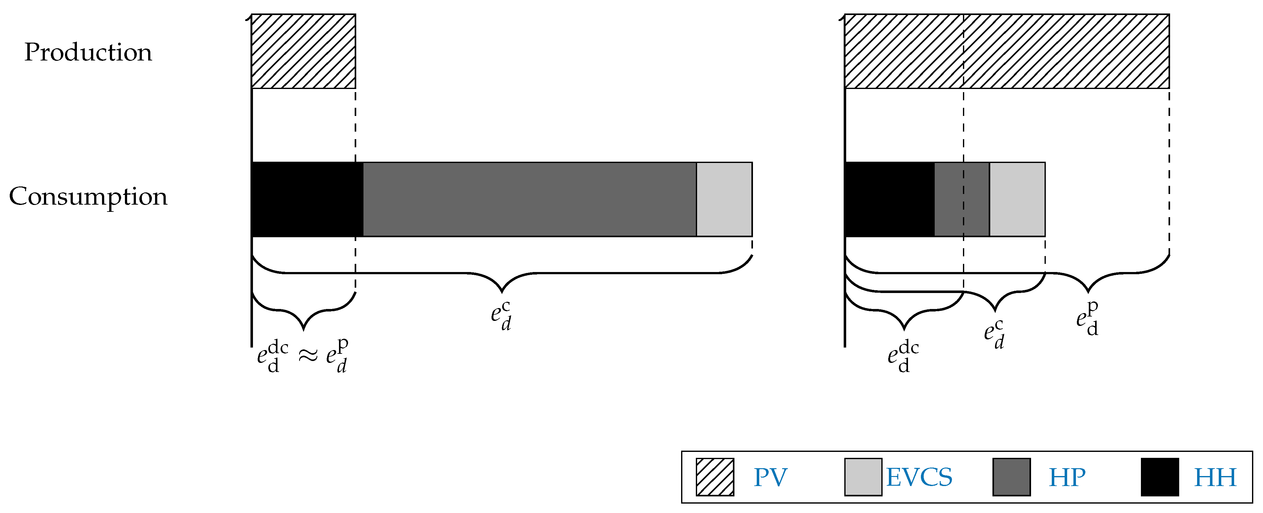
Once load profiles were defined, the next step was to determine the storage rates for the HHs. Due to the condition that stored energy is to be consumed within one day, no long-term storing was permitted. Therefore, the required storage size per household resulted from the sum of generation and consumption within one day. The storage rates for an exemplary HH on a winter day (left) and a summer day (right) are shown in Figure 2. Note that the figure represents the total daily energy consumption and production for HH, EVCS, HP and PV as well as the daily direct consumption $e_d^{\mathrm{dc}}$. During a summer day, more energy is produced by the PV system than can be consumed within a day. Storage operator’s intention is to store as much as can be consumed within a day. As a result, a parameter relevant for storage sizing was the sum of consumption minus the share that is directly consumed during the day. On a winter’s day, the reverse is true, and much more energy is consumed than can be produced in a day. As a result, storage sizing was calculated from the difference between production minus direct consumption. Since lithium-ion batteries are particularly suitable for stationary storage applications due to their high cycle stability as well as their low calendar ageing, the focus in this article was limited to them.

Equation (1) combines both approaches presented by finding the minimum between the potential charging energy and the potential discharging energy for each day.

$$e_d^{\mathrm{hh}}=\min \left(\left(\underset{\begin{array}{c}{e}_d^{\mathrm{c}}\end{array}}{\underbrace{{\displaystyle \sum _{t=1}^{24}}{p}_t^{\mathrm{c}}·\Delta t}}-\underset{\begin{array}{c}{e}_d^{\mathrm{dc}}\end{array}}{\underbrace{{\displaystyle \sum _{t=1}^{24}}{p}_t^{\mathrm{dc}}·\Delta t}}\right),\left(\underset{\begin{array}{c}{e}_d^{\mathrm{p}}\end{array}}{\underbrace{{\displaystyle \sum _{t=1}^{24}}{p}_t^{\mathrm{p}}·\Delta t}}-\underset{\begin{array}{c}{e}_d^{\mathrm{dc}}\end{array}}{\underbrace{{\displaystyle \sum _{t=1}^{24}}{p}_t^{\mathrm{dc}}·\Delta t}}\right)\right).$$

(1)

As part of the work, a monthly storage rate was developed for the HH. It enables the storage operator to have consistency for SU and at the same time a good adaptability for the households with regard to seasonal fluctuations. However, the benefit of a monthly adjustment of the storage rates can only be determined qualitatively in comparison to annual or daily storage rates. The storage operator daily storage rates imply a high degree of adaptability and a low degree of predictability of the surplus storage capacity. On the other hand, a constant annual storage rate does not show seasonal fluctuations and is therefore comparable to an HES. As a result, three possibilities for determining the storage space were distinguished:

• Yearly Storage Rate ($e_y^{⌀}$) The yearly storage rate is shown as a comparative value and represents the mean value of the daily storage rates. It is determined as the mean value of the daily storage rate of a year Y.

  $$e_y^{⌀}=\frac{1}{Y}·\sum _d{e}_d^{\mathrm{hh}}.$$

  (2)
• Monthly Storage Rate ($e_m^{⌀}$): The monthly storage rate represents the target of the contribution and is determined as the average storage rate per month m. Based on the daily storage rate of the households, the monthly storage rate can be determined from the relevant daily storage space by determining the mean value of all days in a month.

  $$e_m^{⌀}=\frac{1}{M}·\sum _{d\in (D\cap M)}{e}_d^{\mathrm{hh}}.$$

  (3)
• Daily Storage Rate ($e_d^{\mathrm{hh}}$): The daily storage rate represents the highest flexibility, but is difficult to realise for the storage operator. It has been already determined in (1) and subsequently used as a reference.

The monthly and yearly storage rates determined were used in the following as a basis for the evaluation of the added value for HHs and storage operators on the one hand, and as a data basis for the creation of the regression model on the other hand.

2.2. Determination of Added Value for Households and Storage Operators

In the previous section, the monthly and annual storage rate calculation was presented. Since the monthly allocation of storage associates effort and thus costs, the question arises of what added value it offers. With regard to households, the advantage of a monthly allocation was to be determined with the help of the indicators Self-Sufficiency Rate ($SSR$) and Self-Consumption Rate ($SCR$). In addition, the exceeding proportion can be used for secondary applications. These enable the storage operator to realise additional revenues. The potential for SU is shown by the monthly share as well as the daily share. The methods for determining the monthly and daily storage fractions are shown in Section 2.2.2.

2.2.1. Added Value for Households

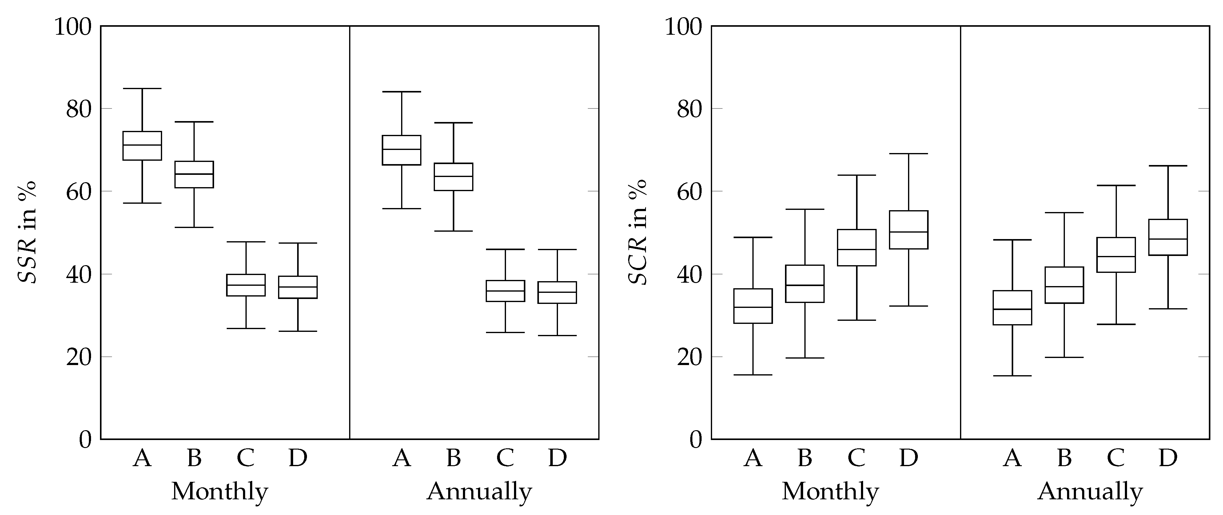
The benefits of monthly storage adaptations for HHs were evaluated using two indicators. The first indicator $SS{R}_{m/y}$ was based on the daily consumption, while the second indicator $SC{R}_{m/y}$ was based on the daily production. Both were calculated using the direct consumption and the stored energy $e_d^{\mathrm{s}}$ per day d. The stored energy can be determined on a monthly or an annual basis according to (4). If the daily storage rate exceeds the storage space, only the maximum possible capacity is stored. If the daily storage rate is less than the available storage space, it can be stored in full.

$$e_d^{\mathrm{s}}=\left\{\begin{array}{cccc}{e}_m^{⌀}& \mathrm{if}{e}_d^{\mathrm{hh}}\ge e_m^{⌀}\mathrm{or}& e_y^{⌀}& \mathrm{if}{e}_d^{\mathrm{hh}}\ge e_y^{⌀}\\ & & & \\ e_d^{\mathrm{hh}}& \mathrm{if}{e}_d^{\mathrm{hh}}<e_m^{⌀}\mathrm{or}& e_d^{\mathrm{hh}}& \mathrm{if}{e}_d^{\mathrm{hh}}<e_y^{⌀}\end{array}\right.$$

(4)

• Self-Sufficiency Rate ($SSR$): The degree of self-sufficiency describes the amount of self-consumption in relation to total electricity consumption.

  $$SS{R}_{m/y}=\sum _d\frac{e_d^{\mathrm{dc}}+e_d^{\mathrm{s}}}{e_d^{\mathrm{c}}}·100\%$$

  (5)
• Self-Consumption Rate ($SCR$): The degree of self-consumption describes the amount of self-consumption in relation to total electricity generation.

  $$SC{R}_{m/y}=\sum _d\frac{e_d^{\mathrm{dc}}+e_d^{\mathrm{s}}}{e_d^{\mathrm{p}}}·100\%$$

  (6)

2.2.2. Added Value for Storage Operators

Based on the average monthly storage rate of households storing energy. If there is more production, there is an export; if there is not enough energy in the storage, there must be an import. The analysis of [5] has shown that during the primary use to increase self-consumption, around 80% of the total capacity in a CES is secondarily not used. This means, there will be days when HHs do not call up their monthly storage rate. In addition to the monthly storage space, there will be months in which a portion of storage is not used for self-consumption. The variables $e_y^{⌀,\mathrm{su},\mathrm{I}}$, $e_y^{⌀,\mathrm{su},\mathrm{II}}$, $e_m^{⌀,\mathrm{su},\mathrm{I}}$ and $e_m^{⌀,\mathrm{su},\mathrm{II}}$ are calculated to investigate the exceed proportion of HH’s monthly storage rate according to (7)–(10). The two propositions can be separated as follows.

• Monthly Secondary Use Potential (SU,I): Denotes the share that is not used by HHs because of the monthly storage rate. Equation (7) determines the available storage per month for SU,I. To do this, it is important to know the month with the highest storage rate for HHs’ self-consumption. Afterwards, $e_m^{⌀,\mathrm{su},\mathrm{I}}$ can be calculated in each month m as the maximum monthly storage space minus the actual one. Note that the annual amount of $e_y^{⌀,\mathrm{su},\mathrm{I}}$ is zero, because there are no monthly variations.

  $$e_m^{⌀,\mathrm{su},\mathrm{I}}=max\left(e_m^{⌀}\right)-e_m^{⌀}.$$

  (7)
• Daily Secondary Use Potential (SU,II): Denotes the exceeded proportion of the daily storage rate. It can be determined by the storage rate in each day according to (8). Daily storage space is identified from the difference between the locked storage space $e_y^{⌀,\mathrm{su},\mathrm{II}}$ or $e_m^{⌀,\mathrm{su},\mathrm{II}}$ and actual storage rate $e_d^{⌀,\mathrm{su},\mathrm{II}}$. The excess storage space is zero if the household exhausts its available storage rate on that day. If the resident requires less storage (due to low PV feed-in or low consumption), the exceed proposition is available for the storage operator and can be used.

  $$e_d^{⌀,\mathrm{su},\mathrm{II}}=\left\{\begin{array}{cccc}0& \mathrm{if}{e}_d^{\mathrm{hh}}\ge e_m^{⌀}\mathrm{or}& 0& \mathrm{if}{e}_d^{\mathrm{hh}}\ge e_y^{⌀}\\ & & & \\ e_m^{⌀}-e_d^{\mathrm{hh}}& \mathrm{if}{e}_d^{\mathrm{hh}}<e_m^{⌀}\mathrm{or}& e_y^{⌀}-e_d^{\mathrm{hh}}& \mathrm{if}{e}_d^{\mathrm{hh}}<e_y^{⌀}.\end{array}\right.$$

  (8)

The monthly and annual potentials were thus finally calculated as shown in (9) for yearly or (10) for monthly investigations.

$$e_y^{⌀,\mathrm{su}}=\left(e_y^{⌀,\mathrm{su},\mathrm{I}}+e_y^{⌀,\mathrm{su},\mathrm{II}}\right)=0+\frac{1}{Y}·\sum _d{e}_d^{⌀,\mathrm{su},\mathrm{II}}$$

(9)

$$e_m^{⌀,\mathrm{su}}=\left(e_m^{⌀,\mathrm{su},\mathrm{I}}+e_m^{⌀,\mathrm{su},\mathrm{II}}\right)=e_m^{⌀,\mathrm{su},\mathrm{I}}+\frac{1}{M}·\sum _{d\in (D\cap M)}{e}_d^{⌀,\mathrm{su},\mathrm{II}}.$$

(10)

2.3. Determination of Storage Rate Using Multiple Linear Regression Coefficients

In the previous section, the monthly storage rate of the households was determined for the underlying data set and the method for determining the added value based on indicators was explained. However, the aim of this work was to develop a model that determines the necessary storage rates of households using simple parameters. For this purpose, multiple linear regression was used, which aims to explain the observed dependent variable (in our case $e_{m/y}^{⌀}$) by $n(n>1)$ independent variables $x_1,\dots ,x_n$ [40]. The model used for this purpose is linear, with the dependent variable being a function of independent variables. The regressor parameters ${\beta }_1,\dots ,{\beta }_n$ of the variables are determined by minimising the squared residuals. In the following, the annual electricity consumption of households ${\sum }_d{e}_d^{\mathrm{hh}}$ and the nominal power of the PV $p_{\mathrm{r}}^{\mathrm{PV}}$, of the EVCS $p_{\mathrm{r}}^{\mathrm{EVCS}}$ and of the HP $p_{\mathrm{r}}^{\mathrm{HP}}$ were examined as relevant independent variables for calculating the storage rates ${\widehat{e}}_{m/y}^{⌀}$. Note that both regressors for EVCS (${\beta }_{3,m/y}$) and HP (${\beta }_{4,m/y}$) were only taken into account when the profiles were activated in the corresponding case (case B–D).

The resulting regression equation can be derived according to (11) and (12).

$$e_{m/y}^{⌀}=\sum _d{e}_d^{\mathrm{hh}}·{\beta }_{1,m/y}+p_{\mathrm{r}}^{\mathrm{PV}}·{\beta }_{2,m/y}+p_{\mathrm{r}}^{\mathrm{EVCS}}·{\beta }_{3,m/y}+p_{\mathrm{r}}^{\mathrm{HP}}·{\beta }_{4,m/y}+\epsilon$$

(11)

$$e_{m/y}^{⌀}=\mathbf{X}·{\beta }_{m/y}+\epsilon .$$

(12)

The regression expression can be transformed into matrix form according to (12). Using the Gauss-Markov theorem, we obtain the best estimation for the regressors ${\beta }_{m/y}$. The estimated regression coefficients are shown in (13).

$${\widehat{\beta }}_{m/y}={({\mathbf{X}}^{\prime }·\mathbf{X})}^{-1}·{\mathbf{X}}^{\prime }·e_{m/y}^{⌀}.$$

(13)

The influence of the regression coefficients was examined with various statistical tests. We use the t-test for the significance of the regression coefficients. The null hypothesis $H_0$ states that $e_{m/y}^{⌀}$ is not explained by any model and if the p-value falls short of the predefined error (in our case 0.001%), the null hypothesis is rejected and the alternative hypothesis accepted. In this case, a second estimation was made and the p-values are checked by removing the regression coefficients that were rejected. In addition to the t-test, the multiple $R^2$ and the adjusted coefficient of determination $R^2$. For both tests, the results had high coefficients above 0.9 and can be provided upon request. Further information on the various test statistics can be found in [40].

3. Results and Discussion

Based on the method presented in Section 2, the question was answered of which advantages a monthly storage adjustment has. In addition, we dealt with the issue of how much storage is needed for different types of households for self-consumption optimisation. For this, the calculated monthly and annual storage rates are first presented in Section 3.1. Subsequently, Section 3.2 and Section 3.3 show the added values for households and storage operators and present and compare the multiple linear regression model.

3.1. Monthly and Annual Household’s Storage Rate‘s Calculation

Within the scope of this article, it is not possible to present all the data for the four cases studied. For this reason, a practical approach has been taken and, in addition to the general analyses, two example households were selected to demonstrate the results in a concrete application. The first household $hh1$ has an annual electricity consumption of $3.0\mathrm{MWh}/\mathrm{a}$ and an installed PV system capacity of $7.5\mathrm{kWp}$. For this household, the storage space required for the installation of a HP with $5.0\mathrm{kW}$ and the connection of a EVCS with $3.7\mathrm{kW}$ need to be investigated. In contrast, the second household $hh2$ has an annual electricity consumption of $4.0\mathrm{MWh}/\mathrm{a}$ with an installed PV system of $10\mathrm{kWp}$. The optional HP has a rated power of $7.0\mathrm{kW}$ and a EVCS connection with two charging points is to be investigated. A combination of HP and EVCS is conceivable in both households.

The monthly and annual storage rates for the two exemplary HHs are shown in Figure 3. Note that for both HHs all cases from Table 1 are shown (case A–D) and monthly as well as annual rates are illustrated. The annual storage rate is illustrated in both figures on the right hand side and it is highest for a HH with HP and EVCS (case D). If an additional electric vehicle is added, the optimal storage rate decreases in both exemplary HHs, as a larger part of the generated PV power is already used by the HP. For monthly rates in the base case with HH and PV, the common monthly structure for the storage rate is recognisable for both exemplary households. The storage rate increases in spring and autumn and decreases during summer and winter. The reduction in winter can be explained by the lower PV production, while the reduction in summer is caused by lower consumption. Once the residents have installed an EVCS, the storage rate will increase between March and October. The decrease in summer will also be compensated due to the rise in consumption. The relationship is more pronounced in case of $hh2$, where two charging points are installed. The most significant influence on the storage rate occurs when a HH is used, as shown by the comparison of the monthly storage rate in the baseline scenario (Case A) and the scenario with a HH (Case C). The storage rate increases in spring and autumn. Note that the storage rate more than triples in March and is 2.5 times higher in October. The high rise can be explained by the fact that the PV power generated during these periods is already higher than in winter and the storage rate of the HP is high due to the still cold season. In contrast, the storage rate in winter decreases due to the lower PV generation and the HP. In summer, the storage rate is low due to the lower consumption but higher than the case without HP due to the hot water demand. If the residents install both an HP and an EVCS, the two profiles will be combined. This leads to a slight decrease in the storage rate from November to March compared to the case without EVCS (case C). The reason for this is the higher base load during the day and therefore less PV power can be stored. In contrast, the storage rate from April to October will be increase by the EVCS. One reason is that during the summer months there is a surplus of PV production. The surplus energy is now stored and used to compensate the increase in consumption.

The monthly storage rates for the two HHs differ significantly from the annual storage rate. In the following, the benefits of adjusting the annual storage rate for HHs and storage operators were analysed. For this purpose, the indicators introduced in Section 2.2 were used.

3.2. Determination of Added Value for Households and Storage Operators

The four metrics used to assess the benefits for both were $SSR$ and $SCR$ as well as SU,I and SU,II, which were presented in Section 2. Households’ benefits were determined by the share of electricity that they can consume on their own ($SCR$) and the share of electricity that they do not import from the grid ($SSR$). In comparison, the storage operator sees the benefit in planning security for the surplus storage space in order to use it adequately on the market. To do so, the monthly and daily SU-potential of storage space was determined in the second part of Section 3.2.2. The indicators of the monthly storage rates could be reported separately for each month. However, to ensure the comparability of monthly and annual indicators, the monthly rates were related to a reference value. For this purpose, the average value was calculated out of the monthly rates. Please note that, in the context of this work, only the potential for a SU operation is indicated. Possible applications for a multi-use operation can be found in [7].

3.2.1. Determination of Added Value for Households

Figure 4 shows a comparison of the $SSR$ and $SCR$ of the households studied within one year. For this purpose, a distinction was made between a monthly and an annual storage rate. The left part of the respective figure shows the corresponding indicator for the monthly storage rate, while the right part shows the indicator with the annual storage rate. Three findings emerged from the comparison of the characteristic values (1) When consumption increases (case A–D), the $SSR$ decreases while the $SCR$ increases. (2) The increase in the $SCR$ is significantly more linear than the decrease in $SSR$. The decrease in $SSR$ is significantly influenced by the installation of a HP. (3) The results of the monthly storage rates are preferable across all configurations “−” for both $SSR$ and $SCR$.

By analysing both indicators in more detail, the SSR in the case without HP and EVCS has the highest value of $71.21\%$ on average for the monthly storage rate and $70.15\%$ for the annual storage rate. The deviation is comparatively small because the monthly fluctuations within the storage rate slices are also small. The HP has a dominant influence on the $SSR$, which causes the $SCR$ to drop to $37.29\%$ (monthly) and $35.88\%$ (annual). The marginal deviation of $1.41\%$ was not to be expected, but can be justified in the calculation of the indicator. It would be conceivable to significantly increase the installed PV power when using HPs in order to compensate for the drop. However, this will not be investigated further within the scope of this work.

In contrast, the denominator for $SCR$ remains constant and the positive influence is noticeable. The positive influence of additional load on the indicator (case B–D) can be explained by the fact that the self-consumed proportion of the annual generated PV power is determined. If consumption rises, the indicator also rises while generation remains constant. Moreover, the monthly storage rate is more targeted to the individual requests of the residents and thus additionally increases the indicator. The deviation between monthly and annual storage rates is approximately $1\%$, which is again a very small discrepancy.

The two exemplary households, for which the $SSR$ and $SCR$ in the different cases is illustrated in

Table 2. Average self-sufficiency rate and self-consumption rate of the exemplary households.

Case	hh 1				hh 2
	A	B	C	D	A	B	C	D
$SS{R}_m^{⌀}$	73.57%	68.08%	36.68%	36.68%	74.87%	63.67%	37.60%	37.18%
$SC{R}_m^{⌀}$	27.56%	32.04%	43.22%	46.77%	26.77%	37.33%	41.71%	46.45%
$SS{R}_y^{⌀}$	72.90%	67.76%	35.33%	35.44%	73.39%	63.16%	36.16%	35.44%
$SC{R}_y^{⌀}$	27.31%	31.89%	41.65%	45.19%	26.43%	37.03%	40.12%	44.86%

, will now serve as the basis for the analysis. Again for the two example households, the results of the two ratios for the monthly variation of the storage shares are higher than for an annual variation. The $SSR$ decreases over the cases while the $SCR$ increases over the cases. The significant drop by installing a HP from $73.57\%$ at the beginning to $36.68\%$ and $74.87\%$ to $37.60\%$ respectively is also detectable for the two sample households. Furthermore, by adding both HP and EVCS, the $SCR$ for $hh1$ and $hh2$ increase slightly, especially for the annual storage rate. Further results are presented in Table 2 and the added values of monthly storage shares for the storage operator are discussed in the next section.

3.2.2. Determination of Added Value for Storage Operators

Finally, the question of the added values for the storage operators should be answered. For this, the second use potential was introduced and converted into a monthly and a daily potential, as shown in (9) and (10). The comparison of monthly and daily potential as well as the necessary storage rate for self-consumption optimisation is shown in Figure 5.

Please note that the results in Figure 5 are related to the maximum monthly or yearly storage rate per HH and that only the average values are presented. Because of the relationship to the maximum monthly storage rate, SU,I and SU,II as well as the daily monthly storage rate must add up to $100\%$. In the base case without HP and EVCS, monthly storage rate $e_d^{\mathrm{hh}}$ is proportionally high and increases to $76.57\%$ for an annual storage rate. The monthly space for secondary use varies between 12.88% and 47.81% for $e_{m/y}^{⌀,\mathrm{su},\mathrm{I}}$ and between 9.32% and 27.42% for $e_{m/y}^{⌀,\mathrm{su},\mathrm{II}}$. The $e_{m/y}^{⌀,\mathrm{su},\mathrm{I}}$ is higher during the summer and winter months than in spring and autumn. This was to be expected as it is derived from the maximum storage rate (March) and is thus anti-cyclical to the storage rate itself. In contrast, the daily SU-potential $e_{m/y}^{⌀,\mathrm{su},\mathrm{II}}$ is high from November to February and comparatively low over the summer. For an installed EVCS, the relevant monthly storage rate remains comparable, but the monthly space for secondary use during the summer months is lower. Although the share for daily SU-potential compensates the adjustment, it also has a negative impact on the storage operator’s planning ability.

In the scenario of an installed HP (case C), HH’s storage rate increases significantly, as Figure 2 shows. Since Figure 5 shows the results in relation to the highest monthly storage rate, this share is assigned to the SU,I-potential. The SU,I potential varies between 4.56% (March) and 82.37% (December). Moreover, it is notable that the daily SU-potential $e_{m/y}^{⌀,\mathrm{su},\mathrm{II}}$ is higher in the case with HP if the monthly SU-potential is low. This is in contrast to the monthly potential for sales over the summer months (May to September), resulting in an average of $7.50\%$ $e_{m/y}^{⌀,\mathrm{su},\mathrm{II}}$ being available. The storage rate for monthly SU is much more pronounced over the same period at $58.45\%$. In the combined case with EVCS and HP (case D), the two above-described effects can be observed in combination. Thus, $e_{m/y}^{⌀,\mathrm{su},\mathrm{II}}$ in the summer months is strengthened by the EVCS and the monthly SU-potential is weakened. At the same time, the trend from October to March almost corresponds to the trend with HP only.

All in all, there is a clear dominant SU potential for monthly storage rates compared to annual storage rates in all four cases. While this can be partly justified by the higher storage rate of households (note that the basis of the calculation is the month with the highest monthly storage rate), the results also show the variation in the sales potential across months. The monthly SU potential ($e_m^{⌀,\mathrm{su},\mathrm{II}}$) is available to the storage operator for the entire month and known in advance.

Finally, the two example households were examined and the corresponding sales potentials are compared in

Table 3. Monthly and yearly second use potential for HH 1 and HH 2.

Case	HH 1				HH 2
	A	B	C	D	A	B	C	D
$e_m^{⌀,\mathrm{su},\mathrm{I}}$	24.70%	25.32%	53.47%	49.97%	22.77%	29.25%	52.29%	47.44%
$e_m^{⌀,\mathrm{su},\mathrm{II}}$	15.64%	18.95%	13.35%	14.78%	12.79%	18.52%	13.10%	15.41%
$e_y^{⌀,\mathrm{su},\mathrm{I}}$	−	−	−	−	−	−	−	−
$e_y^{⌀,\mathrm{su},\mathrm{II}}$	22.31%	26.11%	34.50%	34.91%	18.77%	27.33%	33.15%	34.38%

. In comparison to the results in Figure 5, Table 3 only shows the average values for the entire year for the monthly SU potential $e_{m/y}^{⌀,\mathrm{su},\mathrm{I}}$. Although $hh2$ has an annual electricity consumption of 4000 kWh per year and a higher installed PV power, in case A the SU-potential of the surplus monthly storage space is higher for $hh1$. Note that the values are only relative to the maximum monthly storage rate of the households. They are given in Figure 2 for the month with the maximum storage rate (e.g., March in case of HH, PV, HP). Additionally, by installing a HP, no surplus storage space can be sold from the larger $hh2$ compared to $hh1$ on a relative basis. Thereby, the monthly surplus storage increases to $53.47\%$ on average per year for the case with HP. In the cases with EVCS, the excess storage in $hh2$ is slightly higher than in $hh1$. Compared to the annual excess storage, the monthly excess storage dominates in all respects.

As a first conclusion, it can be stated that the benefit of monthly storage rates compared to annual storage rates is given for HHs and storage operators. The HHs achieve a higher SSR as well as a higher SCR through the monthly adjustment. Storage operators have greater reliability in planning their storage rates for SU and can also realise additional revenues through daily adjustments.

3.3. Multiple Linear Regressors for Household’s Storage Rate’s Calculation

Finally, a general model was created from the calculation of the storage rates using linear regression. This can be used in the future to determine the storage rate for a variety of CES. The annual electricity consumption of the HH ${\sum }_d{e}_d^{\mathrm{hh}}$, the installed peak power of the photovoltaic $p_{\mathrm{r}}^{\mathrm{PV}}$, and the nominal power of the EVCS $p_{\mathrm{r}}^{\mathrm{EVCS}}$ and HP $p_{\mathrm{r}}^{\mathrm{HP}}$ were examined as independent variables. Based on the regression coefficients, the storage rate of the HHs were estimated according to (13). The linear relationship is illustrated in (14). Please note that ${\widehat{e}}_{m/y}^{⌀}$ is the estimated storage rate.

$${\widehat{e}}_{m/y}^{⌀}=\sum _d{e}_d^{\mathrm{hh}}·{\widehat{\beta }}_{1,m/y}+p_{\mathrm{r}}^{\mathrm{PV}}·{\widehat{\beta }}_{2,m/y}+p_{\mathrm{r}}^{\mathrm{EVCS}}·{\widehat{\beta }}_{3,m/y}+p_{\mathrm{r}}^{\mathrm{HP}}·{\widehat{\beta }}_{4,m/y}.$$

(14)

3.3.1. Yearly Storage Calculation

In

Table 4. Multiple linear regression coefficients for the annual storage rates of the households.

Case	A = (HH, PV)		B = (HH, PV, EVCS)			C = (HH, PV, HP)			D = (HH, PV, EVCS, HP)
y	${\widehat{\beta }}_{1,y}^{\mathrm{A}}$	${\widehat{\beta }}_{2,y}^{\mathrm{A}}$	${\widehat{\beta }}_{1,y}^{\mathrm{B}}$	${\widehat{\beta }}_{2,y}^{\mathrm{B}}$	${\widehat{\beta }}_{3,y}^{\mathrm{B}}$	${\widehat{\beta }}_{1,y}^{\mathrm{C}}$	${\widehat{\beta }}_{2,y}^{\mathrm{C}}$	${\widehat{\beta }}_{4,y}^{\mathrm{C}}$	${\widehat{\beta }}_{1,y}^{\mathrm{D}}$	${\widehat{\beta }}_{2,y}^{\mathrm{D}}$	${\widehat{\beta }}_{3,y}^{\mathrm{D}}$	${\widehat{\beta }}_{4,y}^{\mathrm{D}}$
Year	0.870	0.123	0.790	0.158	0.221	0.534	0.283	0.282	0.801	0.107	0.331	0.182

, the regressors of the four cases from Table 1 from the annual storage calculation are compared. It can be seen that, in various cases, only some of the regressors have an influence on the storage size. This can be explained by the fact that another regressor takes over the necessary adjustment in the model. This is made clearer by looking at the effect of EVCS on the storage rate. Assuming exemplary $hh1$, the annual storage rate increases from $1.862\mathrm{kWh}$ in the base case (in detail: $3.0\mathrm{MWh}·0.870+7.5\mathrm{kWp}·0.123=1.862\mathrm{kWh}$) to $3.395\mathrm{kWh}$ in case of HH, PV and EVCS (in detail: $3.0\mathrm{MWh}·1.081+7.5\mathrm{kWp}·0.009+3.6\mathrm{kWp}·0.0236=3.395\mathrm{kWh}$). The influence of the nominal PV power on the storage size decreases significantly, while the influence of the annual electricity consumption ${\sum }_d{e}_d^{\mathrm{hh}}$ increases and the nominal power of the EVCS is considered. By installing a HP instead of the EVCS (case C), the influence of the annual electricity consumption decreases compared to the other regressors in the model.

3.3.2. Monthly Storage Calculation

The monthly storage rate model followed the same procedure as the annual storage rate model, while restricting the observed dependent variable to the respective month. In concrete terms, this means that a separate multiple linear regression model was created for each month. The values of the resulting regression coefficients are shown in

Table 5. Multiple linear regression coefficients for the monthly storage rates of the households.

Case	A = (HH, PV)		B = (HH, PV, EVCS)			C = (HH, PV, HP)			D = (HH, PV, EVCS, HP)
m	${\widehat{\beta }}_{1,m}^{\mathrm{A}}$	${\widehat{\beta }}_{2,m}^{\mathrm{A}}$	${\widehat{\beta }}_{1,m}^{\mathrm{B}}$	${\widehat{\beta }}_{2,m}^{\mathrm{B}}$	${\widehat{\beta }}_{3,m}^{\mathrm{B}}$	${\widehat{\beta }}_{1,m}^{\mathrm{C}}$	${\widehat{\beta }}_{2,m}^{\mathrm{C}}$	${\widehat{\beta }}_{4,m}^{\mathrm{C}}$	${\widehat{\beta }}_{1,m}^{\mathrm{D}}$	${\widehat{\beta }}_{2,m}^{\mathrm{D}}$	${\widehat{\beta }}_{3,m}^{\mathrm{D}}$	${\widehat{\beta }}_{4,m}^{\mathrm{D}}$
Jan.	0.435	0.284	0.326	0.332	0.061	0.084	0.451	−0.119	0.835	0.067	0.043	−0.136
Feb.	0.693	0.228	0.562	0.290	0.135	−0.155	0.637	0.176	0.953	0.097	0.069	0.116
Mar.	1.121	0.118	0.991	0.184	0.251	−	0.666	1.037	1.157	0.115	0.150	0.948
Apr.	1.158	0.047	1.100	0.073	0.266	1.012	0.115	0.530	1.201	0.031	0.235	0.500
May	1.162	−	1.126	0.016	0.205	1.059	0.047	0.329	1.134	0.013	0.195	0.318
Jun.	0.978	−	0.966	−	0.579	1.027	−0.025	0.232	0.988	−	0.568	0.210
Jul.	0.971	−	0.960	−	0.239	0.972	−	0.174	0.966	−	0.238	0.168
Aug.	0.994	0.045	0.957	0.051	0.338	1.008	0.036	0.106	1.042	0.010	0.335	0.097
Sep.	1.131	0.070	1.027	0.115	0.267	1.004	0.128	0.295	1.223	0.020	0.245	0.271
Oct.	0.934	0.179	0.825	0.230	0.176	0.387	0.440	0.601	1.147	0.069	0.130	0.556
Nov.	0.521	0.241	0.410	0.292	0.072	−	0.490	0.091	0.843	0.071	0.038	0.057
Dec.	0.313	0.275	0.227	0.313	0.061	−	0.422	−0.084	0.719	0.060	0.042	−0.102

. At first glance, it is clear that there is more variation in the coefficients and seasonal effects are considered in addition to the influence of the various inputs. Moreover, some regression coefficients have only a very small influence or can even be neglected (marked with “−”). This is the case, for example, in case A with PV and HH for the months May to July for ${\beta }_{2,m}^{\mathrm{A}}$. Whether there is a significant influence of the regressors on the monthly storage rate is checked using the t-test. If $H_0$ cannot be rejected for the corresponding regressor, a multiple linear regression model without the corresponding regressor takes place. If $H_0$ can subsequently be discarded, the corresponding regressor is assumed to be zero.

Different findings can be concluded from Table 5. In general, the strong influence of the annual electricity consumption ${\sum }_d{e}_d^{\mathrm{hh}}$ can be seen, except for the model with installed HP during winter. The influence of the installed PV power is low, especially in the summer months, and leads to the variable being assumed to be zero for HHs with EVCS during summer. In the winter months, however, the influence of the installed PV power is strong and is the dominating regression coefficient in the model with HP (case C) from October to March. By installing an EVCS, the storage rate is moderately increased in the months with more PV power available (March to October) and it is related to the monthly output of the photovoltaic system. Particularly during the winter months (December and January), the variable for the installed heat pump power is used to reduce the storage rate. This means that potential storage energy during both months is already consumed by the HP during day and only a smaller amount is stored.

3.3.3. Evaluation and Comparison of Regression Results

Finally, using the two example households, we then evaluated how well the results of the regression matched the previous results from the individual determination of the storage rate and what the annual storage rate was in comparison to the monthly storage rate. First, the storage rate must be determined using the regression coefficients from the previous section. For the example of $hh1$, the annual storage rate for HH with EVCS and HP is ${\widehat{e}}_y^{⌀}=6.24$ kWh (in detail: ${\widehat{e}}_y^{⌀}=4.0\mathrm{MWh}·0.801+10.5\mathrm{kWp}·0.170+7.4\mathrm{kW}·0.331+7\mathrm{kW}·0.182$). Note that the monthly storage rate can be calculated for both HH using the same procedure.

For the two exemplary households, Figure 6 compares the storage rates determined in the storage rate calculation with the estimated storage rates using the multiple linear regression model. The calculated storage rates from Section 2.1.3 are already shown in Figure 3 and were used as comparison values in this section. Four points stand out from the four cases studied and the comparison of the two sample households. First, it can be seen that $hh1$ can be estimated much more accurately than $hh2$. The discrepancy occurs for both the monthly and the annual storage rate. This suggests that smaller households are better estimated by the model than larger ones. This will be further investigated in future work. Secondly, the regression model can reproduce the monthly storage rate well. In the regression model, the months of April and October also show the highest storage rates. Storage rates decrease in summer and winter. Thirdly, the deviations in the case with EVCS tend to be higher than in the model with HP or in the base case (case A). In general, the regression without EVCS and HP shows the small deviations. In particular, $hh1$ is estimated very accurately, while $hh2$ tends to be underestimated from May to November (case A). Finally, in the fourth case with EVCS and HP, the January and April to June periods are inaccurately estimated. These deviations can be attributed to the disturbance variables of the multiple linear regression model. Overall, the results for determining the monthly and annual storage rate show that the model is easy to use. It only takes the input values from (14) to reliably determine the storage rate.

Finally, the question remains of whether multiple linear regression can be used to detect differences in determining monthly and annual storage. As expected, there are no anomalies and both concepts (monthly and annual) can be determined using the same data. All in all, the differences in size are clear when comparing the monthly and annual rates. While the annual rate is limited to a fixed value, the monthly storage rate varies between >200% and <50% of the annual storage rate.

4. Conclusions

In this article, focus was placed on the question of which monthly storage rate is required for various households. The goal was to find out general statements and to create added value for the simplified determination of the sizing for a community energy storage and thus to apply the profiles to many other districts. The first part of the article dealt with the advantages of adjusting the storage rate on a monthly basis. For this purpose, the degree of self-sufficiency and the self-consumption rate, as well as the monthly and daily potentials for secondary use, were shown and thus the added values for households and storage operators were demonstrated. The results show a consistently positive influence on the storage rate. Households can achieve a higher self-consumption rate through the monthly shares and thus consume their self-produced electricity in a more targeted manner. In addition, storage operators have increased planning security specifically due to the monthly storage rates. In the second part of the article, a multiple linear regression model was used, allowing us to determine the relevant monthly and annual storage rate of households from different independent variables. The result was a model which determines the storage rate of a households on the basis of the annual electricity consumption of households and the nominal power of the photovoltaic as well as of the electric vehicle charging station and of the heat pump. In the future, the results can be used for a first practical estimation of the necessary monthly and annual storage rate of residents in energetic communities. In this way, they serve to provide initial conclusions on the potentials of secondary marketing and can be seen as a first indication of the community energy storage size.

With regard to the limitations of the work, it should be pointed out that the profiles determined for the multiple linear regression correspond to different sources and were prepared for a potential district in Darmstadt, Germany. Additionally, the analysis was based on synthetic load profiles for generation and consumption. For a more targeted investigation of a potential secondary use, the requirements of a prequalification have to be taken into account and were included in the analysis.

The article leaves gaps for further and more detailed analyses in the field of the operation of storage systems. For example, the findings can be used to consider the necessary storage rates of households in the operation strategy of the storage system and to promote the secondary use of the excess storage capacity. It would also be possible to incorporate uncertainties in the storage rate into the analysis and develop a method using reinforcement learning. Lastly, the work can be used as a basis for designing a commercial strategy for monthly storage tariffs from the storage operator’s perspective, as in [41].

References

1. Verband der Elektrotechnik Elektronik Informationstechnik e.V. (VDE). VDE Study: “The Cellular Approach”; VDE/ETG Publication: Frankfurt, Germany, 2015. [Google Scholar]
2. Bayer, J.; Bögl, J.; Benz, T. Zellulares Energiesystem–Ein Beitrag zur Konkretisierung des Zellularen Ansatzes mit Handlungs-Empfehlungen; VDE-Technical Report; VDE-Energietechnische Gesellschaft (ETG): Frankfurt, Germany, 2019. [Google Scholar]
3. Wawer, T.; Griese, K.; Halstrup, D.; Ortmann, M. Community Electricity Storage: Current Challenges and Business Models in Germany. Z. Energ. 2008, 42, 225–234. [Google Scholar] [CrossRef]
4. Marczinkowski, H.M.; Østergaard, P.A. Residential versus communal combination of photovoltaic and battery in Smart Energy Systems. Energy 2018, 152, 466–475. [Google Scholar] [CrossRef]
5. Knoeffel, J.; Herrmann, B. Technisch-Ökonomische Bewertung von Quartierspeichern; Working Paper ESQUIRE Project; Esquire: Berlin, Germany, 2021; Available online: https://www.esquire-projekt.de/fileadmin/esquire/Datein/Knoefel_Herrmann_2021_Technisch_oekonomische_Bewertung_von_Quartierspeichern.pdf (accessed on 1 March 2023).
6. Meisenzahl, K.; Waffenschmidt, E. District Battery for Optimized Use of Photovoltaic Energy. In Proceedings of the 14th International Renewable Energy Storage Conference 2020 (IRES 2020), Online, 25–26 May 2020. [Google Scholar] [CrossRef]
7. Wiesenthal, J.; Schnabel, F. Multi-use of Community Energy Storage. In Proceedings of the 15th International Renewable Energy Storage Conference 2021 (IRES 2021), Online, 16–18 March 2021. [Google Scholar] [CrossRef]
8. Englberger, S.; Jossen, A.; Hesse, H. Unlocking the Potential of Battery Storage with the Dynamic Stacking of Multiple Applications. Cell Rep. Phys. Sci. 2020, 1, 100238. [Google Scholar] [CrossRef]
9. Elkazaz, M.; Sumner, M.; Naghiyev, E.; Hua, Z.; Thomas, D.W.P. Techno-economic sizing of a community battery to provide community energy billing and additional ancillary services. Sustain. Energy Grids Netw. 2021, 26, 100439. [Google Scholar] [CrossRef]
10. Dong, S.; Kremers, E.; Brucoli, M.; Rothman, R.; Brown, S. Improving the feasibility of household and community energy storage: A techno-enviro-economic study for the UK. Renew. Sustain. Energy Rev. 2020, 1310, 110009. [Google Scholar] [CrossRef]
11. Englberger, S.; Hesse, H.; Hanselmann, N.; Jossen, A. SimSES Multi-Use: A simulation tool for multiple storage system applications. In Proceedings of the 2019 16th International Conference on the European Energy Market (EEM), Ljubljana, Slovenia, 18–20 September 2019. [Google Scholar] [CrossRef]
12. Nourai, A.; Schafer, C. Changing the electricity game. IEEE Power Energy Mag. 2009, 7, 42–47. [Google Scholar] [CrossRef]
13. Sardi, J.; Mithulananthan, N.; Gallagher, M.; Hung, D.Q. Multiple community energy storage planning in distribution networks using a cost-benefit analysis. Appl. Energy 2017, 190, 453–463. [Google Scholar] [CrossRef]
14. Zhu, W.; Garrett, D.; Butkowski, J.; Wang, Y. Overview of distributive energy storage systems for residential communities. In Proceedings of the 2012 IEEE Energytech, Cleveland, OH, USA, 29–31 May 2012; pp. 1–6. [Google Scholar] [CrossRef]
15. Parra, D.; Walker, G.; Gillott, M. Modeling of PV generation, battery and hydrogen storage to investigate the benefits of energy storage for single dwelling. Sustain. Cities Soc. 2014, 10, 1–10. [Google Scholar] [CrossRef]
16. Van der Stelt, S.; AlSkaif, T.; Van Sark, W. Techno-economic analysis of household and community energy storage for residential prosumers with smart appliances. Appl. Energy 2018, 209, 266–267. [Google Scholar] [CrossRef]
17. Mignoni, N.; Scarabaggio, P.; Carli, R.; Dotoli, M. Control frameworks for transactive energy storage services in energy communities. Control. Eng. Pract. 2023, 130, 105364. [Google Scholar] [CrossRef]
18. Dai, R.; Esmaeilbeigi, R.; Charkhgard, H. The Utilization of Shared Energy Storage in Energy Systems: A Comprehensive Review. IEEE Trans. Smart Grid 2021, 12, 3163–3174. [Google Scholar] [CrossRef]
19. Venkatesan, K.; Govindarajan, U. Optimal power flow control of hybrid renewable energy system with energy storage: A WOANN strategy. J. Renew. Sustain. Energy 2019, 11, 015501. [Google Scholar] [CrossRef]
20. Zeh, A.; Müller, M.; Naumann, M.; Hesse, H.C.; Jossen, A.; Witzmann, R. Fundamentals of Using Battery Energy Storage Systems to Provide Primary Control Reserves in Germany. Batteries 2016, 2, 29. [Google Scholar] [CrossRef]
21. Schnabel, F.; Kreidel, K. Ökonomische Rahmenbedingungen für Quartierspeicher; Working Paper ESQUIRE Project; Esquire: Berlin, Germany, 2018; Available online: https://www.esquire-projekt.de/fileadmin/esquire/Datein/Schnabel_Arbeitspapier_%C3%B6konom._Rahmenbedingungen_Esquire.pdf (accessed on 1 March 2023).
22. HTW Berlin: Unabhängigkeitsrechner. Available online: https://solar.htw-berlin.de/rechner/unabhaengigkeitsrechner/ (accessed on 28 February 2023).
23. SENEC. Available online: https://www.speicher-rechnen.de/ (accessed on 28 February 2023).
24. HagerEnergy GmbH Osnabrück: E3/DC System Calculator. Available online: https://www.e3dc.com/konfigurator/ (accessed on 28 February 2023).
25. VARTA AG: Heimspeichersysteme Berechnungstool. Available online: https://www.varta-ag.com/de/konsument/produktkategorien/energiespeicher/berechnungstool (accessed on 28 February 2023).
26. Hesse, H.C.; Martins, R.; Musilek, P.; Naumann, M.; Truong, C.N.; Jossen, A. Economic Optimization of Component Sizing for Residential Battery Storage Systems. Energies 2017, 10, 835. [Google Scholar] [CrossRef]
27. Khezri, R.; Mahmoudi, A.; Aki, H. Optimal planning of solar photovoltaic and battery storage systems for grid-connected residential sector. Review, challenges and new perspectives. Renew. Sustain. Energy Rev. 2022, 153, 111763. [Google Scholar] [CrossRef]
28. Orth, N.; Weniger, J.; Meissner, L. Empfehlungen zur Auslegung von Solarstromspeichern: Welche Faustformeln helfen bei der Wahl der passenden Batteriekapazität in Einfamilienhäusern mit Photovoltaikanlagen? Sonnenenergie 2022, 2, 16–17. [Google Scholar]
29. Waffenschmidt, E.; Paulzen, T.; Stankiewicz, A. Common Battery Storage for an Area with Residential Houses. In Proceedings of the 13th International Renewable Energy Storage Conference 2019 (IRES 2019), Düsseldorf, Germany, 12–15 March 2019. [Google Scholar]
30. Barbour, E.; Parra, D.; Awwad, Z.; González, M.C. Community energy storage: A smart choice for the smart grid? Appl. Energy 2018, 212, 489–497. [Google Scholar] [CrossRef]
31. Guan, C.; Wang, Y.; Lin, X.; Nazarian, S.; Pedram, M. Reinforcement learning-based control of residential energy storage systems for electric bill minimization. In Proceedings of the 2015 12th Annual IEEE Consumer Communications and Networking Conference (CCNC), Las Vegas, NV, USA, 9–12 January 2015; pp. 637–642. [Google Scholar] [CrossRef]
32. Long, C.; Wu, J.; Zhang, C.; Cheng, M.; Al-Wakeel, A. Feasibility of Peer-to-Peer Energy Trading in Low Voltage Electrical Distribution Networks. Energy Procedia 2017, 105, 2227–2232. [Google Scholar] [CrossRef]
33. Cai, W.; Kordabad, A.; Gros, S. Energy management in residential microgrid using model predictive control-based reinforcement learning and Shapley value. Eng. Appl. Artif. Intell. 2023, 119, 105793. [Google Scholar] [CrossRef]
34. AlSkaif, T.; Luna, A.C.; Zapata, M.G.; Guerrero, J.M.; Bellalta, B. Reputation-based joint scheduling of households appliances and storage in a microgrid with a shared battery. Energy Build. 2017, 138, 228–239. [Google Scholar] [CrossRef]
35. Böhringer, M.; Kharrat, A.; Hanson, J.; Petermann, D.; Büchau, N.; Hein, C.; Baumann, S.; Preusche, C. Dimensioning of Community Energy Storages for Multi-Use Purposes using Households’ Storage Requirements. In Proceedings of the 57th International Universities Power Engineering Conference (UPEC), Istanbul, Turkey, 30 August–2 September 2022. [Google Scholar] [CrossRef]
36. Tjaden, T.; Bergner, J.; Weniger, J.; Quaschning, V. Repräsentative Elektrische Lastprofile für Wohngebäude in Deutschland auf 1-sekündiger Datenbasis. Available online: https://pvspeicher.htw-berlin.de/veroeffentlichungen/daten/lastprofile/ (accessed on 28 February 2023).
37. Huld, T.; Müller, R.; Gambardella, A. A new solar radiation database for estimating PV performance in Europe and Africa. Sol. Energy 2012, 86, 1803–1815. [Google Scholar] [CrossRef]
38. Meinecke, S.; Sarajlić, D.; Drauz, S.R.; Klettke, A.; Lauven, L.-P.; Rehtanz, C.; Moser, A.; Braun, M. SimBench—A Benchmark Dataset of Electric Power Systems to Compare Innovative Solutions Based on Power Flow Analysis. Energies 2020, 13, 3290. [Google Scholar] [CrossRef]
39. Böhringer, M.; Kharrat, A.; Steppan, R.; Schweinsberg, C.; Niersbach, B.; Hanson, J. Flexible Urban Medium Voltage Networks in the Darmstadt Energy Laboratory for Technology in Application (DELTA). Int. Etg Congr. 2023; accepted. [Google Scholar]
40. Toutenburg, T.; Schomaker, M.; Wißmann, M. Arbeitsbuch zur Deskriptiven und Induktiven Statistik, 2nd ed.; Springer: Berlin/Heidelberg, Germany, 2009; pp. 227–241. [Google Scholar] [CrossRef]
41. ENTEGA AG: Selbst Erzeugten Solarstrom Clever Zwischenspeichern. Der ENTEGA Quartierspeicher in Groß-Umstadt Macht es Möglich. Available online: https://www.entega.ag/fileadmin/downloads/quartierspeicher/ENTEGA-Quartierspeicher-komplett.pdf (accessed on 28 February 2023).
Figure 1. General methodology flow chart.
Electronics 12 02222 g001
Figure 2. Typical winter day (left) and summer day (right) for required household storage rates.
Electronics 12 02222 g002
Figure 3. Exemplary storage rates (monthly and yearly) for h h 1 (left) and h h 2 (right).
Electronics 12 02222 g003
Figure 4. Self-sufficiency rate S S R (left) and self-consumption rate S C R (right) of the examined cases.
Electronics 12 02222 g004
Figure 5. Second use potential for case A (top left), B (top right), C (bottom left) and D (bottom right).
Electronics 12 02222 g005
Figure 6. Comparison of the calculated (black) and estimated (grey) storage rates for the two exemplary households.
Electronics 12 02222 g006