High-Level Sensor Models for the Reinforcement Learning Driving Policy Training

Abstract

Performance limitations of automotive sensors and the resulting perception errors are one of the most critical limitations in the design of Advanced Driver Assistance Systems and Autonomous Driving Systems. Ability to efficiently recreate realistic error patterns in a traffic simulation setup not only helps to ensure that such systems operate correctly in presence of perception errors, but also fulfills a key role in the training of Machine-Learning-based algorithms often utilized in them. This paper proposes a set of efficient sensor models for detecting road users and static road features. Applicability of the models is presented on an example of Reinforcement-Learning-based driving policy training. Experimental results demonstrate a significant increase in the policy’s robustness to perception errors, alleviating issues caused by the differences between the virtual traffic environment used in the policy’s training and the realistic conditions.

1. Introduction

Advanced Driver Assistance Systems (ADAS) and Autonomous Driving Systems (ADS) possess the potential to significantly increase traffic safety by reducing the impact of human errors, which are by far the most common cause of accidents. Unfortunately, these systems do not come without their own risks—Highly Automated Vehicles (HAVs) may be susceptible to hardware and software malfunctions, as well as errors caused by the performance limitations of their perception systems. For these reasons HAVs require extensive validation and verification efforts to ensure that they meet their safety goals.

An intuitive way to assess the safety of ADAS/ADS and acquire data needed to develop and improve them is to use physical test drives. While this approach has been applied successfully for the development of ADAS features with a low level of autonomy, its application in HAVs poses a few severe challenges. End-to-end validation of ADS requires immense quantities of data to be gathered [1]. Furthermore, the development of certain ADAS/ADS algorithms, such as driving policies based on Reinforcement Learning (RL), requires triggering potentially dangerous behaviors and situations, which would be unacceptable to do in public traffic.

Traffic simulation tools are thus commonly utilized in the development and testing of ADAS/ADS [2]. The simulated road environment can be employed in both the open-loop testing, where actions of the vehicle equipped with the tested system, called the ego vehicle, do not impact the environment, and in closed-loop setups, where the traffic participants actively respond to the ego’s actions. The simulation is also a key component in RL-based driving policies training techniques, which typically utilize it to learn proper responses to various situations observed in the ego’s environment [3].

Both the testing and training applications require an accurate representation of the environment as perceived by automotive sensors, such as radars, LiDARs, or cameras. All of these sensors suffer however from various errors and performance degradation, that may be difficult to accurately recreate in a simulation environment. In this paper, I propose a set of high-level sensor models that can be used to realistically disturb the ground-truth descriptions of both the static and dynamic environments of the ego vehicle in a closed-loop simulation setup. Proposed models are applied to the RL-based driving policy training and their impact on the system’s performance is analyzed in a series of virtual driving experiments.

1.1. Related Work

Sensor models used for simulating the automotive perception systems can be most broadly assigned to two major classes: low-level sensor-specific models, that attempt to simulate error modalities of a particular sensor type, often through relatively precise simulation of underlying physical phenomena, and high-level generic models, that attempt to coarsely mimic perception errors through sensor-type-invariant statistical methods or heuristics.

Sensor-specific models of the automotive radar typically attempt to re-create error patterns related to physical properties of the radar wave, that lead to false-negative detections due to e.g., occlusions or weak reflections, and false positives caused by multi-path reflections of the wave. Depending on the computational resources and desired model’s accuracy, these phenomena may be either simulated using high-fidelity models in a relatively accurate manner, e.g., taking into account precise antenna characteristics [4], or approximated using statistical methods or low-fidelity models. High-fidelity methods include the use of the ray-tracing algorithms [5] that utilize geometric models of road users [6], often with pre-determined virtual scattering centers [7].

Due to the complexity of the radar modeling task and the nonlinear nature of the underlying models, Machine Learning techniques are often proposed to simulate radar’s error patterns. Muckenhuber et al. in [8] evaluate several machine-learning radar models trained on a labeled dataset. The authors of [9] utilize deep learning techniques to create a model that takes into account both static and dynamic environment features to produce a realistic model of the sensor’s output.

While the accurate simulation of underlying physical phenomena that impact radar sensors is a relatively complex task, high-fidelity simulation of the raw camera output can be performed by rendering the simulated scene and applying appropriate lens distortion models [10] and color space conversion [11]. It should be noted, however, that high-resolution rendering and execution of the camera’s object detection algorithms to produce an object list often require immense computational effort. Furthermore, acquiring high-quality results requires an accurate model of the environment, including 3D models of traffic participants, high-resolution textures, and realistic simulation of weather conditions.

Similarly, as in the case of radar sensor models, the use of machine learning techniques may help to achieve realistic output with a lower computational effort. Generative Adversarial Networks are often proposed for this task, due to their capability of producing realistically-looking images [12].

Due to the high computational cost of certain tasks that require sensor modeling, such as training of Reinforcement-Learning-based driving policies, low-fidelity models that operate on the object list instead of raw data are often proposed as an efficient alternative [13]. Object-level models may be also useful in situations where perception output incorporates a fusion of data from several types of sensors, and/or tracking algorithms. Examples of such setups include radar and vision fusion for detection of road barriers [14], road curbs tracking [15], and radar-camera sensor fusion for objects detection [16].

Analysis of the perception errors’ impact on driving policies is also an important area of research that utilizes sensor models. In [17], the authors proposed an error model for the LiDAR sensor and analyzed its impact on the control algorithms used for cooperative driving. [18] indicated that generic sensor models may play an important role in the training of Reinforcement-Learning-based driving policies, improving the robustness of the trained policy to the real-life performance limitations.

1.2. Motivation

The importance of sensor modeling in the validation and verification of the ADAS and AD systems is well understood, and models of various levels of fidelity are relatively commonly used in such applications. The emergence of the ADAS/AD algorithms based on Reinforcement Learning techniques poses however novel challenges related to the simulation and sensor modeling. Training of such algorithms often requires massive-scale simulations and the efficiency of the simulation and sensor models have a critical impact on the development of such systems.

While performance requirements in RL training setups suggest that the use of simple low-fidelity models, or even training the driving policies on ideal data is a desirable solution in this context, such a solution may contribute to the so-called sim-to-real gap. Differences between the simulated training environment and the real-world data streams may lead to the policy’s severe performance degradation when executed in the actual vehicle.

The impact of the sensor models on the RL training, performance of the driving policy, and overall safety of the AD system remain poorly understood. In this paper, I propose a set of low-fidelity sensor models intended to imitate errors in static and dynamic environment perception and apply them in the training of RL-based driving policy. Evaluation of the policy’s performance in various environments provides valuable insight into the sensor modeling’s impact on RL-based policies.

2. Sensor Models

Sensor modeling approaches vary with the required accuracy, computational resources available, type of sensor, and desired interfaces. While models proposed in this publication may find use in various applications, such as testing and performance evaluation of ADAS/AD algorithms, a main intended application is in the training of RL-based driving policies. The models are intended to operate on ground truth data provided by an arbitrary simulation package and modify them to reflect the typical performance of an automotive sensor stack and perception algorithms. The models are generic (not sensor-specific) and can be calibrated to reflect an arbitrary perception algorithm.

RL training usually requires gathering a massive amount of data in the simulation environment, resulting in a demand for highly effective, scalable simulation environments. For this reason, low-fidelity sensor models that do not have high computational requirements come across as an adequate solution. While low-fidelity models are typically less accurate compared to high-fidelity alternatives, RL-based driving policies tend to feature good generalization skills and do not require as a precise imitation of error profiles as perception performance evaluation applications.

2.1. Dynamic Environment Perception

Dynamic environment perception systems typically provide information about other traffic participants in the proximity of the ego vehicle, such as other vehicles and pedestrians. In this section, I propose models that can be used for various perception systems but are mainly intended to mimic the behavior of systems with time-correlated errors and frequent false positive and false negative detection errors. A good example of such a setup is a radar-based perception system that utilizes a tracking module to produce filtered object-level detections of road vehicles.

2.1.1. Interfaces

There is no common agreement on the simulation interfaces in the automotive industry, even though a few promising standards were already proposed, most notably the Open Simulation Interface [19]. Various simulation tools offer different output data formats, depending on the type of simulation and intended applications. RL-based driving policies typically utilize object lists that encode states of individual traffic participants separately for the dynamic environment description and various types of static environment representations, such as lane lists that gather information about road geometry or lane markers. This relatively high-level description of the vehicle’s environment is easy to process and does not create excessive bandwidth or memory requirements.

The low-fidelity sensor models presented in this paper utilize an interface that describes the ego’s dynamic environment as a list of dynamic objects that represent traffic participants such as vehicles. Dynamic environment at a time t in a scene composed of $n_d$ traffic participants is represented as a set of dynamic objects ${\mathbf{S}}_{\mathbf{d}}\left(t\right)={\left\{{\mathbf{S}}_{d_i}\left(t\right)\right\}}_{i=1..n_d}$, where each traffic participant is described with a state vector ${\mathbf{S}}_{\mathbf{d}i}\in {\mathbb{R}}^m,fori=1..n_d$ composed of m state variables:

$${\mathbf{S}}_{{\mathbf{d}}_{\mathbf{i}}}=\left[\begin{array}{c}\hfill {\mathbf{q}}_i\\ \hfill {\mathbf{x}}_i\\ \hfill {\psi }_i\\ \hfill v_i\\ \hfill a_i\end{array}\right],$$

(1)

where ${\mathbf{q}}_i\in {\mathbb{R}}^2$ denotes the size of the i-th traffic participant’s bounding box (length and width), ${\mathbf{x}}_i\in {\mathbb{R}}^2$ denotes its position in a Cartesian coordinates system, ${\psi }_i\in \mathbb{R}$ describes its rotation relative to the reference frame, $v_i\in \mathbb{R}$ denotes its absolute velocity, and $a_i\in \mathbb{R}$ denotes its absolute acceleration.

Observation of a dynamic scene representation ${\mathbf{S}}_d$ is generated by an arbitrary simulation package and processed by the sensor models to acquire an approximation of a perception stack’s dynamic environment estimate ${\widehat{\mathbf{S}}}_d={\left\{{\widehat{\mathbf{S}}}_{{\mathbf{d}}_{\mathbf{j}}}\right\}}_{j=1..n_o}$, composed of $n_o$ objects’ state estimates ${\widehat{\mathbf{S}}}_{d_j}={[{\widehat{\mathbf{q}}}_j,{\widehat{\mathbf{x}}}_j,{\widehat{v}}_j,{\widehat{a}}_j]}^T$.

Similarly as in the notation proposed by [20], the sensing process can be described as a mapping:

$$M\left(\mathbf{p}\right):{\left\{{\mathbf{S}}_{d_i}\right\}}_{i=1..n_d}\to {\left\{{\widehat{\mathbf{S}}}_{d_j}\right\}}_{j=1..n_o},$$

(2)

where $\mathbf{p}$ denotes sensor properties (calibration parameters). Note that during the sensing process certain objects may be omitted (false negative detections), while non-existing ones may be added (false positive detections), and thus, in general, ${\mathbf{S}}_{d_i}\nrightarrow {\widehat{\mathbf{S}}}_{d_i}$, and $n_d\ne n_o$.

As proposed in [20], sensing process M may be described as a series of $n_m$ mapping operations $M^{\left(k\right)}$ for $k=1..n_m$, yielding following sensor model:

$$M\left(\mathbf{p}\right)=M^{\left(n_m\right)}\left({\mathbf{p}}_{n_m}\right)\circ ...\circ M^{\left(2\right)}\left({\mathbf{p}}_2\right)\circ M^{\left(1\right)}\left({\mathbf{p}}_1\right)$$

(3)

where $M^{\left(n\right)}$ denotes the n-th mapping operation, and ${\mathbf{p}}_n$ is a vector of configuration parameters relevant to the n-th mapping operation. Note that configuration parameters may include the model’s outputs from previous observations if the mapping takes time correlations into account. n-th mapping operation can be defined as:

$$M^n\left({\mathbf{p}}_n\right):{\left\{{\mathbf{S}}_{\mathbf{d}i}\right\}}_{i=1..n_{k-1}}^{(k-1)}\to {\left\{{\mathbf{S}}_{\mathbf{d}j}\right\}}_{j=1..n_k}^{\left(k\right)},$$

(4)

where ${\left\{{\mathbf{S}}_{\mathbf{d}i}\right\}}_{i=1..n_{k-1}}^{\left(0\right)}$ is equal to the ground-truth description of the dynamic environment ${\mathbf{S}}_d$, and ${\left\{{\mathbf{S}}_{\mathbf{d}j}\right\}}_{j=1..n_k}^{\left(k\right)}$ corresponds to the approximation of the sensing stack’s dynamic environment’s estimate ${\widehat{\mathbf{S}}}_{\mathbf{d}}$, while $n_k$ denotes the number of objects after k-th mapping operation.

2.1.2. Model of Dynamic Environment Perception Stack

The low-fidelity model of a dynamic environment perception stack is intended to imitate the main error types observed in object-detection systems used in automotive. A common example of such system is a set of short-range millimeter-wave Phase-Modulated Continuous Wave (PMCW) Radars placed in the vehicle’s corners and a long-range PMCW radar in the front of the vehicle. Data from the sensors, for instance in a form of object lists, is typically fused using tracking algorithms based on derivatives of a Kalman Filter.

Errors commonly observed in such systems can be roughly assigned to the categories listed below.

• False positive detections.Various physical phenomena, such as multipath reflections of a radar wave, may result in an introduction of non-existing objects to the object list ${\widehat{\mathbf{S}}}_d$, leading to the situation in which ADAS/AD algorithms assume the presence of potentially dangerous objects in unoccupied areas.
• False negative detections. Limited performance of the sensors, as well as performance degradations caused by difficult environmental conditions such as bad weather, may lead to missed object detections, i.e., situations in which a dynamic object present in ego’s vicinity is not represented in the object list ${\widehat{\mathbf{S}}}_d$.
• State estimation errors. Partial occlusions and performance degradations may lead to potentially dangerous differences between ground truth state description ${\mathbf{S}}_{d_i}$ of a particular object, and its estimate ${\widehat{\mathbf{S}}}_{d_i}$ composed by the sensor stack. It should be noted, that due to the filtering properties of the tracking algorithm, state estimation errors may be time-correlated.

Differences between the ground truth ${\mathbf{S}}_{\mathbf{d}}$ and the estimate ${\widehat{\mathbf{S}}}_{\mathbf{d}}$ may also be caused by the range and angle limitations of the sensors, as well as occlusions.

Before modeling stochastic errors related to the sensors’ performance, deterministic sensors’ limitations are modeled according to the specification of the sensor stack. Objects that are outside of the sensors’ detection area are removed from the ground-truth objects list. Similarly, objects that are occluded or partially occluded by other traffic participants or obstacles can be removed. These operations are denoted as $M^v\left({\mathbf{p}}_v\right):{\left\{{\mathbf{S}}_{\mathbf{d}i}\right\}}_{i=1..n_d}\to {\left\{{\mathbf{S}}_{\mathbf{d}j}\right\}}_{j=1..n_v}^{\left(v\right)}$, where calibration parameters ${\mathbf{p}}_v$ describe the sensing stack’s detection area and the occlusion level above which the object is removed, while $n_v$ denotes the number of the unoccluded objects in the detection area.

Two types of false negative object detections are simulated in the proposed generic sensor models. The first type is the detection delay. Due to the latencies in the vehicle’s internal communication network, as well as properties of the tracking algorithms, that often need to confirm the existence of the object in a few consecutive scans before adding it to the object list, a random delay between the object entering the sensors’ detection area and actually detecting it can be observed in the most of the sensor stacks. This property of the sensing system is modeled by assigning a random detection delay of $T_{d_i}$ for $i=1..n_v$ seconds to each object newly introduced to the ${\left\{{\mathbf{S}}_{\mathbf{d}i}\right\}}_{i=1..n_d}$ set, which value is sampled from a normal distribution:

$$T_{d_i}=max\left(p_{d_{\mu \_delay}},|\sim \mathcal{N}(0,p_{d_{\sigma \_delay}}^2)|\right),$$

(5)

where $p_{\mu \_delay}$ and $p_{\sigma \_delay}$ are calibration parameters.

Additionally, to model random losses of already detected objects, each object at each sensing update can be marked as a false-negative detection with a certain probability $p_{d\_fn\_prob}$, and assigned a $T_f=max\left(p_{fn\_\mu },|\sim \mathcal{N}(0,p_{fn\_\sigma }^2)|\right)$ value that denotes duration for which it will remain marked as a false-negative. Parameters $p_{\mu \_\mathrm{delay}}$, $p_{\sigma \_\mathrm{delay}}$, $p_{\mathrm{fn}\_\mathrm{prob}}$, $p_{\mathrm{fn}\_\mu }$, $p_{\mathrm{fn}\_\sigma }$, as well as detection delays $T_{d_i}$, false-negative flags, detection durations $T_f$, current timestamp and timestamps at which objects were first observed or marked as false-negatives are included in the parameters vector ${\mathbf{p}}_{\mathbf{d}}$, allowing to remove objects that are newly detected and marked as a false-negative in a following mapping:

$$M^d\left({\mathbf{p}}_d\right):{\left\{{\mathbf{S}}_{\mathbf{d}i}\right\}}_{i=1..n_v}^{\left(v\right)}\to {\left\{{\mathbf{S}}_{\mathbf{d}j}\right\}}_{j=1..n_{d}d}^{\left(d\right)}.$$

(6)

False positive detection errors, especially in radar sensors, often exhibit behavior similar to actual road users, posing a serious challenge to ADAS/AD systems. In the proposed approach, a false positive object can be introduced to the sensed objects set with a probability $p_{\mathrm{fp}\_\mathrm{prob}}$. Since false positive detection errors often persist for multiple sensing updates, duration $T_{fp}=max\left(p_{\mathrm{fp}\_\mu },|\sim \mathcal{N}(0,p_{\mathrm{fp}\_\sigma }^2)|\right)$ is assigned to the newly introduced false positive object, during which the object will persist in the dynamic scene approximation set. A newly created object is initialized with a random state ${\mathbf{S}}_{fn}$, which values are sampled from normal distributions:

$${\mathbf{S}}_{\mathbf{fp}}=\left[\begin{array}{c}\hfill \mathbf{q}\sim {\mathcal{N}}_2({\mu }_q,{\mathsf{\Sigma }}_q)\\ \hfill \mathbf{x}\sim {\mathcal{N}}_2({\mu }_x,{\mathsf{\Sigma }}_x)\\ \hfill \psi \sim \mathcal{N}({\mu }_{\psi },{\sigma }_{\psi })\\ \hfill v\sim \mathcal{N}({\mu }_v,{\sigma }_v)\\ \hfill a\sim \mathcal{N}({\mu }_a,{\sigma }_a)\end{array}\right],$$

(7)

where ${\mu }_q$, ${\mathsf{\Sigma }}_q$, ${\mu }_x$, ${\mathsf{\Sigma }}_x$, ${\mu }_{\psi }$, ${\sigma }_{\psi }$, ${\mu }_v$, ${\sigma }_v$, ${\mu }_a$, and ${\sigma }_a$, are the calibration parameters included in the parameters vector ${\mathbf{p}}_p$. All of the false positive objects are assumed to move in the direction of their orientation $\psi$ with a constant acceleration, and thus their state (included in the parameters vector ${\mathbf{p}}_p$) is updated according to these assumptions at each sensing update.

Operations of false positive objects creation, update, and removal after corresponding $T_{fp}$ are denoted as the following mapping:

$$M^p\left({\mathbf{p}}_p\right):{\left\{{\mathbf{S}}_{\mathbf{d}i}\right\}}_{i=1..n_{dd}}^{\left(d\right)}\to {\left\{{\mathbf{S}}_{\mathbf{d}j}\right\}}_{j=1..n_p}^{\left(p\right)}.$$

(8)

Lastly, state estimation errors are introduced. State errors in the automotive perception systems tend to be time-correlated due to the filtering properties of tracking and fusion algorithms used in them, as well as due to the persistency of environmental triggers (it is rare for an environmental trigger to impact only a single perception update). In order to reflect the randomness of the errors, as well as their time-correlated nature, a multivariate stochastic process based on the Ornstein–Uhlenbeck process is utilized for state values modeling. The value of an $n_c$-dimensional state estimate vector chunk ${\widehat{\mathbf{s}}}_c$ at i-th perception update is calculated according to the process:

$$P_{O{U}_c}\left({\widehat{\mathbf{s}}}_c^{\left(i\right)}\right|{\mathbf{s}}^{\left(i\right)},{\widehat{\mathbf{s}}}^{(i-1)},{\mathbf{p}}_{s_c})=\left\{\begin{array}{cc}{\mathbf{p}}_{\mathrm{ou}\_{\lambda }_c}\ast ({\mathbf{s}}^{\left(i\right)}-{\widehat{\mathbf{s}}}^{(i-1)})\ast dt+{\mathbf{W}}^{\left(i\right)}\ast dt,\hfill & \mathrm{for}i>1\hfill \\ {\mathcal{N}}_{n_c}({\mathbf{s}}^{\left(i\right)},{\mathbf{p}}_{\mathrm{ou}\_\mathsf{\Sigma }\_{\mathrm{init}}_c}),\hfill & \mathrm{for}i=0,\hfill \end{array}\right.$$

(9)

where ${\mathbf{s}}^{\left(i\right)}\in {\mathbb{R}}^{n_c}$ is the ground-truth value at i-th perception update, ${\widehat{\mathbf{s}}}^{(i-1)}\in {\mathbb{R}}^{n_c}$ is the previous value of state estimate, $dt$ is the time between perception updates, and ${\mathbf{W}}_i\in {\mathbb{R}}^{n_c}$ is drawn from a multivariate normal distribution ${\mathbf{W}}_i\sim {\mathcal{N}}_{n_c}(\mathbf{0},{\mathbf{p}}_{\mathrm{ou}\_\mathsf{\Sigma }\_u_c})$. ${\mathbf{p}}_{\mathrm{ou}\_{\lambda }_c}$, ${\mathbf{p}}_{\mathrm{ou}\_\mathsf{\Sigma }\_{\mathrm{init}}_c}$ and ${\mathbf{p}}_{\mathrm{ou}\_\mathsf{\Sigma }\_u_c}$ are the calibration parameters included in the vector ${\mathbf{p}}_{s_c}$.

The state of the dynamic environment is updated according to the mapping:

$$M^{\mathrm{state}\_\mathrm{est}}({\mathbf{p}}_{\mathrm{state}\_\mathrm{est}},{\mathbf{S}}_{\mathrm{state}\_\mathrm{est}}^{(t-1)}):{\left\{{\mathbf{S}}_{\mathbf{d}i}\right\}}_{i=1..n_{dd}}^{\left(d\right)}\to {\left\{{\mathbf{S}}_{{\mathrm{state}\_\mathrm{est}}_j}^{\left(t\right)}\right\}}_{j=1..n_p}^{\left(p\right)},$$

(10)

where ${\mathbf{S}}_{{\mathrm{state}\_\mathrm{est}}_j}^{\left(t\right)}$ is calculated using a process:

$${\mathbf{S}}_{{\mathrm{state}\_\mathrm{est}}_j}^{\left(t\right)}=P_{OU}({\widehat{\mathbf{S}}}^{\left(\mathbf{t}\right)}|{\mathbf{S}}^{\left(t\right)},{\widehat{\mathbf{S}}}^{(t-1)},{\mathbf{p}}_{\mathrm{state}}),$$

(11)

parameterized with a vector ${\mathbf{p}}_{\mathrm{state}}$ consisting of ${\mathbf{p}}_{\mathrm{ou}\_\lambda }$, ${\mathbf{p}}_{\mathrm{ou}\_\mathsf{\Sigma }\_\mathrm{init}}$ and ${\mathbf{p}}_{\mathrm{ou}\_\mathsf{\Sigma }\_u}$ calibration matrices.

The final model can be described as the mapping:

$$M_r\left(\mathbf{p}\right)=M^{\left(v\right)}\left({\mathbf{p}}_v\right)\circ M^{\left(d\right)}\left({\mathbf{p}}_d\right)\circ M^{\left(p\right)}\left({\mathbf{p}}_p\right)\circ M^{\mathrm{state}\_\mathrm{est}}\left({\mathbf{p}}_{\mathrm{state}\_\mathrm{est}}\right).$$

(12)

The proposed model, depending on the calibration parameters, may imitate an arbitrary dynamic environment perception system, including false positive and false negative errors, as well as time-correlated state perception errors. Values of calibration parameters used in a further evaluation are provided in Appendix A.

2.2. Static Environment Perception

Features of a static environment of the ego vehicles relevant to ADAS/AD algorithms can be categorized into two main types: road features such as the geometry of the road, lane markers or barriers, and static obstacles such as parked cars, or debris. Since static obstacle detection is often based on similar sensor stack and perception algorithms as the dynamic environment perception, they can be represented using the ${\mathbf{S}}_d$ state vector with reasonable accuracy. Depending on the object type, $\widehat{v}$ and $\widehat{a}$ may be set to 0, though in certain situations allowing for non-zero velocity and acceleration may be desirable to reflect potential errors e.g., in state estimation of recently stopped or potentially moving vehicles.

The road features most relevant to RL-based driving policies are represented as a set ${\mathbf{S}}_{\mathbf{r}}\left(t\right)={\left\{{\mathbf{S}}_{r_i}\left(t\right)\right\}}_{i=1..n_s}$ composed of $n_s$l-dimensional vectors ${\mathbf{S}}_{\mathbf{r}i}\in {\mathbb{R}}^{l}fori=1..n_s$ representing lane markers in the vicinity of the ego vehicle. Each vector describes a single lane marker in a following form:

$${\mathbf{S}}_{{\mathbf{r}}_{\mathbf{i}}}=\left[\begin{array}{c}\mathbf{c}\\ h\end{array}\right],$$

(13)

where $\mathbf{c}\in {\mathbb{R}}^4$ denotes coefficients $\mathbf{c}=\left[c_0,c_1,c_2,c_3\right]$ of a cubic polynomial $d\left(s\right)=c_3\ast s^3+c_2\ast s^2+c_1\ast s+c_0$ that encodes the lateral offset d of a lane marking (road edge or line) from the vehicle’s longitudinal axis as a function of a longitudinal distance from the vehicle’s rear axis, and h denotes the longitudinal distance up to which the lane marking is observed. Similarly, as in the case of the dynamic environment, the ground truth of the static scene representation ${\mathbf{S}}_{r_i}\left(t\right)$ is generated by a simulation package and processed by the static environment sensor models to acquire an approximation of a perception stack’s static environment estimate ${\widehat{\mathbf{S}}}_r({\mathbf{S}}_r,\mathbf{p},t)$ composed of an arbitrary number of lane markers state estimates ${\widehat{\mathbf{S}}}_{r_i}\left(t\right)={\left[\widehat{\mathbf{c}}\left(t\right),\widehat{h}\left(t\right)\right]}^T$.

The sensing process for the static environment can be thus modeled as a series of mapping operations:

$$M_r\left(\mathbf{d}\right)=M_r^{\left(n_m\right)}\left({\mathbf{d}}_{n_m}\right)\circ ...\circ M_r^{\left(2\right)}\left({\mathbf{d}}_2\right)\circ M_r^{\left(1\right)}\left({\mathbf{d}}_1\right),$$

(14)

defined analogically to the mappings proposed for the dynamic environment sensing model.

Model of Static Environment Perception Stack

Static environment errors modeled in the proposed approach include marker length limitations (e.g., due to occlusions or detection performance limitations), false negative detections, and geometry estimation errors.

The detection range limitation model is intended to imitate the lane detection quality decrease on long distances due to the perspective, occlusions, and environmental factors such as fog or rain. It should be noted that the range limitation impacts the quality of lane markers geometry estimation - the model assumes that the lane marker geometry can be estimated solely based on the part of the lane assumed to be visible.

The model uniformly samples the ground truth lane markers geometries ${\mathbf{S}}_r$, mapping each lane marker definition ${\mathbf{S}}_{r_i}$ to a set ${\left\{{\mathbf{s}}_i\right\}}_{j=1..n_{samples}}$ of samples ${\mathbf{s}}_{i_j}={[x_s,y_s]}^T$, where $x_s$ and $y_s$ are the longitudinal and lateral position of the lane marker sample in the Vehicle Coordinates System (VCS). The occlusion model is defined as a mapping:

$$M^{\left(\mathrm{occ}\right)}\left({\mathbf{p}}_{\mathrm{occ}}\right):{\left\{{\mathbf{s}}_i\right\}}_{j=1..n_{\mathrm{samples}}}\to {\left\{{\mathbf{s}}_i^{\mathrm{occ}}\right\}}_{j=1..n_{\mathrm{occ}}}$$

(15)

evaluates whether each lane sample is occluded by any of the dynamic objects from the ${\mathbf{S}}_d$ set and discards them from the final samples set ${\left\{{\mathbf{s}}_i^{\mathrm{occ}}\right\}}_{j=1..n_{\mathrm{occ}}}$. If at least $n_{\mathrm{cons}}$ consecutive samples in a lane marker are occluded, all of the samples placed farther from the vehicle are discarded as well.

The distance of the farthest sample from each lane marker from the set is treated as a base marker length $h_{gt}$. The value of the marker length is calculated similarly to dynamic objects state estimates, using a stochastic model based on the Ornstein–Uhlenbeck process:

$$P_h({\widehat{h}}^{\left(t\right)}|h_{gt}^{\left(t\right)},h_{gt}^{(t-1)},{\widehat{h}}^{(t-1)},{\mathbf{p}}_h)=\left\{\begin{array}{c}\left(p_{\mathrm{lm}\_\mathrm{ou}\_\lambda \_h}\left(\left(h_{gt}^{\left(t\right)}-p_{\mathrm{lm}\_\lim }\right)-{\widehat{h}}^{(t-1)}\right)+W^{\left(t\right)}\right)\ast dt\hfill \\ \hfill \mathrm{if}t>0\mathrm{and}\left(h_{gt}^{\left(t\right)}-h_{gt}^{(t-1)}\right)\ge p_{\mathrm{lm}\_\mathrm{jump}}\hfill \\ \mathcal{N}\left(h_{gt}^{\left(t\right)}-p_{\mathrm{lm}\_\lim },p_{\sigma \_h}\right)\hfill \\ \hfill \mathrm{otherwise},\hfill \end{array}\right.$$

(16)

where $p_{\mathrm{lm}\_\mathrm{ou}\_\lambda \_h}$, $p_{\mathrm{lm}\_\lim }$, $p_{\mathrm{lm}\_\mathrm{jump}}$, and $p_{\sigma \_h}$ are the calibration parameters included in parameters vector ${\mathbf{p}}_h$. Note that if the ground truth lane length is severely decreased between the time updates, i.e., $\left(h_{gt}^{\left(t\right)}-h_{gt}^{(t-1)}\right)\ge p_{\mathrm{lm}\_\mathrm{jump}}$, the Ornstein-Uhlenbeck process is reset, and the length value is drawn from a normal distribution to more accurately model sudden lane occlusions.

The geometry of the lane markers is calculated using a mapping $M^{\left(geom\right)}({\mathbf{p}}_c,{\mathbf{p}}_h)$, that calculates the geometry of lane markers as:

$${\mathbf{S}}_j^{\left(t\right)}=\left[\begin{array}{c}\hfill P_{OU}({\widehat{\mathbf{c}}}^{\left(t\right)}|{\mathbf{c}}^{\left(t\right)},{\widehat{\mathbf{c}}}^{(t-1)},{\mathbf{p}}_{\mathbf{c}})\\ \hfill P_{OU}({\widehat{h}}^{\left(t\right)}|h_{gt}^{\left(t\right)},h_{gt}^{(t-1)},{\widehat{h}}^{(t-1)},{\mathbf{p}}_h)\end{array}\right]\mathrm{for}j=1..n_{\mathrm{occ}},$$

(17)

where ${\mathbf{p}}_c$ is a vector of calibration parameters, consisting of calibration matrices ${\mathbf{p}}_{\mathrm{lm}\_\mathrm{ou}\_\lambda }$, ${\mathbf{p}}_{\mathrm{lm}\_\mathrm{ou}\_\mathsf{\Sigma }\_\mathrm{init}}$ and ${\mathbf{p}}_{\mathrm{lm}\_\mathrm{ou}\_\mathsf{\Sigma }\_u}$.

Finally, the false negative lane markers detection model is applied. The model is based on intuition, that lane markers with a higher lateral offset from the ego vehicle, as well as shorter (occluded) ones, have a higher probability of being not detected by the perception system. Lane offset $o\in \mathbb{N}$ denotes the number of lane markers between the ego vehicle and the given marker, where $o=0$ corresponds to a lane marker on either the left or right side of the ego’s current lane.

The mapping $M^{\mathrm{fp}}\left({\mathbf{p}}_{\mathrm{fp}}\right):{\left\{{\mathbf{S}}_i^{\mathrm{geom}}\right\}}_{i=1..n_{geom}}\to {\left\{{\mathbf{S}}_j^{\mathrm{fp}}\right\}}_{j=1..n_{\mathrm{fp}}}$ is randomly discarding lane markers according to the probability $P_{\mathrm{discard}}$:

$$P_{{\mathrm{discard}}_i}\left({\mathbf{p}}_{\mathrm{fn}}\right)=\left\{\begin{array}{cc}{p}_{\lim \_\mathrm{disc}\_\mathrm{c}\_0}+p_{\lim \_\mathrm{disc}\_\mathrm{l}\_0}\ast \frac{h_{\max }-h_i}{h_{\max }}\hfill & \mathrm{if}o=0\hfill \\ p_{\lim \_\mathrm{disc}\_\mathrm{c}\_1}+p_{\lim \_\mathrm{disc}\_\mathrm{l}\_1}\ast \frac{h_{\max }-h_i}{h_{\max }}\hfill & \mathrm{if}o=1\hfill \\ p_{\lim \_\mathrm{disc}\_\mathrm{c}\_2}+p_{\lim \_\mathrm{disc}\_\mathrm{l}\_2}\ast \frac{h_{\max }-h_i}{h_{\max }}\hfill & \mathrm{otherwise},\hfill \end{array}\right.\mathrm{for}i=1..n_{\mathrm{geom}},$$

(18)

where $p_{\lim \_\mathrm{disc}\_\mathrm{c}\_0}$, $p_{\lim \_\mathrm{disc}\_\mathrm{l}\_0}$, $p_{\lim \_\mathrm{disc}\_\mathrm{c}\_1}$, $p_{\lim \_\mathrm{disc}\_\mathrm{l}\_1}$, $p_{\lim \_\mathrm{disc}\_\mathrm{c}\_2}$, and $p_{\lim \_\mathrm{disc}\_\mathrm{l}\_2}$ are the calibration parameters included in the parameters vector ${\mathbf{p}}_{\mathrm{fn}}$, and $h_{\max }$ denotes the maximum length of the lane marker that can be detected by the modeled perception system.

Discarded lane markers remain false negatives, with a probability $P_{\mathrm{lm}\_\mathrm{recovery}}$ of returning to their true positive state on each perception update:

$$P_{\mathrm{lm}\_\mathrm{recovery}}=p_{\mathrm{rec}\_\mathrm{hyst}}\ast (1-P_{\mathrm{discard}})+min(p_{\mathrm{rec}\_\mathrm{pps}}\ast t_{\mathrm{disc}},p_{\mathrm{rec}\_\mathrm{sat}}),$$

(19)

where $t_{\mathrm{disc}}$ is the duration of the false negative, and $p_{\mathrm{rec}\_\mathrm{hyst}}$, $p_{\mathrm{rec}\_\mathrm{pps}}$, $p_{\mathrm{rec}\_\mathrm{sat}}$ are the calibration parameters.

The lane markers perception system is thus modeled as a mapping:

$$M_{\mathrm{static}}\left(\mathbf{p}\right)=M^{\left(\mathrm{occ}\right)}\left({\mathbf{p}}_{\mathrm{occ}}\right)\circ M^{\left(\mathrm{geom}\right)}\left({\mathbf{p}}_{\mathrm{geom}}\right)\circ M^{\left(\mathrm{fn}\right)}\left({\mathbf{p}}_{\mathrm{fn}}\right).$$

(20)

3. Driving Policy

Autonomous Driving (AD) tasks are known to be challenging due to the imperfect environment perception, uncertainty around the future actions of other road users, as well as comfort and performance goals that the AD vehicle is expected to fulfill. Since deterministic rule-based control methods rarely can achieve the required performance in such difficult environments, Reinforcement Learning (RL) approaches are a frequently proposed alternative [21].

In a typical RL setup for the AD applications, a traffic simulator in which a virtual ego vehicle can interact with the surrounding road users and infrastructure is described as an environment $ϵ$, that maps the agent’s actions $a_t$ to the environment’s transition from a current state $s_t$ to the new state $s_{t+1}$. Actions a are selected by the agent’s stochastic policy ${\pi }_{\theta }\left(a\right|o)$ parametrized by parameters vector $\theta$ based on an environment’s observation $o_t$.

3.1. Proximal Policy Optimization

Proximal Policy Optimization (PPO) [22] is an on-policy RL algorithm commonly used for training deep neural networks used for control tasks. The parameters update in the PPO is performed according to the following equation:

$${\displaystyle {\theta }_{k+1}=arg\underset{\theta }{max}\underset{\theta \sim {\pi }_{{\theta }_k}}{\widehat{\mathbb{E}}}\left[\mathcal{L}\left(s,a,{\theta }_k,\theta \right)\right],}$$

(21)

where $\mathcal{L}\left(s,a,{\theta }_k,\theta \right)$ is a clipped loss function defined as:

$$\mathcal{L}\left(s,a,{\theta }_k,\theta \right)=min\left(\frac{{\pi }_{\theta }\left(a_t\right|s_t)}{{\pi }_{{\theta }_k}(a_t,s_t)}{\widehat{A}}^{{\pi }_{{\theta }_k}}(s,a),\mathrm{clip}\left(\frac{{\pi }_{\theta }\left(a_t\right|s_t)}{{\pi }_{{\theta }_k}(a_t,s_t)},1-ϵ,1+ϵ\right){\widehat{A}}^{{\pi }_{{\theta }_k}}(s,a)\right),$$

(22)

where ${\pi }_{\theta }\left(a_t\right|s_t)$ is the action probability under the new policy, ${\pi }_{{\theta }_k}\left(s_t\right|s_t)$ is the probability under the current policy, ${\widehat{A}}^{{\pi }_{{\theta }_k}}(s,a)$ is the estimated advantage at the time t, and $ϵ$ is a hyperparameter. Advantage estimation is performed by a Generalized Advantage Estimator (GAE) [23] in form ${\widehat{A}}_t^{GAE(\gamma ,\lambda )}={\sum }_{l=0}^{\infty }{\left(\gamma \lambda \right)}^l\left(r_{t+l}+\gamma V_{\varphi }\left(s_{t+l+1}\right)-V_{\varphi }\left(s_{t+l}\right)\right)$, where $\lambda$ and $\gamma$ are calibration parameters, $r_t$ denotes the reward at time t, and $V\varphi \left(s\right)$ is an estimate of the value function, performed by a learned neural network (critic network) parametrized by a parameter vector $\varphi$. Advantage estimation is based on a set ${\mathcal{D}}_k={\left\{{\tau }_i\right\}}_{i=1..n_{episodes}}$ of trajectory segments ${\tau }_i=\left\{s_0,a_0,r_1,s_1,a_1,r_2,s_2,a_2,...\right\}$ collected at each iteration by observing the interaction of the policy ${\pi }_{{\theta }_k}$ with the environment e, typically in a parallelized simulation setup.

3.2. Direct Control Policy

Both observations and actions chosen by the policy may take various forms. Observation typically includes the state of the ego and the environment description, either in a form of grid maps or object vectors. Output actions may select the high-level semantic actions (such as the “change lane” action), describe the ego’s trajectory followed by a deterministic controller, or control the vehicle’s actuators directly.

For the purpose of studying the perception errors impact on the performance of the driving policies, I focus on the direct control network with object-lists inputs, due to its lightweight implementation and high impact of individual actions on the agent’s performance.

Inputs to the network are composed of three main sets described below.

• Ego state observed at the time t defined as ${\mathbf{o}}_{ego}^{\left(t\right)}=\left[v_{s_e}^{\left(t\right)},v_{e{x}_e}^{\left(t\right)},a_{s_e}^{\left(t\right)},a_{s_e}^{(t-1)},{\gamma }_e^{\left(t\right)}\right]$, where $v_{s_e}^{\left(t\right)}$ is a current longitudinal velocity, $v_{e{x}_e}^{\left(t\right)}$ is a speed limit execution, defined as ratio of $v_{s_e}^{\left(t\right)}$ to the current speed limit, $a_{s_e}^{\left(t\right)}$ denotes current longitudinal acceleration, $a_{s_e}^{(t-1)}$ describes the acceleration at the previous time update, and ${\gamma }_e^{\left(t\right)}$ is the ratio of the current yaw rate to the absolute velocity.
• Other road users state, where each vehicle perceived by the ego is described with a vector ${\mathbf{o}}_{{obj}_i}={\left[{\mathbf{q}}_i,{\mathbf{x}}_i,{\psi }_i,{\mathbf{v}}_i,{\mathbf{a}}_i\right]}^T\mathrm{for}i=1..n_{\mathrm{obj}\_\max }$, where ${\mathbf{q}}_{\mathbf{i}}\in {\mathbb{R}}^2$ is the width and length of the vehicle, ${\mathbf{x}}_{\mathbf{i}}\in {\mathbb{R}}^2$ its position relative to the ego vehicle, ${\psi }_i\in \mathbb{R}$ rotation with respect to the ego, ${\mathbf{v}}_{\mathbf{i}}={[v_{s_i},v_{d_i}]}^T$ denotes the vehicle’s velocity relative to the ego, and ${\mathbf{a}}_{\mathbf{i}}\in {\mathbb{R}}^2$ its relative acceleration. Depending on a setup, the observation is created based on the sensor models’ output, or the ground truth data.
• Lane markers state, where each lane marker registered by the ego’s perception system is encoded with a vector ${\mathbf{o}}_{{\mathrm{lm}}_i}={\left[{\mathbf{d}}_{{\mathrm{lm}}_i},h_{{\mathrm{lm}}_i},{\gamma }_{{\mathrm{lm}}_i},m_{{\mathrm{lm}}_i}\right]}^T,$ where ${\mathbf{d}}_{{\mathrm{lm}}_i}\in {\mathbb{R}}^{10}$ is a vector of uniformly placed lateral position samples that describe the lane marker’s geometry, $h_{{\mathrm{lm}}_i}\in \mathbb{R}$ is the observed length of the marker, ${\gamma }_{{\mathrm{lm}}_i}\in \mathbb{R}$ is the marker’s rotation at the point adjacent to the ego’s position, and $m_{{\mathrm{lm}}_i}\in [0,1]$ encodes the marker type, where $m_{l{m}_i}=0$ if marker is a broken line, and $m_{{\mathrm{lm}}_i}=1$ otherwise.

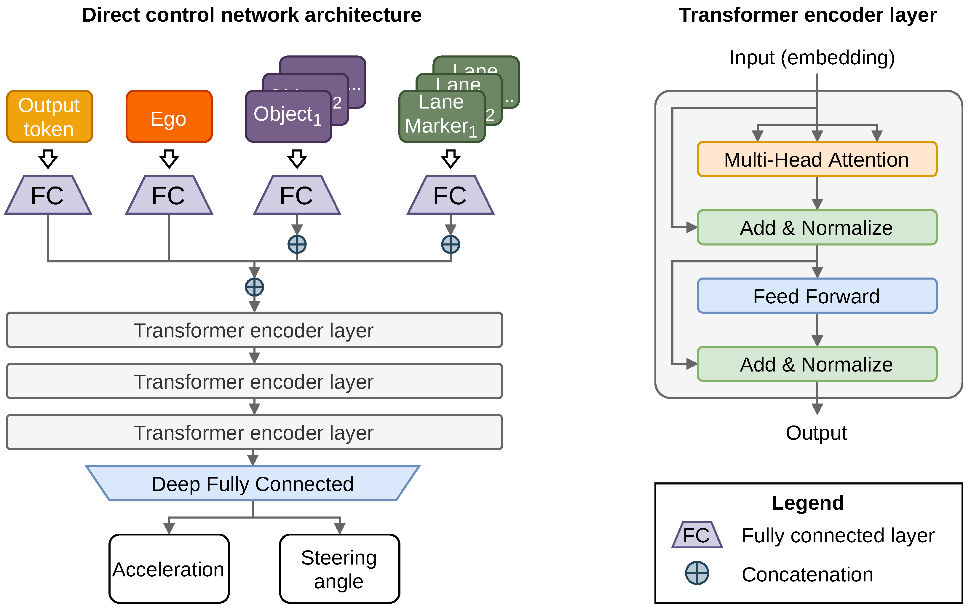
All of the observation values are normalized and processed by the transformer input model, which encodes them as shown in Figure 1 and passed to a deep fully connected network. The network returns output vector $a_{\varphi }({\mathbf{o}}_{\mathrm{ego}},{\mathbf{o}}_{\mathrm{obj}},{\mathbf{o}}_{\mathrm{lm}})={[a_{\mathrm{acc}},a_{\mathrm{steer}}]}^T$ of values ranged $[-1,1]$ that control the acceleration and steering angle of the ego vehicle. Both values are scaled by calibration parameters $p_{a_{\mathrm{acc}}},p_{a_{\mathrm{steer}}}$ accordingly.

3.3. Rewards

The control policy described in the previous section is trained with a PPO algorithm with a reward function composed of several terms listed below.

• Speed limit execution calculated at each step as a ratio of ego’s current velocity to a current speed limit, multiplied by a factor $r_{\mathrm{speed}\_\mathrm{limit}}$.
• Action values, specifically a squared acceleration and squared steering angle values, scaled by factors $r_{\mathrm{acc}}$ and $r_{\mathrm{steer}}$ respectively.
• Lane centering defined as a current distance of the ego vehicle’s center from the lane center multiplied by a factor $r_{\mathrm{centering}}$.
• Time To Collision calculated as a time at which a collision between the ego and another road user would collide if neither of them would change their current longitudinal acceleration nor lateral position. If constant accelerations would not lead to a collision or the time to collision is lower than $r_{\mathrm{ttc}\_\max }$, the value for this reward component is set to 0, otherwise, TTC scaled by $r_{\mathrm{TTC}}$ factor is assigned.
• Terminal states reward component assigned in events of a collision between the ego and other road user or a road barrier and exceeding the speed limit by $10\mathrm{m}/\mathrm{s}$ or more.

3.4. Training Setup

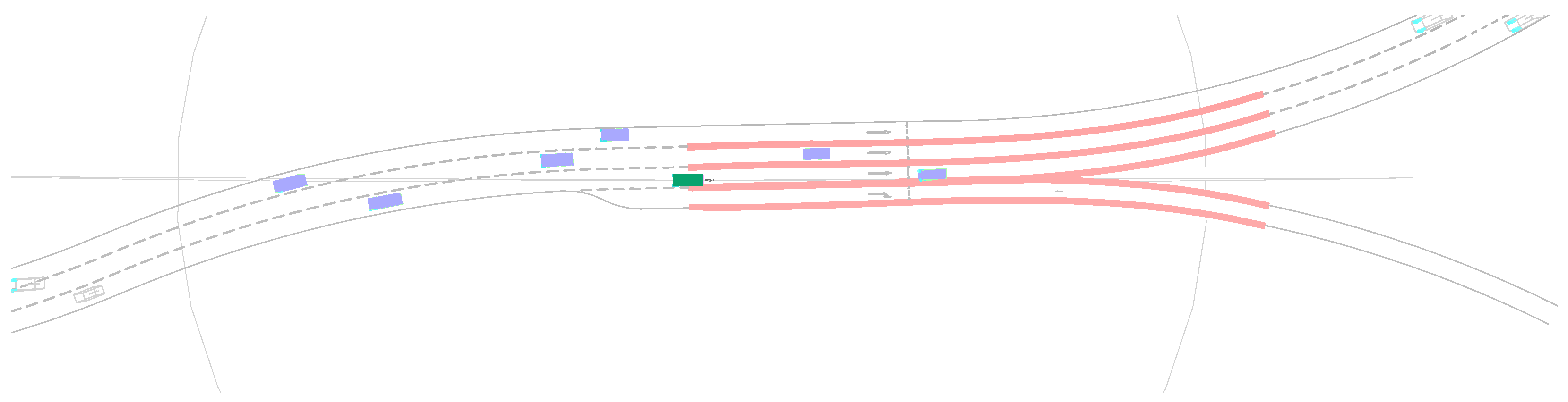
The experimental setup used for the evaluation of the proposed methods consisted of the simulation environment representing a randomly-generated multiple-lane highway featuring merge-in lanes, exit lanes, and vehicle traffic of varied density (see Figure 2). The movement of the road users (except for the ego vehicle) has been governed by a proprietary simulation package TrafficAI with rule-based semi-random driving policies. Simulation has been updated in 0.05 s timesteps, with the ego’s control values updated at every two steps. The direct control policy described in a previous chapter was trained for roughly 24 h in a distributed computing setup with 100 simulation threads used for data collection.

4. Evaluation Setup

Evaluation of the proposed sensor models in the context of the Reinforcement Learning policy training task comes with several challenges. Since one of the main purposes of the RL-based driving policy is to govern interactions with other road users, the end-to-end evaluation typically requires a closed-loop setup. On-road testing, while most informative, poses severe collision risks due to inherent limitations of the policy trained in a ground-truth environment.

Certain open-loop tests could be performed to assess policy’s robustness, e.g, through the comparison of the actions chosen based on ground-truth data to the sensor-based actions, similarly to Probably Approximate Correct sensing system evaluation methodology described in [24]. Since models proposed in this article focus mostly on object-level radar-based sensing systems, this method is unfortunately not feasible due to the lack of open datasets with radar-based object detection and tracking outputs.

Considering these limitations, I evaluate the policy’s performance in two ways: through large-scale driving tests in the simulation environment, and in the distribution of pre-defined test scenarios. In order to provide an insight into the impact of the sensor model’s use in the training process on the end policy performance, an additional set of baseline sensor models (described in the next subsection) is introduced for testing and comparison purposes. Policies trained in environments with both types of sensor models (proposed and baseline), as well as in the ground-truth environment, are cross-tested in all three types of training environments.

4.1. Baseline Sensor Models

A set of baseline sensor models is used to evaluate the impact of the particular sensor model’s design on the end policy’s performance, as well as to enable comparison of the policy trained in the ground-truth environment to the policy trained with the proposed sensor model in a relatively independent experimental setup. Baseline models fulfill the following set of tasks:

• introduction of state estimation errors through the addition of Gaussian noise,
• limitation of the observed lane markers distance to a value drawn from a normal distribution,
• simulation of the false negative object detection errors by random assignment of the binary visibility flag at each timestep,
• simulation of the false positive object detections through the creation of single-timestep objects with normally distributed state values,
• disturbance of the observed lane markers geometry performed through adding the Gaussian noise to the coefficients of the lane markers polynomials.

The parameterization of the models is described in

Table A5. Parameters of baseline sensor models (G-SM).

Parameter	Value
Object position error covariance matrix	$\left[\begin{array}{cc}1.2& 0\\ 0& 0.7\end{array}\right]$
Velocity error variance	2.0
Object length error variance	0.5
Object length error lower limit	−1.0
Object width error variance	0.5
Object width error lower limit	−1.0
False positive detection probability 1	0.0575
False negative detection probability 2	0.1
Lane marker mean observed length	87.0
Lane marker observed length variance	5.0
Lane marker observed length upper limit	90.0
Lane marker coefficients errors covariance matrix	diag (0.005, 0.0005, 0.00005, 0.000005)

¹ Parameters of the false positive object detections are drawn from the same distributions as described in Table A1. ² Duration of the false negatives is fixed to a single timestep.

.

4.2. Test Scenarios

In order to acquire an in-depth understanding of how various error patterns impact the trained policies, they are additionally evaluated in a set of short test scenarios. Each scenario is defined by a set of parameters that are drawn from pre-defined distributions. This approach allows running evaluation over a large distribution of scenarios of a given type and gathering statistical information about the agents’ performance.

Test scenarios incorporate common error patterns such as late detection of a vehicle, state estimation errors, and false negative detection errors. Scenarios parameter distributions are defined in a way that makes scenarios relatively challenging, and the performance is evaluated by counting a fraction of scenarios that ended in a collision with other vehicles or a road barrier.

Each of the evaluated policies is tested in 100 sampled variants of each scenario class, providing an insight into agents’ robustness to different types of errors.

A detailed description of the test scenarios with the parameter distributions is provided in Appendix B.

4.3. Evaluated Policies

Training has been performed in three setups: one with the sensor models described in a previous chapter (denoted Ornstein–Uhlenbeck-based sensor models environment, or OU-SM), one with baseline sensor models (denoted Gaussian-based sensor models environment, or G-SM), and one with ground-truth data (GT environment). All three trainings were performed with identical values of training hyperparameters and simulation parameters, listed in

Table A4. Proximal Policy Optimization training hyperparameters.

Hyperparameter	Value
Train batch size	250,000
Minibatch size	5000
Num epochs	15
Discount ($\gamma$)	0.99
GAE parameter ($\lambda$)	0.95
Clipping parameter ($ϵ$)	0.3
KL coefficient	0
Entropy coefficient	0
VF coefficient	1.0

.

5. Results

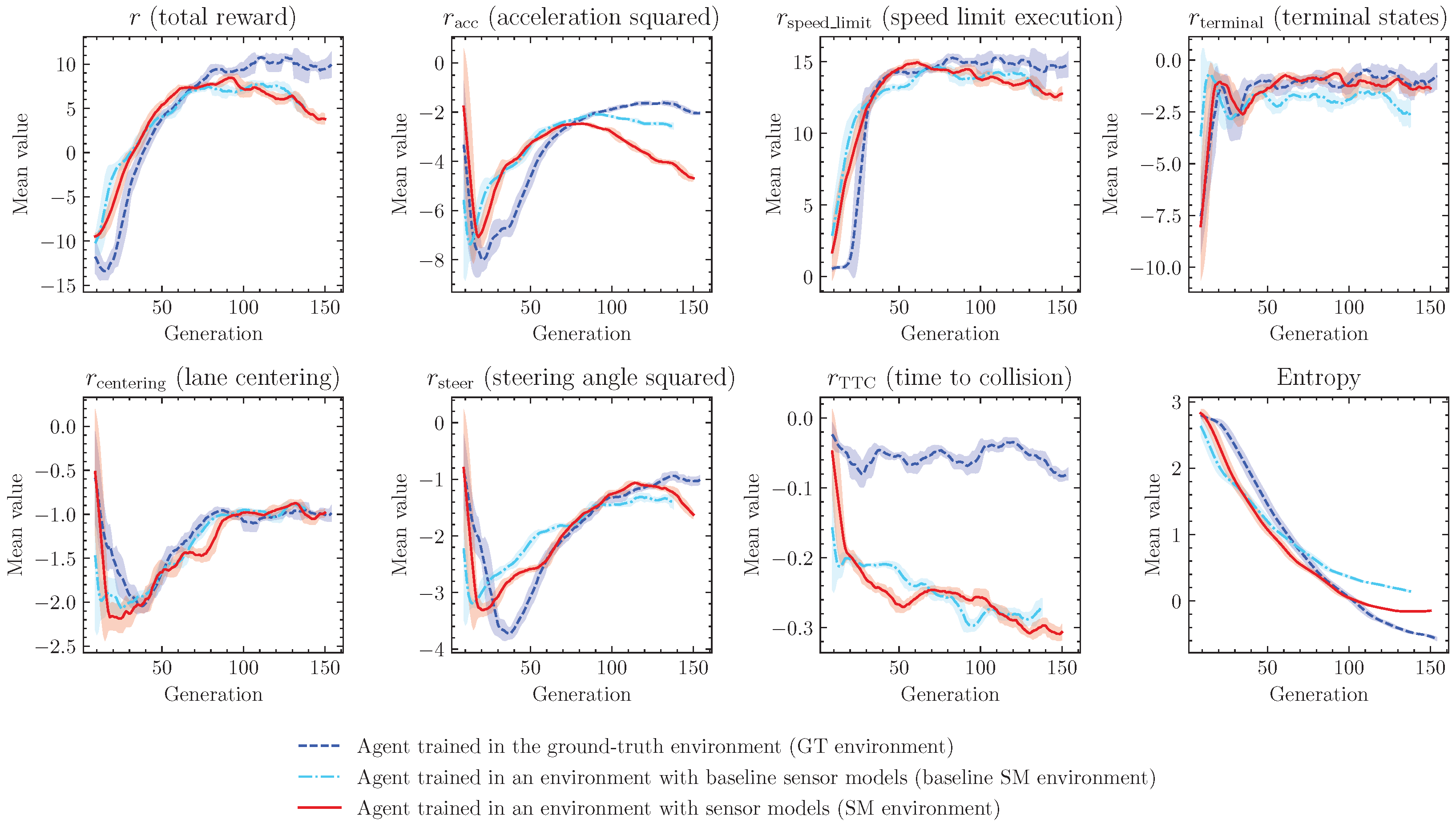
Progress of the training in all three environments (ground-truth (GT), with baseline Gaussian-based sensor models (G-SM), and with sensor models proposed in previous chapters (OU-SM)) is presented in Figure 3. In all cases, the training progressed in a similar manner, showing a rapid increase in the terminal states’ reward value, followed by a fast increase in speed limit execution value, and a long phase of entropy decrease, resulting in a slow improvement of rewards related to steering angle and acceleration. The final values of all rewards are relatively close, with a noticeable advantage of the agent in the GT environment.

Evaluation of the trained agents was performed in the highway simulation environment by running 100 simulation episodes, terminated after a collision, or reaching 1000 simulation steps. The evaluation was performed in nine experimental setups, testing the performance of each of the agents (trained in GT environment, G-SM environment, and OU-SM environment) in each of the three training environments.

A set of Key Performance Indicators (KPIs) was calculated based on performed evaluations, including the mean length of the episode (while the maximum length is 1000 simulation steps, an episode can be terminated early due to collisions), the average number of heavy braking events (defined as situations in which the agent applies acceleration below 2.0 $\frac{\mathrm{m}}{\mathrm{s}}$), a fraction of episodes failed (terminated before reaching 1000 simulation steps due to collision with other vehicles or road barrier), and other indicators. A full list of the KPIs with the values evaluated in all experimental setups is presented in

Table 1. Key Performance Indicators for evaluated agents. The table summarizes the evaluation of three driving policies (GT agent - policy trained in the ground-truth environment, G-SM agent - policy trained in the environment with baseline sensor models based on Gaussian noise, and OU-SM agent, which was trained in an environment with sensor models proposed in previous chapters). Each policy was evaluated in three simulation environments - with GT data, with G-SM setup, and with OU-SM setup.

	GT Agent			G-SM Agent			OU-SM Agent
Performance Indicator	in GT env	in G-SM env	in OU-SM env	in GT env	in G-SM env	in OU-SM env	in GT env	in G-SM env	in OU-SM env
Mean episode length (sim steps)	977.4	716.8	291.5	925.8	927.2	804.0	907.6	941.8	910.8
Average speed [$\frac{\mathrm{m}}{\mathrm{s}}$]	27.6	27.9	26.0	29.1	29.4	29.0	26.0	26.2	27.1
Average abs steering angle [rad]	0.35	0.56	0.30	0.54	0.57	0.62	0.41	0.46	0.48
Average abs acceleration [$\frac{\mathrm{m}}{{\mathrm{s}}^2}$]	0.64	0.91	1.23	0.68	0.76	0.82	0.98	0.91	0.99
Heavy braking events	1.7	8.7	1.5	2.9	7.6	4.1	2.7	8.2	3.5
Fraction of episodes failed	0.03	0.48	0.84	0.04	0.07	0.27	0.03	0.02	0.03

.

Trained policies were additionally evaluated in a set of test scenarios described in Appendix B. Results of the evaluation are presented in

Table 2. Performance of the agents in test scenarios. Each agent was evaluated in each scenario type 100 times, where scenarios for each run were sampled from the distributions described in Appendix B. Performance in the table is measured by a fraction of sampled scenarios evaluations that ended in collisions (the lower the better).

Scenario Type	GT Agent	G-SM Agent	OU-SM Agent
A. Late detection of a slow-moving object in front, empty highway	0.16	0.23	0.06
B. A constant error of front object’s speed estimation	0.41	0.73	0.31
C. Normally distributed error of front object’s speed estimation	0.45	0.30	0.24
D. Normally distributed front object’s lateral position estimation error	0.26	0.37	0.12
E. Random occurrences of false negative detection errors of front object	0.12	0.14	0.06
F. Frequent false negative road markers detections	0.11	0.06	0.04

, with a performance expressed in a fraction of the scenario episodes that ended in a collision of the ego vehicle with a road barrier or other vehicle. Note that the parameters of the scenarios are drawn from random distributions, and a certain subset of scenarios may incorporate situations, in which a collision is unavoidable.

6. Discussion

An agent trained in the ground-truth (GT) environment achieves satisfactory performance in the randomly-generated GT evaluation episodes. The ego controlled by the trained policy reaches the speed limit in a smooth manner and is able to keep constant velocity on an empty road. The presence of the slower-moving vehicles results in an expected velocity decrease, where the agent adjusts its velocity to a vehicle in front of it, keeping a moderate distance from it. The agent typically moves near the lane center, sporadically performing a lane-change maneuver, e.g., when the front vehicle moves with a velocity significantly below the speed limit.

As shown in Table 1, evaluation in the environment with proposed sensor models (OU-SM environment) results in a significantly lowered performance. The presence of the sensor errors results in increased absolute accelerations, due to frequently observed late sudden breaking, and lowered overall speed. The most significant issue, however, is related to collisions with the road barriers, reflected in significantly lowered mean episode length. Analysis of the evaluation episodes shows three major situations in which the agent is prone to road barrier collisions, listed below.

• Lane geometry errors in absence of nearby vehicles. Even minor geometry errors frequently result in situations, where the agent drives close to the side of the road, triggering the road barrier collision terminal state due to touching the road barrier.
• Late detection of the vehicle in front. Since the situation in which a slow-moving vehicle appears in close proximity to the ego cannot be observed in the ground-truth environment, where the vehicle is observed as soon as it enters the detection area, the driving policy is not trained to handle such situations properly. Late detection typically results in a severe steering maneuver in an attempt to avoid the collision. Excessive control values applied to achieve this however result in a sharp turn, causing a severe collision with a road barrier.
• False-positive object detections. False positives appearing in front of the ego vehicle result in behaviors similar to the ones described in a previous point. The ego attempts to avoid the collision through a severe steering maneuver, crashing into a road barrier due to an excessively sharp turn. Interestingly, false-positive objects that appear outside the road (behind a road barrier) also seem to destabilize the control policy - often triggering unexpected steering maneuvers that result in a collision.

An agent trained with an environment with baseline sensor models (G-SM) demonstrates significantly improved robustness to such issues, although it still does not achieve satisfactory performance in terms of collision avoidance, with $27\%$ episodes in OU-SM environment ending prematurely due to a collision.

The use of the sensor models in the training alleviates described issues. The performance of the driving policy trained this way is slightly lower compared to the policy trained in GT and G-SM environments, likely due to more cautious behaviors, such as keeping larger distances from other vehicles. The overall behavior of the OU-SM agent however remains similar to the GT and G-SM agents evaluated in their respective training environments. Interestingly, the OU-SM policy tested in the G-SM environment slightly exceeds the G-SM policy’s performance in aspects related to collision avoidance. This may be due to more cautious behaviors learned in a response to long-lasting time-correlated errors observed in the OU-SM environment.

Analysis of the test scenarios evaluation results leads to similar conclusions as the evaluation in the highway driving environments. The OU-SM agent demonstrates increased robustness to common error patterns, such as late detections and state estimation errors, compared to the policies trained in GT and G-SM environments.

The difference in the performance is especially visible in cases of long-lasting errors, such as constant velocity estimation error present in Scenario B. The presence of time-correlated state estimation errors in the OU-SM environment likely prevented the policy from overly relying on a small subset of observed environmental features, and the resulting agent seems to perform reasonably well even if one of the state parameters is severely disturbed.

Interestingly, in several test scenarios agents trained in the GT environment achieved better performance compared to the G-SM environment. This may be caused by the G-SM policy’s tendency to avoid severe actions. Since the observation in G-SM frequently changes due to introduced state estimation noise, quick responses in form of large accelerations and/or steering angles would lead to significantly lower reward values in the training. The resulting policy is thus unable to quickly react to dangerous situations, leading to poor performance in challenging test scenarios. Both GT and OU-SM policies are able to react to sudden risks with more appropriately severe actions, executing harsh braking and steering maneuvers to avoid collisions.

7. Conclusions

Performed experiments allow drawing several conclusions related to the robustness of driving policies based on Reinforcement Learning and the impact of sensor errors on their training and performance.

Reinforcement Learning (RL) is often proposed as a candidate for driving policies training due to its good generalization capabilities and robustness to slight variations in the environment. Experiments performed in this study seem to partially confirm the generalization capabilities of RL-based policies, as the agent trained in the GT environment is able to navigate in the traffic environment, even if the observation is severely disturbed by the introduced sensor models. Nonetheless, the experiments with sensor models expose several safety hazards caused by the sim-to-real gap in the policies trained in GT environments, such as the tendency to overreact in events of late detection or false positive detection errors.

Relatively good performance of the agent trained in GT environments may result in a false sense of safety—so it is especially important to ensure the presence of the additional safety mechanisms and to extensively test all machine-learning-based driving policies in challenging environments. While the errors introduced in the SM environment in this study were severe enough to expose the hazards, realistic sensor errors observed in good weather and lighting conditions may not be sufficient to trigger safety-critical errors in the evaluation with real-world data. Possible ways to alleviate this issue include testing in various SM environments, or the use of automatically-generated adversarial test scenarios to ensure good coverage of edge cases [25].

High-level sensor models proposed in this publication may be utilized for both testing and training driving policies. Policy trained in the environment with the sensor models is able to achieve performance levels similar to ones trained in GT environments while providing robustness against false positive and false negative object detection errors, object and lane markers state estimation errors, as well as false negative lane markers detection errors.