Abstract
Human activity recognition (HAR) is a popular and challenging research topic driven by various applications. Deep learning methods have been used to improve HAR models’ accuracy and efficiency. However, this kind of method has a lot of manually adjusted parameters, which cost researchers a lot of time to train and test. So, it is challenging to design a suitable model. In this paper, we propose HARNAS, an efficient approach for automatic architecture search for HAR. Inspired by the popular multi-objective evolutionary algorithm, which has a strong capability in solving problems with multiple conflicting objectives, we set weighted f1-score, flops, and the number of parameters as objects. Furthermore, we use a surrogate model to select models with a high score from the large candidate set. Moreover, the chosen models are added to the training set of the surrogate model, which makes the surrogate model update along the search process. Our method avoids manually designing the network structure, and the experiment results demonstrate that it can reduce 40% training costs on both time and computing resources on the OPPORTUNITY dataset and 75% on the UniMiB-SHAR dataset. Additionally, we also prove the portability of the trained surrogate model and HAR model by transferring them from the training dataset to a new dataset.
1. Introduction
HAR is an essential task in computer vision, which aims at analyzing the long-term behavior pattern and recognizing the specific type of behavior from the input data [1]. It has been widely used in virtual reality [2], automatic driving [3], and smart home environment monitoring [4]. Especially with the significant rise in the population over 65, the personal expenditure on medical service and long-term care are increasing sharply due to the awakening of health consciousness [5], HAR also plays a vital role in helping the elderly living alone, and the youth who need medical care [6].
Traditional HAR uses video data to identify human activity [7,8,9], which extracts Red-Green-Blue (RGB) and depth feature first, then sends these features into an end-to-end network, such as CNN [10], LSTM [11], etc. However, due to difficulties in camera deployment and the noise in video data, there is still a long way to go for large-scale commercial applications. As wearable devices and smartphones become more and more popular these days, a mass of human activity data can be easily accessed, and various sensor devices have been integrated into our lives (accelerators, gyroscopes, magnetometers, etc.), they are small in size and independent of the environmental setting, which makes human motion data including velocity, acceleration, and position offset can be generated, recorded or even calculated easily. In addition, their characteristics such as low price, low energy consumption, and high capability of data processing are valuable from an engineering perspective [12]. In this paper, we concentrate on the sensor-based HAR method and find a better solution to build a high accuracy and low consumption model.
Network designing is vital in a deep learning task. Networks, such as Resnet [13], Vggnet [14], and Densenet [15], are designed artificially by experts who have rich experience. Beyond all doubt, they have excellent performance, but also have a large number of parameters, which means the model needs much data to train. Besides, the model designing process heavily depends on prior knowledge, which is difficult for new researchers. A new approach is urgently needed. The successful application of NAS in deep learning helps researchers save both time and resources [16], and a model can be designed efficiently by defining a search space and a search algorithm. Furthermore, NAS’s structures always perform better than the manually designed ones.
Unlike the typical image classification tasks, the HAR task needs to extract both spatial and temporal features, and the models become heavier. To find an optimal set of parameters for a model, researchers need to repeat the experiments several times to adjust the parameters, which causes a severe waste of time and computing resources. NAS-based methods can automatically find the optimal network structure, which liberates the labor force. However, learning the optimal parameters of the network still costs iterations of stochastic gradient descent, and the computing load can reach hundreds of GPU-days [17]. Therefore, existing approaches primarily focus on mitigating the computational overhead, especially the SGD-based weight optimization [18,19,20]. Seeking to extrapolate rather than interpolate the performance of the architecture using surrogates is also an effective way to save resources. Furthermore, HAR models are always deployed in edge devices, which require a low-latency network to create a better user experience. So, we choose to use multi-objective NAS to focus on not only the accuracy of the HAR model but also its size of it.
This paper focuses on the recognition of human action based on the multi-objective NAS with online surrogates. We combine CNN with LSTM as a search space to extract both spatial and temporal features. The former can process the long-term features and avoid gradient vanishing by a gating mechanism, while the latter can extract different feature patterns by different convolutional kernels. Additionally, to promote the economic and intensive utilization of resources, we pay special attention to finding a lightweight but accurate HAR model that can quickly adapt to different types of edge devices. The contributions of the proposed methods can be concluded as follows:
- (1)
- We propose an efficient NAS for HAR application. The proposed method significantly reduces the training cost using the surrogate model. Besides, we propose a CNN–LSTM-based model for search space, which uses CNN to extract the features of the data automatically and uses an LSTM neural network to classify the action into a specific category.
- (2)
- We add floating-point operations per second (FLOPs) and the number of parameters into the model as the second and third objectives. The objective function ensures the model has low computation and communication overhead, which can achieve excellent performance in resource-limited scenarios.
- (3)
- The portability of the proposed method is proved by migrating the models trained on the OPPORTUNITY dataset to the UniMiB-SHAR dataset. The experimental results show that the model obtained through the searched network and the surrogate model can be applied to data with different distributions, which is of great significance for practical application.
The rest of this paper is organized as follows. In Section 2, we summarize the previous works that are related to neural architecture search and human activity recognition. In Section 3, exact expressions are derived for the proposed NASHAR scheme. In Section 4, we introduce the experiment settings, including hyperparameter settings and experimental environment. In Section 5, the results of the experiment are analyzed, including the performance of the searched architectures and the surrogate models. Finally, the potential future development of NAS-based HAR is discussed in Section 6.
2. Literature Review and Background
2.1. Literature Review on NAS Theory and Applications
In recent years, deep learning has achieved great success in many fields, including computer vision (CV), natural language processing (NLP), and auto speech recognition (ASR). Compared to traditional machine learning methods, deep learning has a strong learning ability and can extract the feature automatically, which liberates manual labor. Because of its practicability, deep learning has become more and more popular in many tasks. However, the problem remains that even though network structures in many tasks have been well-designed and architecture modifications do result in significant gains in the performance of deep learning methods, the search for suitable architectures is still a time-consuming, arduous and error-prone task. In the past several years, with the development of hardware equipment, NAS has been regarded as a revolution in network structure designing and has also placed high hope on breaking through the limitation of manual designing.
Generally speaking, NAS is cast as a search problem over a set of strategies that define the structure of a neural network, aiming at finding an optimal network from search space by using the search strategy. The search strategy details how to explore the search space; reinforcement learning (RL) and EA, for example, are the top two used methods. Zoph et al. [17] first defined NAS as an RL problem, considering the explore procedure as actions selection. It uses RNN as a controller to select an appropriate structure from the search space and then tests the network in the validation set to get the accuracy, which is regarded as the reward. Subsequently, the agent continues to maximize the reward until convergence. For EA [21,22,23], a population is generated firstly, followed by selection, crossover, and mutation, which is carried on periodically until it obtains the optimal structure. The above traditional methods regard NAS as a bilevel optimization problem on both network structure and weight in discrete domains, which are computationally expensive and limit the number of architectures that can be explored. Specifically, Refs. [24,25] both perform standard training and validation of the architecture on the dataset, which cost a lot of time and prevent the large-scale use of NAS.
Currently, the optimization of NAS is an important research topic that can help users find the optimal network structure in less time. The emergence of DARTS [26] breaks a logjam. It transforms the network structure search into a continuous space optimization problem. Therefore, the gradient descent method can be used to solve the problem while selecting the candidates, which makes the search process more efficient. In addition, sequence optimization is another implementation of search strategies. Liu et al. [17] use a sequential model-based optimization (SMBO) algorithm to improve the complexity (depth) of the search space and uses the surrogate model to optimize the exploration process. Compared with the previous methods, this method has substantially reduced the computational resources required for NAS (from thousands to a few GPU days). More specifically, the computational complexity is reduced by about 88%, the number of models that need to be trained is reduced by about 80%, and the quality of the production is almost unchanged. Besides, strategies like Monte Carlo tree search (MCTS) [27] and Bayesian optimization [28] are also used.
The Performance estimation strategy is also essential. The candidate models are sampled and then trained to convergence to measure their performance on the specific task. The architecture that achieves the highest predictive performance on the validation set will be chosen. During the search, each evaluation of a candidate involves an expensive process of training and testing, which is computationally expensive and time-consuming. As mentioned above, the computational bottleneck of NAS is the training of each child model to convergence. Therefore, it is necessary to reduce the cost. The simplest way is to reduce the training time (the number of iterations), that is, to train the network on a subset of the training set or to reduce the number of layers of the network. Although these methods can speed up the evaluation process, they will inevitably introduce biases, which cause severe damage to the model performance, and even retain the low-performance model by mistake. Guo et al. [29] try to use a surrogate model to evaluate the performance of the generated candidates before testing on the validation set, and the model with poor performance will be discarded, thus significantly reducing the time-consuming on the premise of ensuring the accuracy.
We categorize methods for NAS according to three dimensions: search space, search strategy, and performance evaluation strategy (respectively corresponding to , , and in Table 1). The search space is a set of candidate network architectures. To save time and resources, we permanently reduce the search space with prior knowledge to simplify the search process. The search strategy means the specific method to find the optimal network structure. Performance evaluation strategy refers to the process of estimating the candidate network structure, which aims at discarding the poor candidates and selecting better models. In Table 1, we introduce three types of literature , , and . Refs. [26,30] are about the search space. Refs. [17,21,24,27,28,31,32,33] introduce the research on different search strategies. Refs. [17,22,29,34] are some innovate performance evaluation strategies.

Table 1.
Related work on NAS.
2.2. Literature Review on HAR Methods
Traditional HAR methods require complex handcrafted features, which make it hard to apply for practical tasks. They need to extract features such as shape [35], trajectory [36], optical flow, and local spatiotemporal interest points [37], specifically including static features such as contours and shapes, dynamic features such as optical flow or motion information, spatiotemporal features such as space-time cubes, and descriptive characteristics. Manual feature extraction is time-consuming and not flexible. When new data is available, researchers need to reanalyze the data and repeat the above process.
With the development of deep learning, automatic feature extraction has gradually become mainstream. Three main approaches are two-stream-based, Convolutional3D (C3D)-based, and CNN-LSTM-based methods.
The two-stream-based method focuses on extracting the optical flow feature, which represents the motion pattern of the human, and then fuses with the RGB feature to classify the input. Karen et al. [38] proposed a two-stream CNN architecture combined with a spatial and temporal network, both of which are trained on multi-frame dense optical flow and can achieve excellent performance. Tang et al. [39] use a two-stream network to predict human action and achieve impressive results in both short-term and long-term predictions. This kind of two-dimensional (2D) convolution can extract spatial features well, but rarely deals with temporal features. So, Ji et al. [40] extended the traditional 2D-CNN [41] to 3D-CNN, performing feature extraction in both the time dimension and space dimension, which means the feature maps among adjacent frames can interact during the convolution process. Guo et al. [42] employ 3D-CNN and statistic analysis algorithms to extract video and WiFi features, respectively, and propose a novel multi-modal learning approach for video and WiFi feature fusion. Although 3D-CNN grew dramatically to improve the recognition accuracy, it also increases the number of parameters. Therefore, new methods are urgently needed.
RNN-based models have also been widely used to exploit the short and long-term temporal dynamics for their powerful ability to model temporal dependencies. However, it has a severe short-term memory problem. Long-term data has little influence on subsequent data, even if it is essential. Thus, variants such as LSTM and gated recurrent unit (GRU) emerge to effectively retain long-term information, which can not only learn the reliability of the sequential input data, but also use the memory cell to adjust its effect. Many network structures combine CNN with RNN to extract both spatial and temporal features. Arvind et al. [43] propose a multi-task recurrent neural network architecture that uses inertial sensor data to segment and recognize activities and cycles, which outperforms or defines state-of-the-art HAR and cycle analysis using inertial sensors.
We divide the research of HAR into three categories, data enhancement, feature extraction, and model training, and collect related works in recent years, as shown in the Table 2, where denotes the studies on data enhancement as Refs. [44,45,46,47,48], denotes the studies on feature extraction as Refs. [48,49,50,51], and denotes the studies on spatio-temporal network design as Refs. [17,52,53,54,55].
Table 2.
Related work on HAR.
2.3. Background and Significance
This paper mainly proposes a model auto search method for HAR. The neural network model is a basic current action recognition method that can accurately classify data. However, for different data and application scenarios, the parameters and structure of the model usually need to be adjusted manually, which requires manual experience and is time-consuming. The business background of this paper is to solve the problem of automatic model construction of HAR tasks to achieve automatic model updating and reduce manual workload. NAS provides a method to search neural network models automatically, but it also has the problem of a time-consuming search. The method proposed in this paper first solves the model search problem on HAR tasks, dramatically improving the search efficiency and ensuring good migration performance. It has significant application value for HAR tasks.
3. Methology
In this section, we first introduce the network structure and the definition of search space. Then we present the search strategy and the surrogate models, which are used to optimize the search process. The overall search procedure is summarized in Figure 1 as follows.
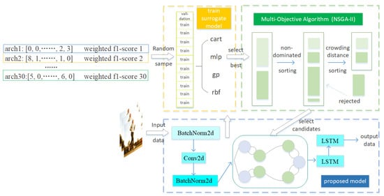
Figure 1.
The proposed HAR framework based on NAS with surrogate model and NSGA-II.
Firstly, the model randomly selects 30 different architectures as the initial training samples of surrogate models. Specially, we train four different types of surrogate models, including multi-layer perceptron (MLP) [57], classification and regression tree (CART)[58], radial basis function (RBF) [59] and Gaussian process (GP). The optimal surrogate model is chosen through 10 cross-validations. Secondly, we apply the surrogate model to the candidates generated by the multi-objective genetic algorithm, then individuals with excellent performance are picked and trained on the complete dataset. Finally, we add the selected individuals to the training set for the retraining of the surrogate models. We repeat the above process several times until the Pareto front is convergent.
3.1. Search Space
LSTM is commonly used in NLP tasks to extract relations among words, which has some similarities with extracting temporal features in HAR tasks. Additionally, to analyze the spatial features, we combine CNN with LSTM to design a high-precision but lightweight network. As advocated above, compared with the hand-craft method, NAS serves as a more appealing method for optimizing neural architectures to get a lightweight model. For the CNN part, we define a cell search space to be a set of basic operations where the input and output feature maps have two types of spatial resolution, which are proposed in DARTS [26]. Each cell consists of multiple blocks, and it can be regarded as a directed acyclic graph (DAG) with N nodes where N equals 5 in this paper. Each cell has two inputs and one output. The specific schematic diagram is shown in Figure 2. In the CNN module, the two inputs of the cell correspond to the output of the previous two layers. Specifically, the two types of cells are normal ones and reduction ones, and the difference between them is that the latter will reduce the height and width of the feature maps by half, 1/3, and 2/3 of the network. These searching cells will repeat over all the cells in the network topology level.
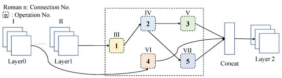
Figure 2.
Search operations and connections.
The blocks mentioned above contain three main operations, namely skip connect, convolution and pooling. Additionally, there are ten types of subcategory operations. The continuation strategy of these candidate operations between nodes can be expressed as follows:
where O denotes the operation set described in Table 3, while refers to the weight of operation o on directed edge from i to j . The discretization value of the mixing operation between node pairs can be depicted as follows:
Table 3.
Optional operations in search space.
All operations have the same stride equals 1. Moreover, proper padding is used to keep the size of the feature map the same. The details of optional operations of the search space are summarized in Table 3.
3.2. Search Strategy
The search strategy defines an algorithm to select individuals from the population to hybridize and generate new individuals. After mutating and screening, individuals with bad performance are eliminated and then a new population is generated. In this paper, we use NSGA-II [60] as the basic search strategy. NSGA-II is a kind of multi-objective EA, which is optimized from the algorithm NSGA-I [61]. Compared with the NSGA-I, NSGA-II, a more efficient and elitist search method, has some improvements, as follows: (1) It proposes a fast non-dominated sorting algorithm. (2) It uses congestion degree and congestion degree comparison operators to select candidates. (3) It applies the elite strategy to generate offspring. Multi-objective optimization purports that we must pay attention to two or more objectives when a task needs to be completed. For example, in the design of automobile body parts, it is required that the designed parts have great stiffness and lightweight, which is a two objective optimal problem with some conditional constraints, such as dimensional constraints and modal constraints. Multi-objective optimization can be described as follows:
where refers to different objective function, denotes constraint function and x represents the feasible region in the task.
As for details of NSGA-II, it is a fast non-dominated multi-objective optimization algorithm with elite retention, which is based on Pareto Optimality (PO). Based on natural selection and survival of the fittest, NSGA-II obtains the optimal target population through population cycle iteration. First, it randomly generates the initial population. Then, it uses the non-dominated sorting (NDS) method to select individuals. Finally, it sets a loop iteration through a multi-objective optimizer with crossover and mutation operations to find the final population. The process of the NSGA-II algorithm is described as Algorithm 1.
| Algorithm 1 General process of NSGA-II. |
Input: Populations P, number of generations g, offspring S, basic operations O, select operations , crossover operations , mutation operations Output: Final population
|
In this paper, weighted f1-score, FLOPs, and the number of parameters (PaNo) is used as the training objectives. The weighted f1-score denotes the recognition accuracy. FLOPs and PaNo indicate computing complexity. Generally, high accuracy always brings more computing complexity. With the widespread of smartphones and other edge devices, HAR models also need to be deployed on those devices with limited computing power. Therefore, we compromise accuracy and model complexity and choose the above indicators to measure the searched model in our HAR task.
3.3. Surrogate Model
Two main computing bottlenecks remain on the general NAS task. One is complete training, which usually takes several days with a multi-GPU server. The other is that many alternative network structures need to be evaluated, which consumes much time and computing resources before the Pareto front convergence. To overcome the above bottlenecks, we use a surrogate model to predict the weighted f1-score from integer strings that encode architectures, which is depicted in Figure 2, and select those with high scores to the new population. The specific process can be described as follows:
where denotes the accuracy value of model architecture, denotes the node coding matrix of NAS searched model structures and refers to the surrogate model to get the best surrogate model for each round adaptively. We use an adaptive switching (AS) selection mechanism, which firstly builds four types of surrogate models in each iteration, namely MLP, CART, RBF, GP, and then selects the best one by cross-validation. It is worth mentioning that the surrogate model is trained and set online. Compared with the previous methods, which use offline methods to construct the surrogate model, means the surrogate model is trained completely before the search process and without an update, of which the timeliness performance is low and the effects are greatly influenced by the initial random sample. By using an online surrogate model training strategy, the selected models are added to the training set of the surrogate models. Therefore, each update of the population is also accompanied by an update of the training set of the surrogate model. By using the surrogate model, the searching procedure can be lighter and fast with almost constant accuracy.
3.4. Proposed Approach
In our proposed HARNAS method, we used NSGA-II as the multi-objective optimization and some simple methods as the surrogate model. The model is categorized into five parts that give a detailed account in Figure 3. They are the initial layer, pre-select layer, optimization layer, output layer, and objective task layer.
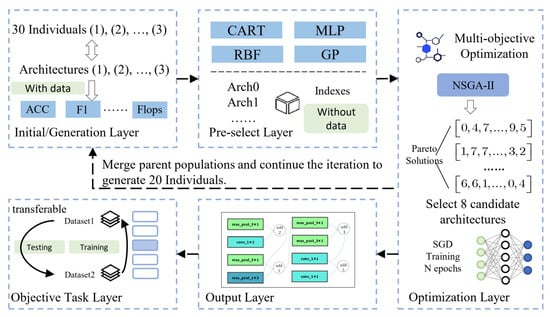
Figure 3.
The detailed approach and experiment description for HARNAS.
In order to construct the surrogate model, we first randomly sample 30 alternative models and obtain the weighted f1-score of these candidates by thoroughly training on the dataset in the initial layer. Then, we encode these candidate models into integers as the input features, and weighted f1-score, FLOPs, and PaNo serve as labels while training surrogate models in the pre-select layer. After that, the surrogate model with the best cross-validation result is obtained. Next, in each iteration, 20 new individuals are generated through genetics, crossover, and mutation. The surrogate model infers the weighted f1-scores of these 20 individuals and selects the top eight of them as the new individuals of the population in the optimization layer. Then, these new individuals are evaluated without deviation by the genetic algorithm and are added to the training set of the surrogate model before the next iteration. The surrogate models are reupdated each round with the population iterates. Especially as the number of samples increases and individuals tend to the Pareto plane, the prediction performance of the surrogate model increases. Repeat the above process. We can finally obtain a convergent Pareto plane in the output layer. Then, we can choose to use it in downstream tasks.
4. Experiments
4.1. Datasets Description
There are many public datasets for HAR tasks, such as OPPORTUNITY [62], UniMiB-SHAR [63], J-HMDB [64] and Event-version UCF-11 [65]. Considering that low-noise and rich-category data can maximize the potential of the model, we use sensor data to validate our model, which contains less noise compared with RGB ones.
Dataset OPPORTUNITY: This dataset is collected by installing wearable devices, including seven inertial measurement units, twelve 3D acceleration sensors, and four 3D localization devices on the upper body (buttocks and legs) of four volunteers to capture their seventeen daily activities, which contains explicitly getting up, drinking coffee, eating a sandwich, cleaning the table, etc. All the activity recognition environments have been designed to generate many activity primitives, yet in a realistic manner. For each subject, six different runs were recorded. Five of them are called activity of daily living (ADL), while the remaining one, a drill run, was designed to generate many activity instances. The ADL run consists of temporally unfolding situations, which contain a large number of action primitives that occur. We trained our model on the ADL of the first and fourth subjects, as well as ADL1, and ADL2 of subject 2 and subject 3, and we evaluated the classification performance of the ADL4 and ADL5 of subject 2 and subject 3. The ADL3 dataset of subject 2 and subject 3 is left for validation.
Dataset UniMiB-SHAR: This dataset of acceleration samples was collected by Android smartphones. It equips with a Bosh BMA220 three-axis low-gravity acceleration sensor and can measure the acceleration on three vertical axes simultaneously. The dataset contains 11,771 human activities and falling samples from 30 subjects, ranging from 18 to 60 years old. During the data collection, the subjects were asked to put their smartphones in their front trouser pockets: half of the time in the left trouser pocket, and the rest in the right trouser pocket. According to different behaviors, the samples are divided into 17 fine-grained categories and 2 coarse-grained categories: one sample contains 9 activities of daily living (ADL), and the other has 8 types of falls. We used 10-fold cross-validation based on the predecessors, which means that all data are randomly divided into 10 parts, each of which is used as the test set in turn, and the remaining 9 parts are used as the training set. Then, we recorded 10 rounds of test results and took the average.
4.2. Data Processing
Before model training, it is necessary to pretreat data to ensure effectiveness. To avoid the missing data causing an unknown impact on the model training, we use linear interpolation to complete the data. Linear interpolation is the most convenient method to retain as much data information as possible. Other effective strategies can also be conducted here to increase and complete the data processing (e.g., synthetic minority oversampling technique (SMOTE), nearest neighbor interpolation, bilinear interpolation, etc.). Additionally, we treat each sensor axis as a separate channel and generate an input of 113 channels. As for data extraction, we first extract frames by sliding a fixed length. T denotes the size of the time window, and S represents the sliding stride. Each frame is built as a data matrix in the shape of T*S, of which the channel size is 113. For OPPORTUNITY, we use a time window of 2 s, and the T is selected as 64, and S is 3. For UniMiB-SHAR, we use a time window of 3 s, and T is designed as 151 and S is 3, which is similar to the settings in [66].
4.3. Evaluation Indexes
As depicted in Section 3.2, three indexes are selected as the multi-objectives. Weighted f1-score, FLOPs, and PaNo are expressed as , and . is calculated to evaluate the performance of the model. and are computed to test the complexity of the model. Weighted f1-score (): To evaluate the effect of classification results, we choose the weighted f1-score as the index, performing a weighted average of the f1-score of each category, according to the number of samples for each label. This alters "macro" to account for label imbalance, and it can result in an f1-score that is not between precision and recall. The confusion matrix is shown in Table 4.
Table 4.
Confusion matrix.
TP refers to the number of samples that are positive and also predicted to be positive with , FP refers to the number of samples that are negative but predicted to be positive with , FN refers to the number of samples that are actually positive but predicted to be negative with , and TN refers to the number of samples that are actually negative and predicted to be the negative class with .
According to these indexes, we can calculate the recall and precision. Recall refers to the ratio of the positive samples that are correctly predicted, while precision focuses on the part that is predicted to be a positive sample. These evaluation indexes are calculated as follows:
where M represents the total number of classes. , which represents the sample proportion of corresponding class labels. i denotes the data category in the dataset. Floating-point operations per second (FLOPs): FLOPs is the abbreviation of floating-point operations, which means the amount of floating point operations. It is usually used to measure the complexity of the model. The specific formulation in the convolutional layer and fully connected (FC) layer are as follows:
where and refer to FLOPs of convolutional layer and FC layer, is the input channel, is the convolutional kernel size, is the output map height, is the output map width, is the output channel, is the input neuron numbers and is the output neuron numbers. The number of parameters (PaNo): It refers to the size of the model, which has nothing to do with the input size and only describes the memory required by the model itself. The difference between the number of parameters and the FLOPs is that the latter refers to the number of operations including additions, subtractions, multiplications, and divisions in the actual process, which is related to the input.
Model Training Details
The proposed model is implemented using Python combined with the PyTorch library on a single NVIDIA 1080Ti GPU. Data processing, model training, and testing are all in the environment of Ubuntu 16.04, RTX 1080Ti*1, Cuda10.1, Python3.7.7, and PyTorch1.2.0.
The setting of hyperparameters is crucial. We first weigh up both efficiency and accuracy and finally choose 30 randomly sampled architectures as the initial training set of the surrogate model. Then, to prevent the model from over-fitting, the searched layers (number of cells) are set to 1, and the blocks (number of blocks in a cell) are set to 5. The population generates 40 new individuals each round, and then 8 optimal individuals are selected from them based on the latest surrogate model and iterates the above process for 10 rounds. As for model optimization, the batch size is set to 128. The stochastic gradient descent algorithm and cross-entropy are used for parameter optimization, and cosine annealing is used to adjust the learning rate. Each model trains for 25 rounds before the parameter converges.
5. Results and Discussion
In this section, we evaluate the weighted f1-score and the search efficiency of the obtained architectures on OPPORTUNITY and UniMiB-SHAR. Additionally, to increase network utilization, we make reusability one of our goals.
5.1. Performance of the Searched Architecture
Table 5 shows the HAR performance on two datasets of the proposed HAR-NAS method, which also lists several comparable basic methods and previous methods to demonstrate the effectiveness of our method.
Table 5.
Performance of comparative methods and the proposed NAS model on datasets OPPORTUNITY and UniMiB-SHAR.
We present a survey of different approaches toward the goal of higher performance on these two datasets as shown in Table 5. CNN and RNN-based models are widely used in HAR task, among the methods on the OPPORTUNITY dataset, the best accuracy is 91.29, the best micro-f1 score is 70.40 and the best weighted-f1 score is 92.07, while the models searched by our method achieve the state-of-the-art performance that the accuracy reaches 91.41, the micro-f1 score reaches 68.87 and the weighted f1-score reaches 92.09. Similarly, these indexes in the UniMiB-SHAR dataset are 75.52, 64.47, and 76.10, respectively, each of which is better than the performance of the existing methods. Additionally, we also present experimental studies on accuracy vs. efficiency trade-offs. Table 6 shows the parameter settings of the above models.
Table 6.
Parameter settings of comparative experiments on OPPORTUNITY and UniMiB-SHAR.
Pareto fronts are usually calculated by turning the multi-objective optimization problem into a sequence of single-objective optimization problems or exploiting evolutionary methods. A set of candidate solutions gradually evolve into the Pareto set. In multi-objective tasks, conflicts and incomparability always exist among different objectives, which means the better the performance of an objective, the worse the performance of other objectives, and the solutions are called non-dominant solutions or Pareto solutions. The set of the optimal solution is called the Pareto optimal set, and the surface formed by the set with three objectives in space is called the Pareto frontier surface. In the experiment, we set the multi-objective to be an error index (weighted f1-score), FLOPs, and the number of parameters. Figure 4 shows the Pareto fronts on the datasets. Besides, to analyze in detail, we also draw the relationships between every two objectives of the total three objectives on the two datasets.
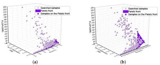
Figure 4.
Pareto fronts output in the experiment process.(a) Pareto front on OPPORTUNITY. (b) Pareto front on UniMiB-SHAR.
Figure 5 and Figure 6 draw the relations between objectives on the two datasets, which show that the individuals searched eventually tend to converge on the coordinate axis, that is the Pareto front.
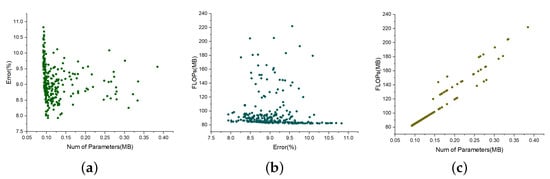
Figure 5.
The pairwise relationships of three objectives on dataset OPPORTUNITY. (a) Change relation between number of parameters and error. (b) Change relation between error and FLOPs. (c) Change relation between number of parameters and FLOPs.
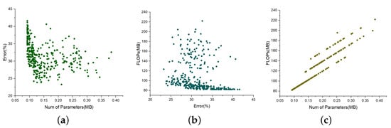
Figure 6.
The pairwise relationships of three objectives on UniMiB-SHAR. (a) Change relation between number of parameters and error. (b) Change relation between error and FLOPs. (c) Change relation between number of parameters and FLOPs.
In our task, the initial channel of the model is also a searchable parameter. As shown in Figure 7 below, we set the initial channel number to be 40, 48, 56, and 64, and search for 30 rounds, then use a box chart to make a visual analysis. We conclude that the larger the initial channel number, the relatively larger the parameters and FLOPs are, while the relationship is not strictly linear. In addition, it can also be seen that there is no apparent difference between the error rate of the selected models under these four different initial channels. That is to say, a complex model is not necessarily needed to improve recognition accuracy.
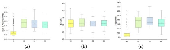
Figure 7.
The population searched on UniMiB-SHAR based on the tri-objectives search objective.(a) Number of Parametres. (b) Error. (c) FLOPs.
5.2. Performance of the Surrogate Predictors
The surrogate model greatly reduces the number of models that need to be completely trained by estimating the accuracy of the newly generated individuals, thereby solving the problem of unbearable time-consuming general NAS methods. Specifically, we train four different surrogate models each time and select the best one according to the Kendall-tau (TAU) distance [72], the correlation coefficient between the prediction and target. As shown in Figure 8 below, the adaptive method is much better than using just one type of surrogate model.
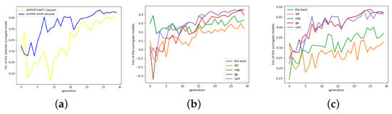
Figure 8.
TAU of the different surrogate models on OPPORTUNITY and UniMiB-SHAR. (a) The selected surrogate model on two datasets. (b) OPPORTUNITY. (c) UniMiB-SHAR.
Figure 8a is the TAU of the optimal surrogate model on the two data sets. It is shown that TAU oscillates along the whole process while still gradually tending to converge to a stable value. Figure 8b,c are the TAU of each surrogate model and the optimal surrogate model on OPPORTUNITY. We comprehensively consider the mean and variance of TAU during the entire 30-round iteration process, that is, we do not simply choose the model of the maximum TAU, but also consider the stability of the model.
5.3. Search Efficiency
To compare the search efficiency of our surrogate-based HARNAS method, we take the weighted f1-score as the index and compare the consumed time as well as the needed computing resource, which can be quantified to be the number of models that need to be trained along the whole process, and the fewer models need to be trained, the fewer resources to be consumed.
As shown in Table 7, for OPPORTUNITY, when the weighted f1-score of the general NAS method reaches 92.17, the number of models that need to be trained is 200. Compared with the NAS method using surrogate models, when the weighted f1-score reaches nearly the same level of 92.09, the number of models that need to be trained is 120, which is 1.67 times less than the general NAS method. Similarly, for UniMiB-SHAR when the weighted f1-score of the general NAS method reaches the best 75.64, the number of models that need to be trained is 100. Compared with the NAS method using surrogate models, when the weighted f1-score is best of 76.12, the number of models that need to be trained is 24, which is 4.17 times less than the general NAS method.
Table 7.
Efficiency comparison between the NAS model with surrogate model or not.
In addition to reducing the number of models that need to be trained and improving the training speed of the model while reaching roughly the same index as a general NAS method, we also compared the FLOPs and the parameters of these two indicators. On OPPORTUNITY, while reaching the same weighted f1-score, the FLOPs of the model searched by the surrogate-based NAS method are 1.22 times less than the general one, and the number of the parameters is 1.48 times less. For the UniMiB SHAR dataset, these two numbers are 2.54 and 1.66, respectively.
Our method can achieve better results in the multi-objective task, including accuracy, parameter amount, and FLOPs. We draw some of the architectures on the Pareto front of UniMiB-SHAR as Figure 9. As shown below, the input data is firstly operated by ReLUConvBN. The structure in the rectangular box is obtained by NAS search. The small rectangular boxes are the elements listed in Table 3. The hollow circle represents the summation operation. After the spatial feature is extracted through the NAS-searched structure, the spatial features are extracted by bi-LSTM, and finally, through the FC, the predicted output result is obtained.
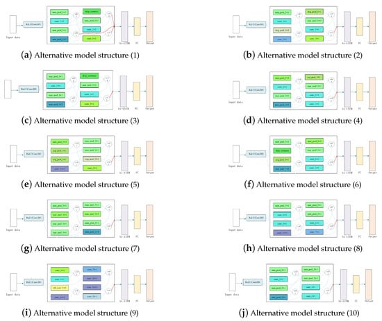
Figure 9.
Set of network models searched on the Pareto frontier of UniMiB-SHAR.
5.4. Transferring from OPPORTUNITY to UniMiB-SHAR
It is a common practice that models searched on one dataset need to be transferred to the other datasets or tasks dual to the limited resource. To test the transferability of our searched model and surrogate models, we transfer the model with the lowest error rate and its surrogate models from OPPORTUNITY to UniMiB-SHAR.
(1) Reusability of the Surrogate Model
Dealing with the same problem on different datasets will significantly save both time and computing resources if the trained surrogate model can be reused, and we can be searched for models directly without repeating the online surrogate training process.
We select the surrogate model of the model that achieves the best results in OPPORTUNITY to be directly used as the surrogate model on UniMiB-SHAR and use the offline method, that is, the searched individuals are not added to the training set of the surrogate model, and this model is reused throughout the whole search process. We compared the weighted f1-score with the method using general NAS methods. The results are shown in the following Table 8.
Table 8.
Reusability of the surrogate model.
As shown in Table 8, the general NAS methods can reach a weighted f1-score of 75.64, slightly lower than the method using the new surrogate model. Still, it is similar to the old surrogate-based method, which is trained from OPPORTUNITY. To improve the performance of the old surrogate model, we retain the surrogate model online, that is, each round of searching on UniMiB-SHAR uses the updated surrogate model. As seen above, when the HAR models reach nearly the same weighted f1-score, the parameter amount and FLOPs of the models searched by the migrated online-surrogate model are much smaller than those searched by general NAS methods, and the number of models needs to be trained to obtain the optimal architecture is also reduced by 12. Similarly, we compared the model directly using the old surrogate model and offline training. Our method obtains the optimal model of convergence in less time, while the performance is slightly lower than the model of online training.
(2) Reusability of the Searched Model
Similar to (1), we directly transfer the optimal model searched on OPPORTUNITY to UniMiB-SHAR, and the weighted f1-score reaches 72.1%, which is only slightly lower than the best result searched by the general NAS. In some practical applications, what we often pursue is not the highest accuracy, but the deployment ability of the model. The method that directly migrates models from one dataset to another significantly improves the engineering efficiency and iteration capability of edge applications.
6. Conclusions
In this paper, we apply the surrogate-based NAS method to the HAR task, adopt an adaptive method to flexibly select the optimal surrogate model, and continuously improve its performance through online training. This method solves the unbearable time-consuming problem and provides a new solution for traditional NAS methods. Using efficient NAS allows our method to deliver strong empirical performances while using much fewer GPU hours than existing automatic model design approaches, and notably, 4× less expensive than standard NAS on the premise of achieving the same classification accuracy. Besides, the searched model and surrogate model perform well on the new dataset, which shows a strong ability of reusability.
The proposed method will help people build HAR frameworks conveniently and efficiently. This work has specific significance for further improving the construction efficiency, migration, and generalization of HAR models in the future. In the field of NAS and HAR, we will try in-depth research on lightweight models to help them deploy on-edge devices. Besides, considering the layers in deep neural networks are not isolated, the traditional rule-based pruning strategies are not optimal and cannot be migrated from one model to another, so we will try to use reinforcement learning, for example, to further improve search efficiency.
Author Contributions
Conceptualization, M.H. and X.W.; data curation, Y.Z.; methodology, M.H., X.W. and L.Y.; supervision, M.H., X.W. and L.Y.; writing-original draft, M.H. and Y.Z.; writing review and editing, M.H., X.W., L.Y., H.W. and Y.Z. All authors have read and agreed to the published version of the manuscript.
Funding
This work was supported by the National Natural Science Foundation of China (Grant No. 62071056) and the National Natural Science Foundation of China (Grant No. 61871046).
Data Availability Statement
The datasets used in this paper are available online, and they are also available from the corresponding author upon request.
Conflicts of Interest
The authors declare no conflict of interest.
References
- Beddiar, D.R.; Nini, B.; Sabokrou, M.; Hadid, A. Vision-based human activity recognition: A survey. Multimed. Tools Appl. 2020, 79, 30509–30555. [Google Scholar] [CrossRef]
- Pareek, P.; Thakkar, A. A survey on video-based human action recognition: Recent updates, datasets, challenges, and applications. Artif. Intell. Rev. 2021, 54, 2259–2322. [Google Scholar] [CrossRef]
- Braunagel, C.; Kasneci, E.; Stolzmann, W.; Rosenstiel, W. Driver-activity recognition in the context of conditionally autonomous driving. In Proceedings of the 2015 IEEE 18th International Conference on Intelligent Transportation Systems, Gran Canaria, Spain, 15–18 September 2015; IEEE: Piscataway, NJ, USA, 2015; pp. 1652–1657. [Google Scholar]
- Civitarese, G. Human Activity Recognition in Smart-Home Environments for Health-Care Applications. In Proceedings of the IEEE International Conference on Pervasive Computing and Communications Workshops 2019, Kyoto, Japan, 11–15 March 2019; p. 1. [Google Scholar]
- Sarngadharan, D.; Rajeesh, C.; Nandu, K. Human Agency, Social Structure and Forming of Health Consciousness and Perception. Eur. J. Mol. Clin. Med. 2021, 7, 5910–5916. [Google Scholar]
- Uddin, M.Z.; Hassan, M.M.; Alsanad, A.; Savaglio, C. A body sensor data fusion and deep recurrent neural network-based behavior recognition approach for robust healthcare. Inf. Fusion 2020, 55, 105–115. [Google Scholar] [CrossRef]
- Yang, C.; Xu, Y.; Shi, J.; Dai, B.; Zhou, B. Temporal pyramid network for action recognition. In Proceedings of the IEEE/CVF Conference on Computer Vision and Pattern Recognition, Seattle, WA, USA, 13–19 June 2020; pp. 591–600. [Google Scholar]
- Li, Y.; Ji, B.; Shi, X.; Zhang, J.; Kang, B.; Wang, L. Tea: Temporal excitation and aggregation for action recognition. In Proceedings of the IEEE/CVF Conference on Computer Vision and Pattern Recognition, Seattle, WA, USA, 13–19 June 2020; pp. 909–918. [Google Scholar]
- Feichtenhofer, C. X3d: Expanding architectures for efficient video recognition. In Proceedings of the IEEE/CVF Conference on Computer Vision and Pattern Recognition, Seattle, WA, USA, 13–19 June 2020; pp. 203–213. [Google Scholar]
- Kalfaoglu, M.E.; Kalkan, S.; Alatan, A.A. Late temporal modeling in 3d cnn architectures with bert for action recognition. In Proceedings of the European Conference on Computer Vision; Springer: Berlin/Heidelberg, Germany, 2020; pp. 731–747. [Google Scholar]
- Mihanpour, A.; Rashti, M.J.; Alavi, S.E. Human action recognition in video using db-lstm and resnet. In Proceedings of the 2020 6th International Conference on Web Research (ICWR), Tehran, Iran, 22–23 April 2020; IEEE: Piscataway, NJ, USA, 2020; pp. 133–138. [Google Scholar]
- Chen, K.; Zhang, D.; Yao, L.; Guo, B.; Yu, Z.; Liu, Y. Deep Learning for Sensor-based Human Activity Recognition: Overview, Challenges, and Opportunities. ACM Comput. Surv. (CSUR) 2021, 54, 1–40. [Google Scholar] [CrossRef]
- He, K.; Zhang, X.; Ren, S.; Sun, J. Deep residual learning for image recognition. In Proceedings of the IEEE Conference on Computer Vision and Pattern Recognition, Las Vegas, NV, USA, 27–30 June 2016; pp. 770–778. [Google Scholar]
- Simonyan, K.; Zisserman, A. Very deep convolutional networks for large-scale image recognition. arXiv 2015, arXiv:1409.1556. [Google Scholar]
- Huang, G.; Liu, Z.; Van Der Maaten, L.; Weinberger, K.Q. Densely connected convolutional networks. In Proceedings of the IEEE Conference on Computer Vision and Pattern Recognition, Honolulu, HI, USA, 21–26 July 2017; pp. 4700–4708. [Google Scholar]
- He, X.; Zhao, K.; Chu, X. AutoML: A Survey of the State-of-the-Art. Knowl.-Based Syst. 2021, 212, 106622. [Google Scholar] [CrossRef]
- Liu, C.; Zoph, B.; Neumann, M.; Shlens, J.; Hua, W.; Li, L.J.; Fei-Fei, L.; Yuille, A.; Huang, J.; Murphy, K. Progressive neural architecture search. In Proceedings of the European Conference on Computer Vision (ECCV), Munich, Germany, 8–14 September 2018; pp. 19–34. [Google Scholar]
- Li, Y.; Dong, M.; Wang, Y.; Xu, C. Neural architecture search in a proxy validation loss landscape. In Proceedings of the International Conference on Machine Learning, PMLR, Vienna, Austria, 12–18 July 2020; pp. 5853–5862. [Google Scholar]
- He, C.; Ye, H.; Shen, L.; Zhang, T. Milenas: Efficient neural architecture search via mixed-level reformulation. In Proceedings of the IEEE/CVF Conference on Computer Vision and Pattern Recognition, Seattle, WA, USA, 13–19 June 2020; pp. 11993–12002. [Google Scholar]
- Li, Y.; Jin, X.; Mei, J.; Lian, X.; Yang, L.; Xie, C.; Yu, Q.; Zhou, Y.; Bai, S.; Yuille, A.L. Neural architecture search for lightweight non-local networks. In Proceedings of the IEEE/CVF Conference on Computer Vision and Pattern Recognition, Seattle, WA, USA, 13–19 June 2020; pp. 10297–10306. [Google Scholar]
- Zhang, T.; Lei, C.; Zhang, Z.; Meng, X.B.; Chen, C.P. AS-NAS: Adaptive Scalable Neural Architecture Search with Reinforced Evolutionary Algorithm for Deep Learning. IEEE Trans. Evol. Comput. 2021, 25, 830–841. [Google Scholar] [CrossRef]
- Lu, Z.; Deb, K.; Goodman, E.; Banzhaf, W.; Boddeti, V.N. Nsganetv2: Evolutionary multi-objective surrogate-assisted neural architecture search. In Proceedings of the European Conference on Computer Vision; Springer: Berlin/Heidelberg, Germany, 2020; pp. 35–51. [Google Scholar]
- Cergibozan, A.; Tasan, A.S. Genetic algorithm based approaches to solve the order batching problem and a case study in a distribution center. J. Intell. Manuf. 2020, 33, 1–13. [Google Scholar] [CrossRef]
- Real, E.; Aggarwal, A.; Huang, Y.; Le, Q.V. Regularized evolution for image classifier architecture search. AAAI Conf. Artif. Intell. 2019, 33, 4780–4789. [Google Scholar] [CrossRef]
- Su, B.; Xie, N.; Yang, Y. Hybrid genetic algorithm based on bin packing strategy for the unrelated parallel workgroup scheduling problem. J. Intell. Manuf. 2021, 32, 957–969. [Google Scholar] [CrossRef]
- Liu, H.; Simonyan, K.; Yang, Y. DARTS: Differentiable Architecture Search. In Proceedings of the International Conference on Learning Representations, Vancouver, BC, Canada, 30 April–3 May 2018. [Google Scholar]
- Wang, L.; Xie, S.; Li, T.; Fonseca, R.; Tian, Y. Neural Architecture Search by Learning Action Space for Monte Carlo Tree Search 2019. Available online: https://openreview.net/pdf?id=SklR6aEtwH (accessed on 11 November 2022).
- White, C.; Neiswanger, W.; Savani, Y. BANANAS: Bayesian Optimization with Neural Architectures for Neural Architecture Search. In Proceedings of the AAAI Conference on Artificial Intelligence, Virtually, 2–9 February 2021; Volume 35, pp. 10293–10301. [Google Scholar]
- Guo, R.; Lin, C.; Li, C.; Tian, K.; Sun, M.; Sheng, L.; Yan, J. Powering one-shot topological nas with stabilized share-parameter proxy. In Proceedings of the European Conference on Computer Vision; Springer: Berlin/Heidelberg, Germany, 2020; pp. 625–641. [Google Scholar]
- Liang, T.; Wang, Y.; Tang, Z.; Hu, G.; Ling, H. OPANAS: One-Shot Path Aggregation Network Architecture Search for Object Detection. In Proceedings of the IEEE/CVF Conference on Computer Vision and Pattern Recognition, Nashville, TN, USA, 20–25 June 2021; pp. 10195–10203. [Google Scholar]
- Zhong, Z.; Yan, J.; Wu, W.; Shao, J.; Liu, C.L. Practical block-wise neural network architecture generation. In Proceedings of the IEEE Conference on Computer Vision and Pattern Recognition, Salt Lake City, UT, USA, 18–23 June 2018; pp. 2423–2432. [Google Scholar]
- Wang, D.; Li, M.; Gong, C.; Chandra, V. Attentivenas: Improving neural architecture search via attentive sampling. In Proceedings of the IEEE/CVF Conference on Computer Vision and Pattern Recognition, Nashville, TN, USA, 20–25 June 2021; pp. 6418–6427. [Google Scholar]
- Yang, Z.; Wang, Y.; Chen, X.; Guo, J.; Zhang, W.; Xu, C.; Xu, C.; Tao, D.; Xu, C. Hournas: Extremely fast neural architecture search through an hourglass lens. In Proceedings of the IEEE/CVF Conference on Computer Vision and Pattern Recognition, Nashville, TN, USA, 20–25 June 2021; pp. 10896–10906. [Google Scholar]
- Zhang, X.; Hou, P.; Zhang, X.; Sun, J. Neural architecture search with random labels. In Proceedings of the IEEE/CVF Conference on Computer Vision and Pattern Recognition, Nashville, TN, USA, 20–25 June 2021; pp. 10907–10916. [Google Scholar]
- Bobick, A.; Davis, J. The recognition of human movement using temporal templates. IEEE Trans. Pattern Anal. Mach. Intell. 2001, 23, 257–267. [Google Scholar] [CrossRef]
- Laptev, I. On space-time interest points. Int. J. Comput. Vis. 2005, 64, 107–123. [Google Scholar] [CrossRef]
- Laptev, I.; Marszalek, M.; Schmid, C.; Rozenfeld, B. Learning realistic human actions from movies. In Proceedings of the 2008 IEEE Conference on Computer Vision and Pattern Recognition, Anchorage, AK, USA, 23–28 June 2008; IEEE: Piscataway, NJ, USA, 2008; pp. 1–8. [Google Scholar]
- Simonyan, K.; Zisserman, A. Two-stream convolutional networks for action recognition. In Proceedings of the Neural Information Processing Systems (NIPS), Montreal, QC, USA, 7–10 December 2015. [Google Scholar]
- Tang, J.; Zhang, J.; Yin, J. Temporal consistency two-stream CNN for human motion prediction. Neurocomputing 2022, 468, 245–256. [Google Scholar] [CrossRef]
- Ji, S.; Xu, W.; Yang, M.; Yu, K. 3D convolutional neural networks for human action recognition. IEEE Trans. Pattern Anal. Mach. Intell. 2012, 35, 221–231. [Google Scholar] [CrossRef]
- Al-Amin, M.; Qin, R.; Moniruzzaman, M.; Yin, Z.; Ming, C.L. An individualized system of skeletal data-based CNN classifiers for action recognition in manufacturing assembly. J. Intell. Manuf. 2021, 2, 1–7. [Google Scholar] [CrossRef]
- Guo, J.; Shi, M.; Zhu, X.; Huang, W.; He, Y.; Zhang, W.; Tang, Z. Improving human action recognition by jointly exploiting video and WiFi clues. Neurocomputing 2021, 458, 14–23. [Google Scholar] [CrossRef]
- Martindale, C.F.; Christlein, V.; Klumpp, P.; Eskofier, B.M. Wearables-based multi-task gait and activity segmentation using recurrent neural networks. Neurocomputing 2021, 432, 250–261. [Google Scholar] [CrossRef]
- Gautam, A.; Panwar, M.; Biswas, D.; Acharyya, A. MyoNet: A transfer-learning-based LRCN for lower limb movement recognition and knee joint angle prediction for remote monitoring of rehabilitation progress from sEMG. IEEE J. Transl. Eng. Health Med. 2020, 8, 1–10. [Google Scholar] [CrossRef]
- Li, X.; Luo, J.; Younes, R. ActivityGAN: Generative adversarial networks for data augmentation in sensor-based human activity recognition. In Proceedings of the Adjunct Proceedings of the 2020 ACM International Joint Conference on Pervasive and Ubiquitous Computing and Proceedings of the 2020 ACM International Symposium on Wearable Computers, Virtual Event, 12–17 September 2020; pp. 249–254. [Google Scholar]
- Zhang, J.; Wu, F.; Wei, B.; Zhang, Q.; Huang, H.; Shah, S.W.; Cheng, J. Data augmentation and dense-LSTM for human activity recognition using WiFi signal. IEEE Internet Things J. 2020, 8, 4628–4641. [Google Scholar] [CrossRef]
- Meng, F.; Liu, H.; Liang, Y.; Tu, J.; Liu, M. Sample fusion network: An end-to-end data augmentation network for skeleton-based human action recognition. IEEE Trans. Image Process. 2019, 28, 5281–5295. [Google Scholar] [CrossRef] [PubMed]
- Steven Eyobu, O.; Han, D.S. Feature Representation and Data Augmentation for Human Activity Classification Based on Wearable IMU Sensor Data Using a Deep LSTM Neural Network. Sensors 2018, 18, 2892. [Google Scholar] [CrossRef] [PubMed]
- Li, X.; Wang, Y.; Zhang, B.; Ma, J. PSDRNN: An efficient and effective HAR scheme based on feature extraction and deep learning. IEEE Trans. Ind. Inform. 2020, 16, 6703–6713. [Google Scholar] [CrossRef]
- Xiao, Z.; Xu, X.; Xing, H.; Song, F.; Wang, X.; Zhao, B. A federated learning system with enhanced feature extraction for human activity recognition. Knowl.-Based Syst. 2021, 229, 107338. [Google Scholar] [CrossRef]
- Ahmed Bhuiyan, R.; Ahmed, N.; Amiruzzaman, M.; Islam, M.R. A robust feature extraction model for human activity characterization using 3-axis accelerometer and gyroscope data. Sensors 2020, 20, 6990. [Google Scholar] [CrossRef] [PubMed]
- Garcia, N.C.; Bargal, S.A.; Ablavsky, V.; Morerio, P.; Murino, V.; Sclaroff, S. Distillation Multiple Choice Learning for Multimodal Action Recognition. In Proceedings of the IEEE/CVF Winter Conference on Applications of Computer Vision, Waikoloa, HI, USA, 3–8 January 2021; pp. 2755–2764. [Google Scholar]
- Ji, X.; Zhao, Q.; Cheng, J.; Ma, C. Exploiting spatio-temporal representation for 3D human action recognition from depth map sequences. Knowl.-Based Syst. 2021, 4, 107040. [Google Scholar] [CrossRef]
- Herruzo, P.; Gruca, A.; Lliso, L.; Calbet, X.; Rípodas, P.; Hochreiter, S.; Kopp, M.; Kreil, D.P. High-resolution multi-channel weather forecasting–First insights on transfer learning from the Weather4cast Competitions 2021. In Proceedings of the 2021 IEEE International Conference on Big Data (Big Data), Orlando, FL, USA, 15–18 December 2021; IEEE: Piscataway, NJ, USA, 2021; pp. 5750–5757. [Google Scholar]
- Wu, C.Y.; Zaheer, M.; Hu, H.; Manmatha, R.; Smola, A.J.; Krähenbühl, P. Compressed video action recognition. In Proceedings of the Proceedings of the IEEE Conference on Computer Vision and Pattern Recognition, Salt Lake City, UT, USA, 18–23 June 2018; pp. 6026–6035. [Google Scholar]
- Zhang, Z.; Lv, Z.; Gan, C.; Zhu, Q. Human action recognition using convolutional LSTM and fully-connected LSTM with different attentions. Neurocomputing 2020, 410, 304–316. [Google Scholar] [CrossRef]
- Yu, T.; Li, X.; Cai, Y.; Sun, M.; Li, P. S2-mlp: Spatial-shift mlp architecture for vision. In Proceedings of the IEEE/CVF Winter Conference on Applications of Computer Vision, Waikoloa, HI, USA, 3–8 January 2022; pp. 297–306. [Google Scholar]
- Lewis, R.J. An introduction to classification and regression tree (CART) analysis. In Proceedings of the Annual Meeting of the Society for Academic Emergency Medicine, San Francisco, CA, USA, 22–25 May 2000; Volume 14. [Google Scholar]
- Orr, M.J. Introduction to Radial Basis Function Networks. 1996. Available online: https://faculty.cc.gatech.edu/~isbell/tutorials/rbf-intro.pdf (accessed on 11 November 2022).
- Deb, K.; Pratap, A.; Agarwal, S.; Meyarivan, T. A fast and elitist multiobjective genetic algorithm: NSGA-II. IEEE Trans. Evol. Comput. 2002, 6, 182–197. [Google Scholar] [CrossRef]
- Srinivas, N.; Deb, K. Muiltiobjective optimization using nondominated sorting in genetic algorithms. Evol. Comput. 1994, 2, 221–248. [Google Scholar] [CrossRef]
- Sagha, H.; Digumarti, S.T.; Millán, J.d.R.; Chavarriaga, R.; Calatroni, A.; Roggen, D.; Tröster, G. Benchmarking classification techniques using the Opportunity human activity dataset. In Proceedings of the 2011 IEEE International Conference on Systems, Man, and Cybernetics, Anchorage, AK, USA, 9–12 October 2011; IEEE: Piscataway, NJ, USA, 2011; pp. 36–40. [Google Scholar]
- Micucci, D.; Mobilio, M.; Napoletano, P. Unimib shar: A dataset for human activity recognition using acceleration data from smartphones. Appl. Sci. 2017, 7, 1101. [Google Scholar] [CrossRef]
- Jhuang, H.; Gall, J.; Zuffi, S.; Schmid, C.; Black, M.J. Towards understanding action recognition. In Proceedings of the IEEE International Conference on Computer Vision, Sydney, Australia, 1–3 December 2013; pp. 3192–3199. [Google Scholar]
- Huang, C. Event-based action recognition using timestamp image encoding network. arXiv 2020, arXiv:2009.13049. [Google Scholar]
- Li, F.; Shirahama, K.; Nisar, M.A.; Köping, L.; Grzegorzek, M. Comparison of feature learning methods for human activity recognition using wearable sensors. Sensors 2018, 18, 679. [Google Scholar] [CrossRef] [PubMed]
- Zeng, M.; Nguyen, L.T.; Yu, B.; Mengshoel, O.J.; Zhu, J.; Wu, P.; Zhang, J. Convolutional neural networks for human activity recognition using mobile sensors. In Proceedings of the 6th International Conference on Mobile Computing, Applications and Services, Austin, TX, USA, 6–7 November 2014; IEEE: Piscataway, NJ, USA, 2014; pp. 197–205. [Google Scholar]
- Ordóñez, F.J.; Roggen, D. Deep convolutional and lstm recurrent neural networks for multimodal wearable activity recognition. Sensors 2016, 16, 115. [Google Scholar] [CrossRef] [PubMed]
- Yang, J.; Nguyen, M.N.; San, P.P.; Li, X.L.; Krishnaswamy, S. Deep convolutional neural networks on multichannel time series for human activity recognition. In Proceedings of the Twenty-Fourth International Joint Conference on Artificial Intelligence, Buenos Aires, Argentina, 25–31 July 2015. [Google Scholar]
- Hammerla, N.Y.; Halloran, S.; Ploetz, T. Deep, Convolutional, and Recurrent Models for Human Activity Recognition using Wearables. J. Sci. Comput. 2016, 61, 454–476. [Google Scholar]
- Yang, Z.; Raymond, O.I.; Zhang, C.; Wan, Y.; Long, J. DFTerNet: Towards 2-bit dynamic fusion networks for accurate human activity recognition. IEEE Access 2018, 6, 56750–56764. [Google Scholar] [CrossRef]
- Brandenburg, F.J.; Gleißner, A.; Hofmeier, A. Comparing and aggregating partial orders with kendall tau distances. Discret. Math. Algorithms Appl. 2013, 5, 1360003. [Google Scholar] [CrossRef]
Disclaimer/Publisher’s Note: The statements, opinions and data contained in all publications are solely those of the individual author(s) and contributor(s) and not of MDPI and/or the editor(s). MDPI and/or the editor(s) disclaim responsibility for any injury to people or property resulting from any ideas, methods, instructions or products referred to in the content. |
© 2022 by the authors. Licensee MDPI, Basel, Switzerland. This article is an open access article distributed under the terms and conditions of the Creative Commons Attribution (CC BY) license (https://creativecommons.org/licenses/by/4.0/).