Prototype-Based Self-Adaptive Distribution Calibration for Few-Shot Image Classification

Abstract

Deep learning has flourished in large-scale supervised tasks. However, in many practical conditions, rich and available labeled data are a luxury. Thus, few-shot learning (FSL) has recently received boosting interest and achieved significant progress, which can learn new classes from several labeled samples. The advanced distribution calibration approach estimates the ground-truth distribution of few-shot classes by reusing the statistics of auxiliary data. However, there is still a significant discrepancy between the estimated distributions and ground-truth distributions, and artificially set hyperparameters cannot be adapted to different application scenarios (i.e., datasets). This paper proposes a prototype-based self-adaptive distribution calibration framework for estimating ground-truth distribution accurately and self-adaptive hyperparameter optimization for different application scenarios. Specifically, the proposed method is divided into two components. The prototype-based representative mechanism is for obtaining and utilizing more global information about few-shot classes and improving classification performance. The self-adaptive hyperparameter optimization algorithm searches robust hyperparameters for the distribution calibration of different application scenarios. The ablation studies verify the effectiveness of the various components of the proposed framework. Enormous experiments are conducted on three standard benchmarks such as miniImageNet, CUB-200-2011, and CIFAR-FS. The competitive results and compelling visualizations indicate that the proposed framework achieves state-of-the-art performance.

1. Introduction

Humans have a remarkable ability to recognize novelty after only looking at a few examples. However, the enormous development of deep learning is inseparable from large-scale datasets and networks. As a bridge between human ability and artificial intelligence, few-shot learning (FSL) has recently obtained considerable attention [1,2], particularly for image classification [3]. Under the few-shot challenge, the image classification model learns to classify images when only a few samples per class are provided to the model for training.

Most methods of few-shot image classification are proposed based on meta-learning [4,5] and metric-learning [6,7], making the model adapt quickly to unseen tasks to improve model generalization ability. Furthermore, some researchers try to avoid model overfitting through data augmentation. Bendre et al. [8] utilize a multimodal method to reconstruct features with semantic and image knowledge from the latent space. Li et al. [9] utilize a conditional Wasserstein Generative Adversarial Network to synthesize various discriminative features to alleviate sample shortage. Current few-shot image classification methods focus on deep neural network training strategies to directly describe the class-level sample distributions. Unlike these methods, Yang et al. [10] recently estimated the ground-truth distribution of the samples by distribution calibration (DC) in a simple and hand-crafted manner but achieving very competitive performance. On the one hand, the classification accuracies of the existing methods are still not satisfactory. On the other hand, the distribution calibration method involves several hyperparameters that need to be set by hand, which limits the effectiveness and the range of applications in different scenarios. Therefore, we proposed a Prototype-based Self-adaptive Distribution Calibration framework to estimate a more accurate approximation of ground-truth distributions and self-adaptively optimize hyperparameters for the distribution calibration of different application scenarios.

The distribution calibration [10] measures the similarity between base class centers and few-shot class samples. Then, the base class statistics are transferred into the few-shot classes. The similarities are calculated as the Euclidean distances between the few-shot class sample to the base class centers. However, a single sample can not represent the few-shot class completely in similarity comparison under the few-shot challenge because it only contains local information about the few-shot class, resulting in the similarity comparison with incomplete information. Similar circumstances happen in transferring base class statistics, leading to the inaccurate estimation of the ground-truth distributions. Therefore, it is necessary to utilize a representative including more global information of the few-shot class to participate in the distribution calibration and preserve complete information. A simple and efficient method is to utilize the mean values of samples from each few-shot class to calibrate distribution, which contains more global information than an individual sample. This is our proposed Prototype-based Representative Mechanism (PRM). We use prototype-based representatives to calibrate the distributions of few-shot classes into a more accurate estimation of ground-truth distributions.

To approximate ground-truth distributions, the model built by DC [10] needs reliable hyperparameters. However, it is challenging to search quickly for robust hyperparameters due to the enormous task number. For hyperparameter optimization, commonly used methods include random search [11], Bayesian Optimisation [12], and grid search [13]. Optimization based on random search is effortless to make the solution fall into the local optimum. When the objective function is particularly complex, the evaluation of Bayesian Optimization consumes considerable computational cost. Grid search must traverse all parameter combinations, which consumes much time. Therefore, we propose a Self-adaptive Hyperparameter Optimization Algorithm (SHOA), which can self-adaptively perform hyperparameter optimization for different application scenarios (i.e., datasets). SHOA allows the value of the objective function to escape from the local optimum by accepting a new solution that is worse than the current solution with a certain probability, and finally reaches the global optimum.

Combining the above two proposed methods (PRM and SHOA), we build a Prototype-based Self-adaptive Distribution Calibration (PSDC) framework, which can estimate a more accurate approximation of ground-truth distributions and self-adaptively optimize hyperparameters for the distribution calibration of different application scenarios. PSDC can generate more robust features for training and achieve outperformance compared to other state-of-the-art (SOTA) methods. The main contributions of the proposed framework are as follows:

• A Prototype-based Representative Mechanism (PRM) is proposed to utilize the few-shot class centers to participate in the distribution calibration, resulting in a more accurate estimation of the ground-truth distributions;
• A Self-adaptive Hyperparameter Optimization Algorithm (SHOA) is proposed for self-adaptive hyperparameter optimization for the distribution calibration of different application scenarios;
• We propose a Prototype-based Self-adaptive Distribution Calibration (PSDC) framework to estimate the ground-truth distributions and improve the model performance in the few-shot image classification task;
• Comprehensive experiments are conducted to evaluate the effectiveness of the proposed framework, including the comparison with SOTA methods, ablation studies, and visualization verification.

2. Related Work

2.1. Few-Shot Image Classification

Massive few-shot image classification methods have been proposed in the recent decade. They follow the task mechanism to construct massive tasks from related datasets to simulate the condition of a few samples. These typical few-shot learning methods can be divided into four types: optimization-based, metric-based, fine-tuning-based, and generation-based.

The optimization-based methods [4,5] use an alternate optimization strategy to learn how to update model parameters more quickly. As a result, the networks have a good initialization, updated direction, and learning rate to adapt quickly to tasks. The metric-based methods classify samples by distinguishing different distances between the images of the query set and the representatives of few-shot classes [6,14]. The fine-tuning-based methods perform model pre-training on base class data, and a new classifier is fine-tuned with little novel class data [15,16]. In particular, Mangla et al. [17] fine-tune the backbone rather than the classifier using the Manifold Mixup technique.

The generation-based methods [8,9,18,19,20,21] build complex networks for generating more additional samples or features. Bendre et al. [8] reconstruct features by employing a multimodal strategy including semantic and image information. Li et al. [9] introduce a conditional Wasserstein GAN (WGAN) to synthesize fake features. By contrast, Hong et al. [21] combine the matching procedure with GANs [22] to generate image samples instead of features. Yang et al. [10] propose a novel generation-based method called distribution calibration, which calibrates the biased feature distributions of few-shot classes to approximate the corresponding ground-truth distributions. Sufficient labeled features can be generated from the calibrated distribution for supervised training. Compared with this calibration strategy, our method can more accurately estimate the ground truth distributions and adapt to different application scenarios.

2.2. Simulated Annealing Algorithm

The simulated annealing [23] (SA) algorithm is one of the most favored metaheuristics. The metal annealing process inspires the simulated annealing algorithm, built to simulate the disordered metal atoms in a high temperature gradually reaching an equilibrium state at a low temperature.

The SA algorithm is a stochastic optimization algorithm that searches the neighborhood of the current solution and decides whether to accept the new solution with a certain probability. The simulated annealing algorithm comprises an inner loop and an outer loop. In the inner loop, a slight perturbation is applied to the current solution for a new solution under the condition of the current temperature value. Then, the new solution is accepted by a certain probability, and the current optimal solution is updated. In the outer loop, the temperature is initially set at a high value and gradually decreases to a pre-set stop temperature.

Considerable researchers have recently used the simulated annealing algorithm in many fields, such as software defect estimation [24], deep feature selection [25], and deep neural networks [26,27,28]. Rere et al. [26] introduce the SA algorithm for updating the deep convolutional neural network (DCNN). Ayumi et al. [27] improve the model performance by optimizing the training process of DCNN with a variant of the SA algorithm. Hu et al. [28] adopt the SA algorithm for the initial weights optimization of the fully connected layer. Unlike these papers applying the simulated annealing algorithm into weight optimization, we creatively introduce its idea into the hyperparameter optimization process.

3. Method

In the following sections, we present the problem definition of the few-shot classification setting in Section 3.1 and the Prototype-based Representative Mechanism (PRM) in Section 3.2. Section 3.3 describes how to generate new robust samples and train the classifier. Algorithm 1 shows the detailed training process on the N-way-K-shot task, and the pipeline of distribution calibration with PRM is presented in Figure 1. The details of the Self-adaptive Hyperparameter Optimization Algorithm (SHOA) is clarified in Section 3.4. Figure 2 shows the basic block diagram of SHOA, and Figure 3 presents the pipeline of SHOA.

Algorithm 1 Training process on the N-way-K-shot task

Input: base class data ${\mathcal{D}}_{base}$ and support set $S_{\mathcal{T}}={\left\{(X_j,y_j)\right\}}_{j=1}^{N\times K}$.

Output: the optimal parameters of the classifier $f_{\theta }$.

1: Compute the mean values ${\left\{{\mu }_i\right\}}_{i=1}^{|{\mathcal{C}}_{base}|}$ of feature vectors from different base classes as Equation (1).   2: Compute the covariance matrices ${\left\{{\Sigma }_i\right\}}_{i=1}^{|{\mathcal{C}}_{base}|}$ of feature vectors from different base classes as Equation (2).   3: Extract the feature vectors ${\left\{x_j\right\}}_{j=1}^{N\times K}$ of the images ${\left\{X_j\right\}}_{j=1}^{N\times K}$ in the support set $S_{\mathcal{T}}$ as Equation (3).   4: Update the support set $S_{\mathcal{T}}={\left\{(x_j,y_j)\right\}}_{j=1}^{N\times K}$ as Equation (4);   5: Transform ${\left\{x_j\right\}}_{j=1}^{N\times K}$ to ${\left\{{\widehat{x}}_j\right\}}_{j=1}^{N\times K}$ with Tukey’s Ladder of Power transformation as Equation (6);   6: Calculate the prototype-based representative of the corresponding novel classes in support set $S_{\mathcal{T}}$ as Equation (7);   7: Update the support set $S_{\mathcal{T}}={\left\{({\tilde{x}}_j,y_j)\right\}}_{j=1}^{N\times (K+1)}$ as Equation (8);   8: for $({\tilde{x}}_i,y_i)$ in $S_{\mathcal{T}}$ do   9:    Build a set $\mathbb{D}$ containing L2 norm values of the difference between ${\tilde{x}}_i$ and ${\left\{{\mu }_i\right\}}_{i=1}^{|{\mathcal{C}}_{base}|}$ as Equation (9); 10:    Build a set ${\mathbb{I}}_k$ containing k closest base classes as Equation (10); 11:    Calculate the calibrated mean $\widehat{\mu }$ and covariance $\widehat{\Sigma }$ as Equations (11) and (12); 12:    Sample feature vectors for label $y_i$ from the calibrated distribution as Equation (14); 13: end for 14: Train a task-specific classifier $f_{\theta }$ with all sampled features and support set features as Equation (15).

3.1. Problem Definition

Following the traditional few-shot classification setting, the whole dataset consists of data-label pairs $\mathcal{D}=\left\{(X_i,y_i)\right\}$, where $X_i\in {\mathbb{R}}^{H\times W\times 3}$ is the ith image, $y_i\in \mathcal{C}$ is the class label of $X_i$, and $\mathcal{C}$ contains the labels of all classes. $\mathcal{C}$ can be divided into the label set of base classes ${\mathcal{C}}_{base}$ and the label set of novel classes ${\mathcal{C}}_{novel}$, where ${\mathcal{C}}_{base}\cup {\mathcal{C}}_{novel}=\mathcal{C}$ and ${\mathcal{C}}_{base}\cap {\mathcal{C}}_{nnovel}=⌀$. The dataset $\mathcal{D}$ is accordingly divided into two subsets, namely, the base class data ${\mathcal{D}}_{base}$ and the novel class data ${\mathcal{D}}_{novel}$. We adopt meta-learning with episodic training [4,6,14] fashion for evaluating the rapid adaptation ability of the model. Numerous tasks are sampled from novel class data ${\mathcal{D}}_{novel}$ in the N-way-K-shot way. Only K labeled samples are in each of the N classes, randomly chosen from novel classes. Each task $\mathcal{T}$ is a tuple $(S_{\mathcal{T}},Q_{\mathcal{T}})$, including support set $S_{\mathcal{T}}={\left\{(X_j,y_j)\right\}}_{j=1}^{N\times K}$ and query set $Q_{\mathcal{T}}={\left\{(X_j,y_j)\right\}}_{j=N\times K+1}^{N\times K+N\times q}$, where $X_j\in {\mathbb{R}}^{H\times W\times 3}$ is the jth image, $y_j\in {\mathcal{C}}_{novel}$ is the class label of $X_j$, and q samples of each class are used for testing. A task-specific classifier is trained on the support set $S_{\mathcal{T}}$ and evaluated on the query set $Q_{\mathcal{T}}$.

3.2. Distribution Calibration with a Prototype-Based Representative Mechanism

A pre-trained feature extractor [17] $F_{{\theta }^{*}}(·)$ with the parameters ${\theta }^{*}$ is used to extract the d-dimensional feature vectors for each image. It could provide an initial feature space learned from base class data ${\mathcal{D}}_{base}$ with sufficient samples. Yang et al. [10] assume that the data of every feature dimension from the same class follows a Gaussian distribution. Thus, the mean vector and the covariance matrix of feature vectors from the ith base class are calculated as:

$$\begin{array}{c}\hfill {\mu }_i=\frac{1}{n_i}\sum _{j=1}^{n_i}{F}_{{\theta }^{*}}\left(X_j\right),\end{array}$$

(1)

$$\begin{array}{c}\hfill {\Sigma }_i=\frac{1}{n_i-1}\sum _{j=1}^{n_i}(F_{{\theta }^{*}}\left(X_j\right)-{\mu }_i){(F_{{\theta }^{*}}\left(X_j\right)-{\mu }_i)}^T,\end{array}$$

(2)

where $n_i$ is the number of samples in the ith base class, and $X_j$ is the jth image in the ith base class. The same pre-trained feature extractor $F_{{\theta }^{*}}(·)$ extracts the feature vectors of each sample from novel classes:

$$\begin{array}{cc}\hfill x_j& =F_{{\theta }^{*}}\left(X_j\right),\hfill \end{array}$$

(3)

where $X_j$ is the jth image in novel class data ${\mathcal{D}}_{novel}$. After feature extraction, the support and the query sets are updated as follows:

$$\begin{array}{cc}\hfill S_{\mathcal{T}}& ={\left\{(x_j,y_j)\right\}}_{j=1}^{N\times K},\hfill \end{array}$$

(4)

$$\begin{array}{cc}\hfill Q_{\mathcal{T}}& ={\left\{(x_j,y_j)\right\}}_{j=N\times K+1}^{N\times K+N\times q}.\hfill \end{array}$$

(5)

where $x_j\in {\mathbb{R}}^d$ is the jth feature vector, and $y_j$ is its the class label. The feature distributions of samples in novel classes may be skewed due to their property. Therefore, Tukey’s Ladder of Power transformation [29] is introduced to make them consistent with the Gaussian distribution. The feature vectors of samples in novel classes are transformed as follows:

$$\begin{array}{cc}\hfill {\tilde{x}}_j& =\left\{\begin{array}{cc}{x}_j^{\beta }\hfill & \mathrm{if}\beta \ne 0\hfill \\ \log x_j\hfill & \mathrm{if}\beta =0\hfill \end{array}\right.,\hfill \end{array}$$

(6)

where $x_j$ is the jth feature vector, and $\beta$ is a hyperparameter to modify the distribution skewness. The prototype-based representative in the support set can be calculated as:

$$\begin{array}{c}\hfill {\tilde{R}}_i=\frac{1}{K}\sum _{j=1}^K{\tilde{x}}_j,\end{array}$$

(7)

where ${\tilde{x}}_j$ is the jth feature vector of the ith novel class. The prototype-based representatives containing more global information about the few-shot class are merged into the support set as follows:

$$\begin{array}{cc}\hfill S_{\mathcal{T}}& ={\left\{({\tilde{x}}_j,y_i)\right\}}_{j=1}^{N\times K}\cup {\{({\tilde{R}}_j,y_j)\}}_{j=1}^N\hfill \\ \hfill & ={\left\{({\tilde{x}}_j,y_j)\right\}}_{j=1}^{N\times (K+1)}.\hfill \end{array}$$

(8)

After expanding the support set with prototype-based representatives, the statistics is transferred from the k closest base classes to the few-shot class. We use the Euclidean distance between each feature in the support set and mean values of feature vectors from different base classes to measure similarity as the foundation for the transfer. The k closest base classes are selected as follows:

$$\begin{array}{c}\hfill \mathbb{D}=\{-\Vert {\mu }_i-{\tilde{x}}_j{\Vert }_2\mid i\in {\mathcal{C}}_{base}\},\end{array}$$

(9)

$$\begin{array}{c}\hfill {\mathbb{I}}_k=\{j\mid -\Vert {\mu }_i-{\tilde{x}}_j{\Vert }_2\in Topk\left(\mathbb{D}\right)\},\end{array}$$

(10)

where ${\tilde{x}}_j$ is jth the feature vector in the support set, ${\mathbb{I}}_k$ contains the class labels of the k most similar base classes, and $Topk(·)$ is the operation to select the top k elements from the distance set $\mathbb{D}$. Then, the calibrated mean and covariance of the calibrated distribution are given as follows:

$$\begin{array}{cc}\hfill \widehat{\mu }& =\frac{1}{k+1}({\tilde{x}}_j+\sum _{i\in {\mathbb{I}}_k}{\mu }_i),\hfill \end{array}$$

(11)

$$\begin{array}{cc}\hfill \widehat{\Sigma }& =\frac{1}{k+1}(\sum _{i\in {\mathbb{I}}_k}{\Sigma }_i)+\alpha ,\hfill \end{array}$$

(12)

where $\alpha$ is the compensation for the within-class variation of few-shot classes. The above distribution calibration procedure is performed on each feature vector in the support set $S_{\mathcal{T}}$ for a more precise estimation of the ground-truth distribution.

3.3. Sample Generation and Classifier Training

After transferring the statistics from the k closest classes to a few-shot class, calibrated distributions for label $y_i$ form a set as follows:

$$\begin{array}{c}\hfill {\mathbb{C}}_{y_i}=\{\mathcal{N}({\widehat{\mu }}_i,{\widehat{\Sigma }}_i)\mid i\in (1,\dots ,K+1)\},\end{array}$$

(13)

where ${\tilde{\mu }}_i$ represents the mean of the ith calibrated distribution, and ${\tilde{\Sigma }}_i$ represents the covariance of the ith calibrated distribution. The set ${\mathbb{C}}_y$ contains K + 1 calibrated distributions belonging to the same novel class. More diverse and robust features for label $y_i$ are generated from these calibrated distributions, constructed into a set as follows:

$$\begin{array}{c}\hfill {\mathbb{H}}_{y_i}=\{(x_i,y_i)\mid x_i\sim \mathcal{N}({\widehat{\mu }}_i,{\widehat{\Sigma }}_i),\forall \mathcal{N}({\widehat{\mu }}_i,{\widehat{\Sigma }}_i)\in {\mathbb{C}}_y\}.\end{array}$$

(14)

The total number of sampled feature vectors is a hyperparameter M, and $\lfloor M/(K+1)\rfloor$ feature vectors are sampled from each calibrated distribution. For each few-shot classification task, a task-specific classifier is trained on the original features in the support set and the sampled features. The training loss is given by:

$$\begin{array}{c}\hfill \mathcal{L}={\mathbb{E}}_{(x,y)\in \mathcal{S}\cup \left\{{\mathbb{D}}_{y_i}\right|y_i\in {\mathcal{Y}}^{\mathcal{T}}\}}\left[L_{CE}(f_{\theta }\left(x\right),y)\right],\end{array}$$

(15)

where ${\mathcal{Y}}^{\mathcal{T}}$ contains all labels in task $\mathcal{T}$, $L_{CE}$ is the cross-entropy loss, and the parameters of the task-specific classifier are denoted by by $\theta$.

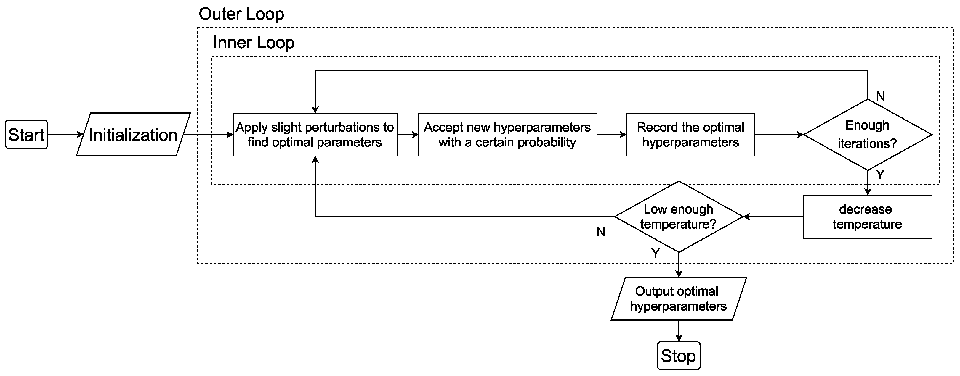
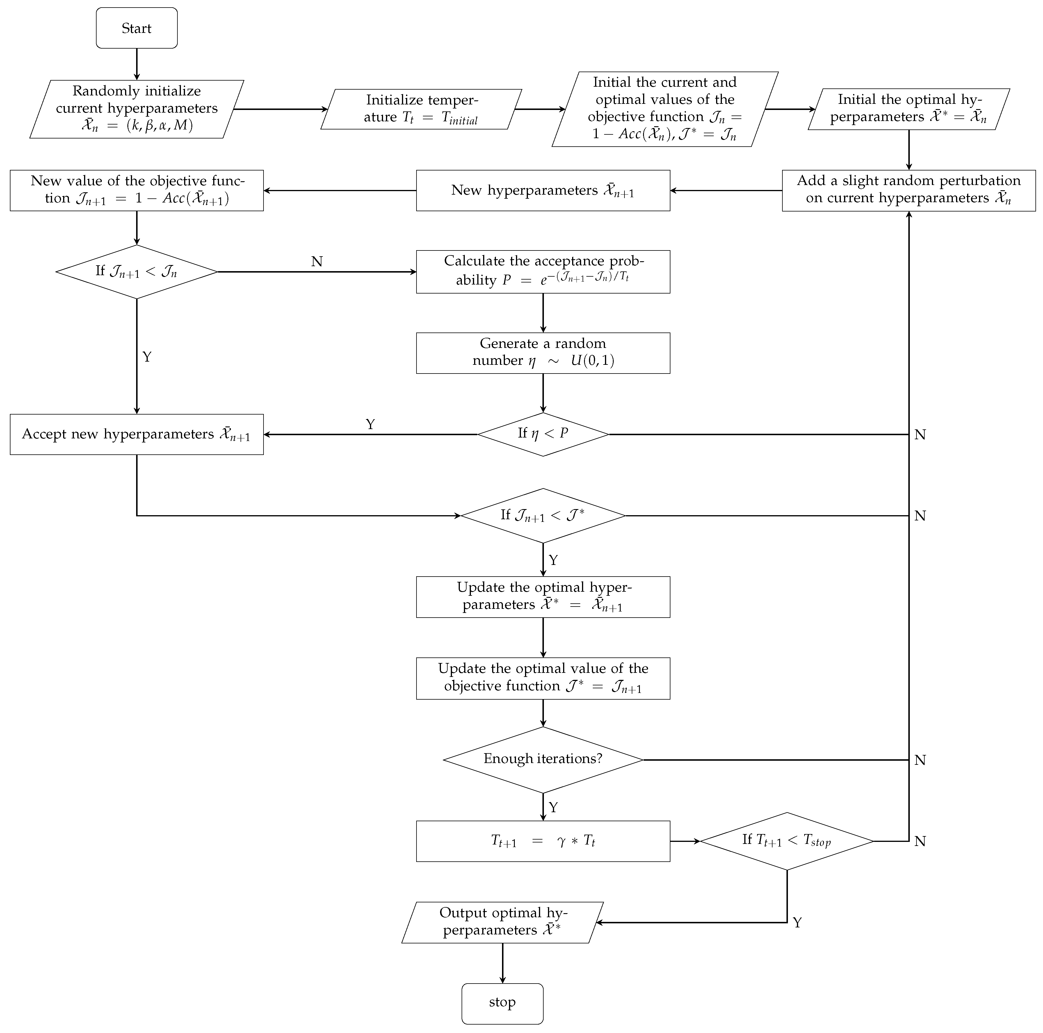
3.4. Self-Adaptive Hyperparameter Optimization Algorithm

3.4.1. Simulated Annealing Algorithm

The simulated annealing algorithm [23] is a probabilistic-based optimization strategy, usually utilized to search the global optimum of an objective function that may have multiple local optima. In the simulated annealing algorithm, the optimization problem is to find a collection of variables $\overline{\mathcal{X}}=\{{\mathcal{X}}_1,{\mathcal{X}}_2,\dots ,{\mathcal{X}}_n\}$, which maximizes or minimizes the value of the objective function $f\left(\overline{\mathcal{X}}\right)$. The hyperparameters of distribution calibration with prototype-based representative mechanism include the power of Tukey’s transformation $\beta$, the number of selected similar classes k, the compensation for the within-class variation $\alpha$, and the number of generated features M. The objective is to seek optimal hyperparameters that lead to the smallest values of mean error rate on 10,000 few-shot classification tasks. The objective function can be given by:

$$\begin{array}{cc}\hfill \mathcal{J}\left(\mathcal{X}\right)& =1-Acc\left(\overline{\mathcal{X}}\right),\hfill \end{array}$$

(16)

where $Acc(·)$ is the operator to calculate mean accuracy on 10,000 classification tasks. The simulated annealing algorithm is a process that simulates a solid being heated and then slowly cooled. In the natural sciences, the temperature has physical significance. However, for the optimization problem, the temperature is only a control parameter. The initial temperature and the stop temperature control the iteration number of the algorithm, represented by $T_{initial}$ and $T_{stop}$. The cooling schedule is given by:

$$\begin{array}{cc}\hfill T_{t+1}& =\gamma \ast T_t,\hfill \end{array}$$

(17)

where $\gamma$ is a constant less than one as the cooling coefficient, $T_t$ is the current temperature in the outer loop, and $T_{t+1}$ is the next temperature in the outer loop.

3.4.2. Metropolis Algorithm

The simulated annealing process aims to find parameters that maximize or minimize the objective function. The hyperparameters change into the neighborhood of the current position with some tiny random perturbation. Correspondingly, the difference in the objective function value caused by this perturbation is denoted as $\Delta \mathcal{J}={\mathcal{J}}_{n+1}-{\mathcal{J}}_n$, where ${\mathcal{J}}_{n+1}$ is the new objective function value resulting from new hyperparameters after perturbation, and ${\mathcal{J}}_n$ is the current value resulting from current hyperparameters before perturbation. When the objective function value decreases ($\Delta \mathcal{J}<0$), new hyperparameters are accepted as the starting point for the next perturbation. When the objective function value increases ($\Delta \mathcal{J}>0$), new hyperparameters may still be accepted with a certain probability, helping escape from the local optimum. The Metropolis algorithm [30] was introduced to generate the probability that determines whether to accept the new parameters. The acceptance probability is given by:

$$\begin{array}{c}\hfill P=e^{-\Delta \mathcal{J}/T_t},\end{array}$$

(18)

where $\Delta \mathcal{J}$ is the difference in the objective function value, and $T_t$ is the current temperature in the outer loop. They control the acceptance probability together. When $\Delta \mathcal{J}$ is the same, the probability is larger at higher temperatures and smaller at lower temperatures. This probabilistic acceptance can be achieved by comparing P with a random number $\eta$ sampled from a continuous uniform distribution $U(0,1)$. When $\eta <P$, the new parameters are accepted.

4. Experiments

4.1. Datasets

The experiments are conducted on three few-shot learning benchmarks, including miniImageNet [6], CUB-200-2011 [31], and CIFAR-FS [32]. miniImageNet is a mini-version of the ImageNet dataset [33], which contains 100 classes with 600 images per class, and the image size is 84 × 84 × 3. miniImageNet is divided into 64 base classes, 16 validation classes, and 20 novel classes in all experiments. CUB-200-2011 is a fine-grained classification dataset that includes bird images of size 84 × 84 × 3, split into 100 base, 50 validation, and 50 novel classes. CIFAR-FS is created by randomly splitting 100 classes of CIFAR-100 [34] into 64 base classes, 16 validation classes, and 20 novel classes. The images are of size 32 × 32 × 3.

4.2. Evaluation Criteria

Experiments are performed on 10,000 tasks randomly sampled from novel classes, following 5-way-1-shot and 5-way-5-shot settings. The task-specific classifiers are evaluated on 15 query images per class in each task. The evaluation metric is the average top-1 accuracy on 10,000 tasks.

4.3. Implementation Details

Following the previous work [17], a WideResNet model is trained on base classes as the feature extractor for each dataset. As the task-specific classifier, we use the logistic regression classifier with L2 regularization. After classifier training, we use it for testing novel classes. The configuration used for all experiments consists of an Nvidia Quadro RTX 5000 (16 GB), 64 GB of RAM, Ubuntu 20.04, and torch 1.7.1.

4.4. Comparison to State-of-the-Art

We compared the proposed framework with other state-of-the-art methods, including optimization-based, metric-based, fine-tuning-based, and generation-based.

Table 1. 5-way-1-shot and 5-way-5-shot classification accuracy (%) on miniImageNet with 95% confidence intervals.

Method		miniImageNet
		5-way-1-shot	5-way-5-shot
Optimization-based	ICML17’ MAML [4]	$48.70\pm 1.75$	$63.11\pm 0.92$
	Meta-SGD [35]	$50.47\pm 1.87$	$64.03\pm 0.94$
	ICML18’ adaResNet [36]	$56.88\pm 0.62$	$71.94\pm 0.57$
	ICLR19’ LEO [37]	$61.76\pm 0.08$	$77.59\pm 0.12$
	ECCV20’ E3BM [38]	$63.8\pm 0.4$	$80.29\pm 0.25$
	CVPR19’ Meta Transfer Learning [39]	$64.3\pm 1.7$	$80.9\pm 0.8$
Metric-based	NIPS16’ MatchingNet [6]	$43.44\pm 0.77$	$55.31\pm 0.73$
	NIPS17’ ProtoNet [14]	$49.42\pm 0.78$	$68.20\pm 0.66$
	CVPR18’ RelationNet [40]	$50.44\pm 0.82$	$65.32\pm 0.70$
	NIPS19’ CAN [41]	$63.85\pm 0.48$	$79.44\pm 0.34$
	AAAI22’ AAP2S [42]	$64.82\pm 0.12$	$81.31\pm 0.22$
Fine-tuning-based	ICLR19’ Baseline++ [15]	$53.97\pm 0.79$	$75.90\pm 0.61$
	ECCV20’ RFS-simple [16]	$62.02\pm 0.63$	$79.64\pm 0.44$
	WACV20’ S2M2${}_R$ [17]	$64.93\pm 0.18$	$83.18\pm 0.11$
	ECCV20’ Negative-Cosine [43]	$62.33\pm 0.82$	$80.94\pm 0.59$
Generation-based	TPAMI21’ DC [10]	$68.15\pm 0.20$	$83.52\pm 0.14$
	NIPS18’ MetaGAN [18]	$52.71\pm 0.64$	$68.63\pm 0.67$
	NIPS18’ Delta-Encoder [19]	$59.9$	$69.7$
	TIP19’ TriNet [44]	$58.12\pm 1.37$	$76.92\pm 0.69$
	ICML20’ Meta Variance Transfer [45]	-	$67.67\pm 0.70$
Ours	PSDC	$\mathbf{68.31}\pm \mathbf{0.20}$	$\mathbf{83.75}\pm \mathbf{0.13}$

and

Table 2. 5-way-1-shot and 5-way-5-shot classification accuracy (%) on CUB-200-2011 with 95% confidence intervals.

Method		CUB-200-2011
		5-way-1-shot	5-way-5-shot
Optimization-based	ICML17’ MAML [4]	$50.45\pm 0.97$	$59.60\pm 0.84$
	Meta-SGD [35]	$53.34\pm 0.97$	$67.59\pm 0.82$
Metric-based	NIPS16’ MatchingNet [6]	$73.49\pm 0.89$	$84.45\pm 0.58$
	NIPS17’ ProtoNet [14]	$72.99\pm 0.88$	$86.64\pm 0.51$
	CVPR18’ RelationNet [40]	$68.65\pm 0.91$	$81.12\pm 0.63$
	AAAI22’ AAP2S [42]	$77.64\pm 0.19$	$90.43\pm 0.18$
Fine-tuning-based	ICLR19’ Baseline++ [15]	$69.55\pm 0.89$	$85.17\pm 0.50$
	ECCV20’ Negative-Cosine [43]	$72.66\pm 0.85$	$89.40\pm 0.43$
Generation-based	TPAMI21’ DC [10]	$80.29\pm 0.20$	$90.80\pm 0.11$
	NIPS18’ Delta-Encoder [19]	$69.8$	$82.6$
	TIP19’ TriNet [44]	$69.61\pm 0.46$	$84.10\pm 0.35$
	ICML20’ Meta Variance Transfer [45]	-	$80.33\pm 0.6$
Ours	PSDC	$\mathbf{80.43}\pm \mathbf{0.20}$	$\mathbf{91.16}\pm \mathbf{0.10}$

present the classification results of our framework for 5-way-1-shot and 5-way-5-shot on miniImageNet and CUB-200-2011, respectively.

Table 3. 5-way-1-shot and5-way-5-shot classification accuracy (%) on CIFAR-FS with 95% confidence intervals.

Method		CIFAR-FS
		5-way-1-shot	5-way-5-shot
Optimization-based	ICML17’ MAML [4]	$58.9\pm 1.9$	$71.5\pm 1.0$
	ICLR19’ R2D2 [32]	$65.4\pm 0.2$	$79.4\pm 0.2$
	CVPR19’ MetaOptNet [46]	$72.8\pm 0.7$	$85.0\pm 0.5$
Metric-based	NIPS17’ ProtoNet [14]	$55.5\pm 0.7$	$72.0\pm 0.6$
	CVPR18’ RelationNet [40]	$55.0\pm 1.0$	$69.3\pm 0.8$
	AAAI22’ AAP2S [42]	$73.12\pm 0.22$	$85.69\pm 0.16$
	CVPR19’ Shot-Free [47]	$69.15$	$84.70$
Fine-tuning-based	ICLR19’ Baseline++ [15]	$67.50\pm 0.64$	$80.08\pm 0.32$
Ours	PSDC	$\mathbf{74.66}\pm \mathbf{0.21}$	$\mathbf{86.37}\pm \mathbf{0.15}$

displays the results on CIFAR-FS. All tables show that our framework achieves the best performance for 1-shot and 5-shot compared with the other state-of-the-art on miniImageNet, CUB-200-2011, and CIFAR-FS.

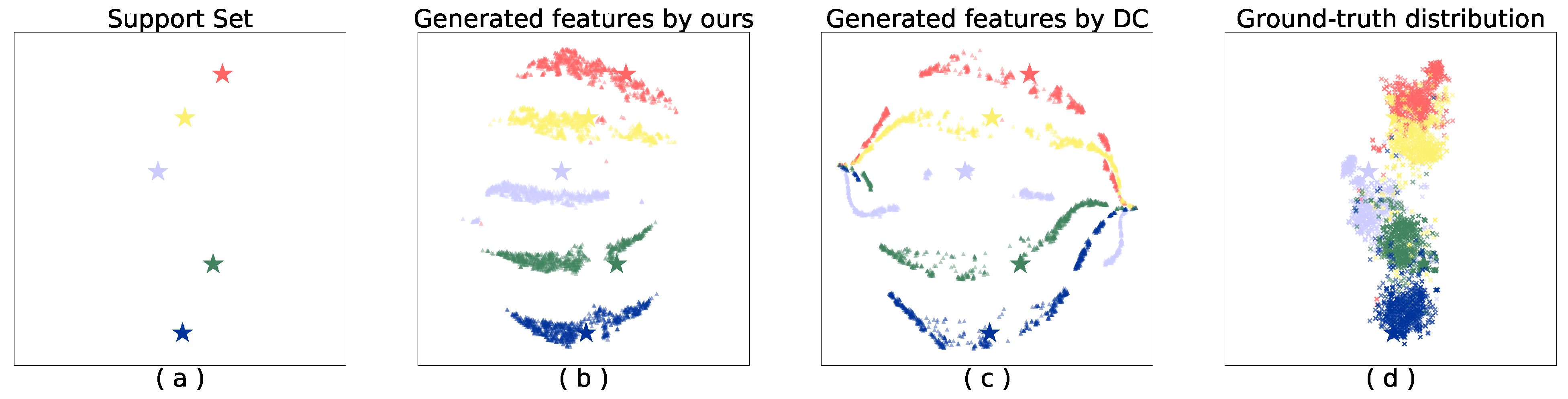
4.5. Visualization of Generated Samples

A task for 5-way-1-shot is randomly sampled from novel classes of miniImageNet. Figure 4 shows the t-SNE [48] visualization of the ground-truth distributions and the generated features on the task. Figure 4a presents the support set in the task, which includes five samples. We show the features generated by PSDC in Figure 4b, the features generated by DC [10] in Figure 4c, and the ground-truth feature distributions in Figure 4d. From Figure 4, we can observe that the feature distributions generated by PSDC are more aggregated and consistent with the corresponding ground-truth distributions than those generated by DC. The visualization illustrates the inherent plausibility of our method in the accuracy improvement of the few-shot classification task.

4.6. Ablation Study

The results of the ablation study are reported in

Table 4. Ablation study on miniImageNet and CUB-200-2011 for 5-way-1-shot and 5-way-5-shot settings, the experiment.

PRM	SHOA	miniImageNet		CUB-200-2011
		5-way-1-shot	5-way-5-shot	5-way-1-shot	5-way-5-shot
×	×	$68.15\pm 0.20$	$83.52\pm 0.14$	$80.29\pm 0.20$	$90.80\pm 0.11$
✓	×	-	$83.65\pm 0.14$	-	$90.88\pm 0.11$
×	✓	$\mathbf{68.31}\pm \mathbf{0.20}$	$83.65\pm 0.14$	$\mathbf{80.43}\pm \mathbf{0.20}$	$91.09\pm 0.10$
✓	✓	-	$\mathbf{83.75}\pm \mathbf{0.13}$	-	$\mathbf{91.16}\pm \mathbf{0.10}$

to show the different effects of multiple ingredients in the proposed framework, including the effects of Prototype-based Representative Mechanism (PRM) and the Self-adaptive Hyperparameter Optimization Algorithm (SHOA). Experiments of the ablation study are conducted on 10,000 tasks, and the reported results are the average classification accuracy with a 95% confidence interval. The baseline is the classification performance of the model when no components of the Prototype-based Adaptive Distribution Calibration (PSDC) framework are used.

4.6.1. Ablation Study on the Prototype-Based Representative Mechanism

In the case of the 5-way-1-shot, there are five classes in the support set, and each class has a single sample that is the prototype-based representative. Therefore, the Prototype-based Representative Mechanism is applied for 5-shot, and we use “-” to replace the same result in Table 4. In the case of the 5-way-5-shot, when the model is trained without SHOA, PRM can improve the performance by 0.13% on miniImageNet, and the performance gain is 0.08% on CUB-200-2011. When the model is trained with SHOA, PRM can improve the performance by 0.1% and 0.07% on the miniImageNet and CUB-200-2011, respectively.

4.6.2. Ablation Study on the Self-Adaptive Hyperparameter Optimization Algorithm

Table 4 shows that, when the model is trained without PRM, SHOA can improve the performance by 0.16% and 0.13% on miniImageNet for 1-shot and 5-shot, respectively. Moreover, the model performance has been improved by 0.14% and 0.29% on the CUB-200-2011 for 1-shot and 5-shot, respectively. When the model is trained with PRM, SHOA can improve the performance by 0.1% and 0.28% for 5-shot on miniImageNet and CUB-200-2011, respectively. The results of ablation experiments illustrate that SHOA can not only self-adaptively optimize hyperparameters for the distribution calibration of different application scenarios (i.e., datasets) but also build a robust distribution calibration model for few-shot image classification.

4.6.3. Ablation Study on PRM and SHOA

Table 4 shows that, when the model is trained with PRM and SHOA, model performance compared with baseline can be improved by 0.23% and 0.36% for 5-shot on miniImageNet and CUB-200-2011, respectively. The results of the ablation experiment illustrate that the classification performance of models can be improved by using both PRM and SHOA in the few-shot image classification task.

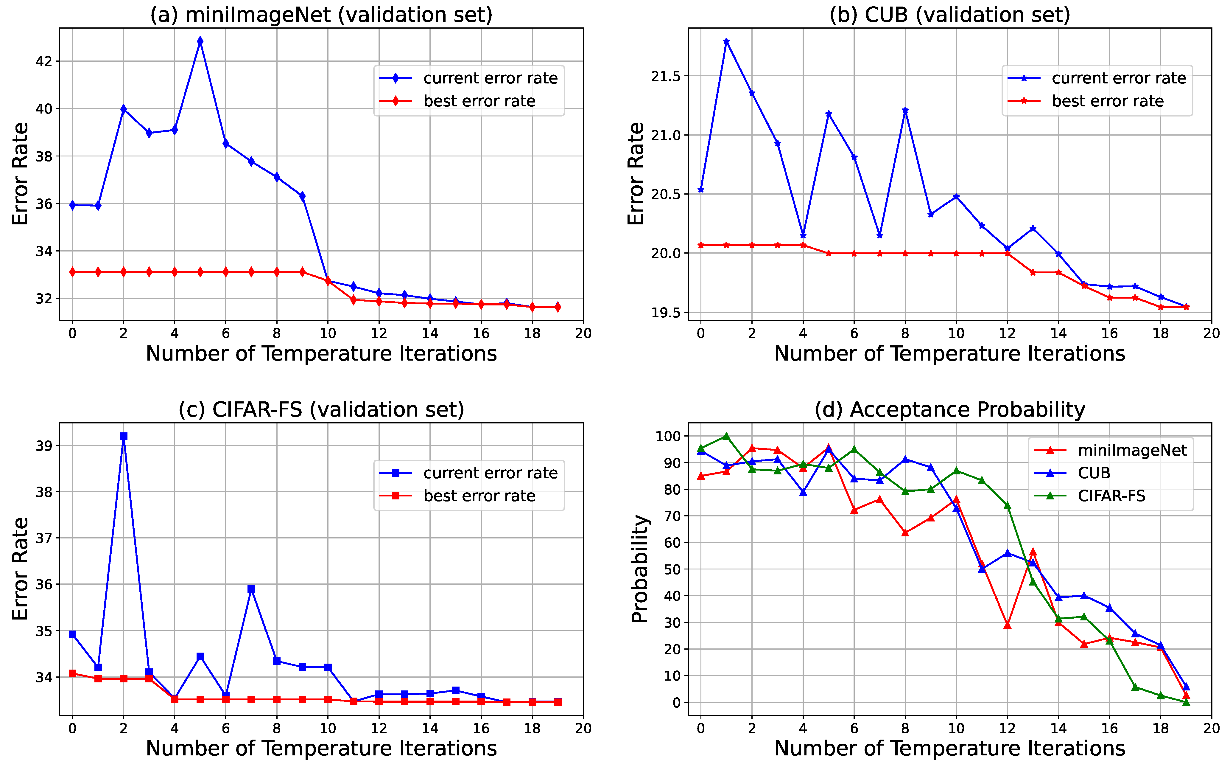
4.7. Hyperparameter Searching

The hyperparameters are searched on the validation set. The optimal hyperparameters achieve the lowest error rate, i.e., the highest accuracy. Before hyperparameter searching, some parameters need to be initialized, including the current and optimal hyperparameters of distribution calibration, the temperature for controlling acceptance probability, and the current and optimal values of the objective function (i.e., accuracy or error rate).

In the inner loop, a slight perturbation is added to a random hyperparameter, resulting in a new error rate. We compare the new error rate with the current error rate. In the first case, the new hyperparameters are accepted if the new error rate is less than the current error rate. In the other case, if the new error rate is greater than or equal to the current error rate, the acceptance probability is determined by the current temperature and the difference between the new error rate and the current error rate as Equation (18), which helps jump out of the local minimum. Suppose new hyperparameters are accepted, and the new error rate is lower than the optimal error rate. In that case, the optimal error rate and the optimal hyperparameters are updated by the new error rate and new hyperparameter.

As the number of outer loops increases, the temperature decay is performed according to Equation (17). The acceptance probability decreases considerably to almost zero as the temperature decays. The whole hyperparameter optimization is repeated continuously by a certain number of iterations, and robust hyperparameters can be found that are approximately the global optimum. Our method can make the objective function converge to the globally optimal value by jumping out of the locally optimal value with a certain probability. Furthermore, it can automatically search for the appropriate values of the hyperparameters rather than manually setting them, implementing the self-adaptive hyperparameter optimization for different application scenarios (i.e., datasets).

We present the process of hyperparameter optimization in Figure 5. Figure 5a–c show the variation of the model error rate on three different validation sets as the temperature iterations increase. The red line displays the evolution of the best model performance. The blue line represents the model performance at the last iteration of the inner loop. In addition, we show the variable acceptance probability at the last iteration of the inner loop as the number of temperature iterations increases in Figure 5d. Figure 5 shows that, as the number of temperature iterations increases, the model classification performance gradually coincides with the optimal classification performance, and the acceptance probability gradually decreases.

5. Conclusions

This paper proposes a novel few-shot image classification framework—Prototype-based Self-adaptive Distribution Calibration (PSDC), which includes a prototype-based representative mechanism and a self-adaptive hyperparameter optimization algorithm. To the best of our knowledge, PSDC is the first attempt to utilize a self-adaptive strategy in the hyperparameter optimization of distribution calibration. Extensive experiments are conducted on the miniImageNet, CUB-200-2011, and CIFAR-FS. Experimental results indicate that PSDC surpasses other few-shot learning methods on three benchmarks. Furthermore, the visualization of the generated features verifies that PSDC can better estimate the ground-truth distribution. All results verify the effectiveness of the proposed framework and demonstrate that PSDC achieves state-of-the-art. However, since the current algorithm for estimating the ground-truth distribution is still hand-crafted, future work will focus on learning distribution by deep neural networks to estimate the ground-truth distributions accurately.

References

1. Ye, H.; Hu, H.; Zhan, D. Learning Adaptive Classifiers Synthesis for Generalized Few-Shot Learning. Int. J. Comput. Vis. 2021, 129, 1930–1953. [Google Scholar] [CrossRef]
2. Xu, W.; Xian, Y.; Wang, J.; Schiele, B.; Akata, Z. Attribute Prototype Network for Any-Shot Learning. Int. J. Comput. Vis. 2022, 130, 1735–1753. [Google Scholar] [CrossRef]
3. Koniusz, P.; Zhang, H. Power Normalizations in Fine-Grained Image, Few-Shot Image and Graph Classification. IEEE Trans. Pattern Anal. Mach. Intell. 2022, 44, 591–609. [Google Scholar] [CrossRef] [PubMed]
4. Finn, C.; Abbeel, P.; Levine, S. Model-Agnostic Meta-Learning for Fast Adaptation of Deep Networks. In Proceedings of the 34th International Conference on Machine Learning, Sydney, Australia, 6–11 August 2017; pp. 1126–1135. [Google Scholar]
5. Raghu, A.; Raghu, M.; Bengio, S.; Oriol, V. Rapid Learning or Feature Reuse? Towards Understanding the Effectiveness of MAML. In Proceedings of the 8th International Conference on Learning Representations, Online, 26–30 April 2020. [Google Scholar]
6. Vinyals, O.; Blundell, C.; Lillicrap, T.; Kavukcuoglu, K.; Wierstra, D. Matching Networks for One Shot Learning. In Proceedings of the 30th International Conference on Neural Information Processing Systems (NIPS’16), Barcelona, Spain, 5–10 December 2016; pp. 3637–3645. [Google Scholar]
7. Kang, D.; Kwon, H.; Min, J.; Cho, M. Relational Embedding for Few-Shot Classification. In Proceedings of the IEEE International Conference on Computer Vision, Online, 11–17 October 2021; pp. 8822–8833. [Google Scholar]
8. Bendre, N.; Desai, K.; Najafirad, P. Generalized Zero-Shot Learning Using Multimodal Variational Auto-Encoder With Semantic Concepts. In Proceedings of the 28th IEEE International Conference on Image Processing (ICIP), Online, 19–22 September 2021; pp. 1284–1288. [Google Scholar]
9. Li, K.; Zhang, Y.; Li, K.; Fu, Y. Adversarial Feature Hallucination Networks for Few-Shot Learning. In Proceedings of the IEEE Conference on Computer Vision and Pattern Recognition, Online, 14–19 June 2020; pp. 13470–13479. [Google Scholar]
10. Yang, S.; Wu, S.; Liu, T.; Xu, M. Bridging the Gap between Few-Shot and Many-Shot Learning via Distribution Calibration. IEEE Trans. Pattern Anal. Mach. Intell. 2022, 44, 9830–9843. [Google Scholar] [CrossRef] [PubMed]
11. Bergstra, J.; Bengio, Y. Random search for hyper-parameter optimization. J. Mach. Learn. Res. 2012, 13, 281–305. [Google Scholar]
12. Joy, T.T.; Rana, S.; Gupta, S.; Venkatesh, S. Hyperparameter tuning for big data using Bayesian optimisation. In Proceedings of the 23rd International Conference on Pattern Recognition (ICPR), Cancun, Mexico, 4–8 December 2016; pp. 2574–2579. [Google Scholar]
13. Yu, T.; Zhu, H. Hyper-parameter optimization: A review of algorithms and applications. arXiv 2020, arXiv:2003.05689. [Google Scholar]
14. Snell, J.; Swersky, K.; Zemel, R. Prototypical Networks for Few-shot Learning. In Proceedings of the 31st International Conference on Neural Information Processing Systems (NIPS’17), Long Beach, CA, USA, 4–9 December 2017; pp. 4080–4090. [Google Scholar]
15. Chen, W.-Y.; Liu, Y.-C.; Kira, Z.; Wang, Y.-C.F.; Huang, J.-B. A Closer Look at Few-shot Classification. In Proceedings of the 7th International Conference on Learning Representations, New Orleans, LA, USA, 6–9 May 2019. [Google Scholar]
16. Tian, Y.; Wang, Y.; Krishnan, D.; Tenenbaum, J.B.; Isola, P. Rethinking Few-Shot Image Classification: A Good Embedding is All You Need? In Computer Vision–ECCV 2020 (Lecture Notes in Computer Science); Springer: Cham, Switzerland, 2020; pp. 266–282. [Google Scholar]
17. Mangla, P.; Kumari, N.; Sinha, A.; Singh, M.; Krishnamurthy, B.; Balasubramanian, V.N. Charting the Right Manifold: Manifold Mixup for Few-shot Learning. In Proceedings of the IEEE/CVF Winter Conference on Applications of Computer Vision (WACV), Snowmass Village, CO, USA, 1–5 March 2020; pp. 2207–2216. [Google Scholar]
18. Zhang, R.; Che, T.; Ghahramani, Z.; Bengio, Y.; Song, Y. MetaGAN: An Adversarial Approach to Few-Shot Learning. In Proceedings of the 32nd Conference on Neural Information Processing Systems (NIPS’18), Montreal, QC, Canada, 3–8 December 2018; pp. 2371–2380. [Google Scholar]
19. Schwartz, E.; Karlinsky, L.; Shtok, J.; Harary, S.; Marder, M.; Kumar, A.; Feris, R.; Giryes, R.; Bronstein, A. Delta-encoder: An effective sample synthesis method for few-shot object recognition. In Proceedings of the 32nd Conference on Neural Information Processing Systems (NIPS’18), Montreal, QC, Canada, 3–8 December 2018; pp. 2850–2860. [Google Scholar]
20. Zhang, J.; Zhao, C.; Ni, B.; Xu, M.; Yang, X. Variational Few-Shot Learning. In Proceedings of the IEEE International Conference on Computer Vision, Long Beach, CA, USA, 16–20 June 2019; pp. 1685–1694. [Google Scholar]
21. Hong, Y.; Niu, L.; Zhang, J.; Zhang, L. Matchinggan: Matching-Based Few-Shot Image Generation. In Proceedings of the IEEE International Conference on Multimedia and Expo, Online, 6–10 July 2020; pp. 1–6. [Google Scholar]
22. Goodfellow, I.; Pouget-Abadie, J.; Mirza, M.; Xu, B.; Warde-Farley, D.; Ozair, S.; Courville, A.; Bengio, Y. Generative Adversarial Nets. Commun. ACM 2020, 63, 139–144. [Google Scholar] [CrossRef]
23. Kirkpatrick, S.; Gelatt Jr, C.D.; Vecchi, M.P. Optimization by simulated annealing. Science 1983, 220, 671–680. [Google Scholar] [CrossRef] [PubMed]
24. Kassaymeh, S.; Al-Laham, M.; Al-Betar, M.A.; Alweshah, M.; Abdullah, S.; Makhadmeh, S.N. Backpropagation Neural Network optimization and software defect estimation modelling using a hybrid Salp Swarm optimizer-based Simulated Annealing Algorithm. Knowl. Based. Syst. 2022, 244, 108511. [Google Scholar] [CrossRef]
25. Bandyopadhyay, R.; Basu, A.; Cuevas, E.; Sarkar, R. Harris Hawks optimisation with Simulated Annealing as a deep feature selection method for screening of COVID-19 CT-scans. Appl. Soft Comput. 2021, 111, 107698. [Google Scholar] [CrossRef] [PubMed]
26. Rere, L.M.R.; Fanany, M.I.; Arymurthy, A.M. Simulated Annealing Algorithm for Deep Learning. Procedia Comput. Sci. 2015, 72, 137–144. [Google Scholar] [CrossRef] [Green Version]
27. Ayumi, V.; Rere, L.M.R.; Fanany, M.I.; Arymurthy, A.M. Optimization of convolutional neural network using microcanonical annealing algorithm. In Proceedings of the 8th International Conference on Advanced Computer Science and Information Systems, Malang, Indonesia, 15–16 October 2016; pp. 506–511. [Google Scholar]
28. Hu, Z.; Zhou, L.; Jin, B.; Liu, H. Applying improved convolutional neural network in image classification. Mob. Netw. Appl. 2020, 25, 133–141. [Google Scholar] [CrossRef]
29. Tukey, J.W. Exploratory Data Analysis; Addison-Wesley: Reading, MA, USA, 1977; pp. 1–704. [Google Scholar]
30. Metropolis, N.; Rosenbluth, A.W.; Rosenbluth, M.N.; Teller, A.H.; Teller, E. Equation of state calculations by fast computing machines. J. Chem. Phys. 1953, 21, 1087–1092. [Google Scholar] [CrossRef] [Green Version]
31. Welinder, P.; Branson, S.; Mita, T.; Wah, C.; Schroff, F.; Belongie, S.; Perona, P. The Caltech-ucsd Birds-200; CNS-TR-2010-001; California Institute of Technology: Pasadena, CA, USA, 2010. [Google Scholar]
32. Bertinetto, L.; Henriques, J.F.; Torr, P.; Vedaldi, A. Meta-learning with differentiable closed-form solvers. In Proceedings of the 7th International Conference on Learning Representations, New Orleans, LA, USA, 6–9 May 2019. [Google Scholar]
33. Russakovsky, O.; Deng, J.; Su, H.; Krause, J.; Satheesh, S.; Ma, S.; Huang, Z.; Karpathy, A.; Khosla, A.; Bernstein, M.; et al. ImageNet Large Scale Visual Recognition Challenge. Int. J. Comput. Vis. 2015, 115, 211–252. [Google Scholar] [CrossRef] [Green Version]
34. Krizhevsky, A.; Hinton, G. Learning Multiple Layers of Features from Tiny Images; University of Toronto: Toronto, ON, Canada, 2009. [Google Scholar]
35. Li, Z.; Zhou, F.; Chen, F.; Li, H. Meta-SGD: Learning to Learn Quickly for Few-Shot Learning. arXiv 2017, arXiv:1707.09835. [Google Scholar]
36. Munkhdalai, T.; Yuan, X.; Mehri, S.; Trischler, A. Rapid Adaptation with Conditionally Shifted Neurons. In Proceedings of the 35th International Conference on Machine Learning, Stockholm, Sweden, 10–15 July 2018; pp. 3664–3673. [Google Scholar]
37. Rusu, A.A.; Rao, D.; Sygnowski, J.; Vinyals, O.; Pascanu, R.; Osindero, S.; Hadsell, R. Meta-Learning with Latent Embedding Optimization. In Proceedings of the 7th International Conference on Learning Representations, New Orleans, LA, USA, 6–9 May 2019. [Google Scholar]
38. Liu, Y.; Schiele, B.; Sun, Q. An Ensemble of Epoch-Wise Empirical Bayes for Few-Shot Learning. In Computer Vision–ECCV 2020 (Lecture Notes in Computer Science); Springer: Cham, Switzerland, 2020; pp. 404–421. [Google Scholar]
39. Sun, Q.; Liu, Y.; Chua, T.; Schiele, B. Meta-Transfer Learning for Few-Shot Learning. In Proceedings of the IEEE Conference on Computer Vision and Pattern Recognition, Long Beach, CA, USA, 16–20 June 2019; pp. 403–412. [Google Scholar]
40. Sung, F.; Yang, Y.; Zhang, L.; Xiang, T.; Torr, P.H.S.; Hospedales, T.M. Learning to Compare: Relation Network for Few-Shot Learning. In Proceedings of the IEEE Conference on Computer Vision and Pattern Recognition, Salt Lake City, UT, USA, 18–22 June 2018; pp. 1199–1208. [Google Scholar]
41. Hou, R.; Chang, H.; Ma, B.; Shan, S.; Chen, X. Cross Attention Network for Few-shot Classification. In Proceedings of the 33th International Conference on Neural Information Processing Systems (NIPS’19), Vancouver, BC, Canada, 8–14 December 2019; pp. 4003–4014. [Google Scholar]
42. Ma, R.; Fang, P.; Drummond, T.; Harandi, M. Adaptive Poincaré Point to Set Distance for Few-Shot Classification. In Proceedings of the 36th AAAI Conference on Artificial Intelligence, Online, 22 February–1 March 2022; pp. 1926–1934. [Google Scholar]
43. Liu, B.; Cao, Y.; Lin, Y.; Li, Q.; Zhang, Z.; Long, M.; Hu, H. Negative Margin Matters: Understanding Margin in Few-Shot Classification. In Computer Vision–ECCV 2020 (Lecture Notes in Computer Science); Springer: Cham, Switzerland, 2020; pp. 438–455. [Google Scholar]
44. Chen, Z.; Fu, Y.; Zhang, Y.; Jiang, Y.; Xue, X.; Sigal, L. Multi-Level Semantic Feature Augmentation for One-Shot Learning. IEEE Trans. Image Process. 2019, 28, 4594–4605. [Google Scholar] [CrossRef] [PubMed]
45. Park, S.; Han, S.; Baek, J.; Kim, I.; Song, J.; Lee, H.B.; Han, J.; Hwang, S.J. Meta Variance Transfer: Learning to Augment from the Others. In Proceedings of the 37th International Conference on Machine Learning, Online, 13–18 July 2020; pp. 7510–7520. [Google Scholar]
46. Lee, K.; Maji, S.; Ravichandran, A.; Soatto, S. Meta-Learning With Differentiable Convex Optimization. In Proceedings of the IEEE Conference on Computer Vision and Pattern Recognition, Long Beach, CA, USA, 16–20 June 2019; pp. 10649–10657. [Google Scholar]
47. Ravichandran, A.; Bhotika, R.; Soatto, S. Few-Shot Learning With Embedded Class Models and Shot-Free Meta Training. In Proceedings of the IEEE International Conference on Computer Vision, Seoul, Republic of Korea, 26 October–2 November 2019; pp. 331–339. [Google Scholar]
48. Van der Maaten, L.; Hinton, G. Visualizing Data using t-SNE. J. Mach. Learn. Res. 2008, 9, 2579–2605. [Google Scholar]
Figure 1. The pipeline of distribution calibration with the Prototype-based Representative Mechanism.
Electronics 12 00134 g001
Figure 2. The basic block diagram of the Self-Adaptive Hyperparameter Optimization Algorithm, which contains two loops. In the inner loop, a slight perturbation is applied to the current hyperparameters, which are accepted with a certain probability. In the outer loop, the temperature decreases from a high value to a pre-set stop temperature.
Electronics 12 00134 g002
Figure 3. The flow diagram of the Self-Adaptive Hyperparameter Optimization Algorithm. As the temperature decreases, the acceptance probability decreases, helping jump out of the local minimum.
Electronics 12 00134 g003
Figure 4. The t-SNE visualization of generated features and ground-truth distributions on a random 5-way-1-shot task sampled from miniImageNet. ★ in (ad) represents support set features, ▲ in (b,c) represents the generated features, × in figure (d) represents features of ground-truth distributions.
Electronics 12 00134 g004
Figure 5. Visualization of the error rate and acceptance probability on validation sets of miniImageNet, CUB-200-2011, and CIFAR-FS. (a) The variation of the model error rate on the validation set of miniImageNet as the temperature iterations increase. (b) The variation of the model error rate on the validation set of CUB-200-2011 as the temperature iterations increase. (c) The variation of the model error rate on the validation set of CIFAR-FS as the temperature iterations increase. (d) The variation of acceptance probability on three datasets as the number of temperature iterations increases.
Electronics 12 00134 g005