Simulation-Based Testing of Subsystems for Autonomous Vehicles at the Example of an Active Suspension Control System

Abstract

Automated driving functions are expected to increase both the safety and ride comfort of future vehicles. Ensuring their functional safety and optimizing their performance requires thorough testing. Costs and duration of tests can be reduced if more tests can be performed numerically in a feasible simulation framework. This simulation setup must include all subsystems of the autonomous vehicle, which significantly interact with the system under test. In this paper, a modular model chain is presented, which is developed for testing systems with an impact on vehicle motion. It includes trajectory planning, motion control, and a model of the vehicle dynamics in a closed loop. Each subsystem can easily be exchanged to adapt the model chain with respect to the simulation objectives. As a use case, the testing of an active suspension control system is discussed. It is designed directly for use in autonomous cars and uses inputs from the vehicle motion planning subsystem for planning the suspension actuator motion. Using the presented closed-loop model chain, the effect of different actuator control strategies on ride comfort is compared, such as curve tilting. Furthermore, the impact of the active suspension system on lateral vehicle motion is shown.

1. Introduction

Automated driving is currently one of the major research topics in the automotive field, mainly motivated by the improvement of driving safety [1]. The improvement of driving safety is supposed to be obtained by replacing the human driver with a complex system including sensors for detecting the environment, a so-called highly automated driving (HAD) function, and actuators. Testing and validation of automated vehicles including the mutual interaction of auxiliary systems that influence driving dynamics are fundamental steps in the development process to ensure the required safety performance and therefore play a key role in the future success of automated driving [2].

One of the major challenges of testing and validating automated vehicles is covering the enormous amount of possible driving situations, due to the complexity and the high number of variables of the interaction of a vehicle with the environment and other traffic agents including rare events [3]. Therefore, replacing a high quote of real driving tests with simulation leads to a major benefit for the development of automated vehicles. For complex mechatronic systems, shifting tests to simulation means also shortening the development process and improving its flexibility. Some examples of simulation frameworks with a focus on scenario-based testing of the behavior of the vehicle can be found in [4,5,6]. Others are developed with a focus on fault injection and failure analysis [7,8] The SET Level project, supported by the German Federal Ministry of Economic Affairs and Climate Action, aims at providing an environment for simulation-based tests and the development of automated driving functions, which is flexible to be used for a large variety of different test objectives [9].

HAD also leads to a change of the conceptual focus from the vehicle as a means of transport to a space with the ability to work, communicate or sleep. In [10], the quality of secondary activity is identified as one of four additional customer-relevant properties in automated vehicles. To enable undisturbed secondary activities, the exposition of the occupants to accelerations due to driving dynamics should be minimized [11]. Since the chassis represents the connection between road and occupants, it still plays an important role in passenger comfort also in autonomous driving cars.

To improve ride comfort and enable secondary activities, active suspension systems, such as the “predictive active suspension” from Audi AG [12] and the “e-active body control” from Mercedes Benz AG [13] became popular over the last years. Such systems offer the ability to apply forces to each corner of the car independently from road excitation. Therefore, it is possible to adjust the forces acting on the occupants by, e.g., active curve tilting, where the vehicle is tilted to the inner side of the curve, or a helicopter mode, where braking and accelerating get partly compensated by a counteracting active pitch motion. The active suspension also helps to meet the increasing comfort requirements of automated vehicles [13]. Automated vehicles offer additional information, such as the planned future trajectory of the vehicle, which can be used as preview information for the active suspension control algorithm [14].

In the following sections, a toolchain and a procedure are presented to show the capabilities of virtual development and validation for a vertical trajectory control to improve ride comfort and safety in an automated vehicle. Section 2 describes the framework and models for simulation-based testing of subsystems. The application of the framework is executed on the example of an active suspension control system in Section 3 with a description of a concrete system under test, a test scenario, and simulation results. An overall assessment of simulation-based testing of subsystems for autonomous vehicles is given in the conclusion in Section 4.

2. Model Chain for Subsystem Tests

An automated driving function is a complex system consisting of several subsystems [15], including hardware, like sensors and actuators as well as software modules for data interpretation and action planning. Typical autonomous driving functions use environment sensors, like LIDAR, RADAR, and cameras to observe the environment. The data generated by these sensors are analyzed by software algorithms, which identify objects, like obstacles, and interpret the scenery including the intention and expected future motion of other traffic participants. Based on this scene interpretation, a decision-making layer decides on the future behavior of the ego-vehicle, e.g., which lane to choose or whether the ego-vehicle shall follow or overtake a preceding vehicle. Subsequently, the trajectory for the maneuver is planned and controlled by the vehicle motion controller.

For simulation-based testing of vehicle subsystems, first, the system under test (SUT) and the test objective need to be defined. Then, the subsystems to be included in a closed-loop simulation must be selected. These are typically all subsystems, which have relevant bidirectional interaction with the SUT. The required level of detail for the subsystem models depends on the intensity of interaction with the SUT. If the purpose of the SUT is to influence the vehicle dynamics (e.g., motion control or vehicle actuators), it is typically not necessary to include a camera model and a decision-making algorithm in a closed-loop simulation, even though vehicle dynamics might slightly influence the sensor data by its impact on the field of view. However, if the sensor and scene interpretation subsystems are still able to fully interpret the current traffic scene (which is a requirement for any automated driving system), this would not influence the planned vehicle motion.

Figure 1 shows a closed-loop simulation architecture, which is intended for tests of subsystems with a strong relation to vehicle dynamics, like motion control and vehicle actuators. This architecture is also used for testing the active suspension system in Section 3.

It includes a model of the vehicle dynamics and the closed-loop control of its lateral and longitudinal motion as well as the trajectory planning, which may also react interactively to the actual vehicle motion. Sensors, scene interpretation, and decision-making are not included in the loop. Their inputs to the trajectory planner define the test scenario. These inputs may change during the simulation time according to the test description, but without dependence on the simulation results. The inputs of the trajectory planner are the following:

• reference curve: centerline of the lane to follow according to the decision-making algorithm;
• obstacle trajectories: expected future trajectory of other traffic participants;
• vehicle dynamic limits: limits of the vehicle originating from engine, tire, or steering, which have to be considered for the feasibility of the trajectories and might change in case of a malfunction in a vehicle subsystem (see Equations (5)–(9) in Section 2.1);
• planning parameters: parameters, like weighting factors, search space boundaries, and discretization parameters, which might be changed by a decision-making algorithm depending on the current driving situation (see Section 2.1).

Some of the features like considering obstacles and malfunctions are not needed for the application presented in this paper and will not be discussed in detail in the following. Nevertheless, they are implemented to make the model chain flexible to be also used for other use cases.

The output of the trajectory planner is a trajectory including position, longitudinal velocity, acceleration, heading angle, and curvature for a given time interval. The motion controller compares this trajectory with the corresponding values of the actual vehicle dynamic state and computes a desired vehicle action in terms of a desired longitudinal acceleration and the desired curvature. These values need to be interpreted by the actuator management of the vehicle actuators in terms of, e.g., steering angle or steering force and engine torque. These quantities are not computed directly by the motion controller, to make the motion controller independent from the architecture of the vehicle actuation system. This allows the easier exchange of subsystem models of the vehicle or even the vehicle model itself. A more detailed description of the subsystems included in the simulation environment is given in the subsequent subsections.

2.1. Trajectory Planner

The trajectory planning system implemented in the test framework is based on discretized terminal manifolds as proposed by Werling et al. [16]. Within this procedure, a manifold of possible trajectories is created by varying the final vehicle state and the time interval for reaching this state. The initial vehicle state for all trajectories is the estimated vehicle state at the beginning of the sampling interval of the trajectory planner. Amongst the trajectories in the manifold, the best one with respect to a given target function and given boundary conditions is selected. All trajectories are expressed as polynomial functions in Frenet (curve)-coordinates. This requires a reference curve, e.g., the centerline of the lane to follow, as an input of the trajectory planning algorithm. Thus, this algorithm is for use in structured environments only, where such a reference curve can be defined. The polynomes for the lateral and longitudinal movement are given in Equations (1) and (2).

$$s\left(t\right)=c_{s0}+c_{s1}t+c_{s2}{t}^2+c_{s3}{t}^3+c_{s4}{t}^4$$

(1)

$$d\left(t\right)=c_{d0}+c_{d1}t+c_{d2}{t}^2+c_{d3}{t}^3+c_{d4}{t}^4+c_{d5}{t}^5$$

(2)

In these equations, s denotes the traveled distance along the reference curve, d the lateral distance to the reference curve, t is the time and c_si respectively c_di are the polynomial coefficients. The polynomial functions in Equations (1) and (2) describe the trajectories in a time interval $0\le t\le {\tau }_s$ for the longitudinal movement (Equation (1)) and $0\le t\le {\tau }_d$ for the lateral movement (Equation (2)). These time intervals may be different for lateral and longitudinal movement, and they may be smaller than the planning horizon τ_max. The coefficients of the polynomes can be derived analytically with a corresponding number of boundary conditions. For the longitudinal movement (Equation (1)), the five boundary conditions are given by $s\left(0\right)$, $\dot{s}\left(0\right)$, and $\ddot{s}\left(0\right)$, which are defined by the initial vehicle state, as well as the final velocity $\dot{s}\left({\tau }_s\right)$ and acceleration $\ddot{s}\left({\tau }_s\right)$. Determining the coefficients for the lateral movement (Equation (2)) requires six boundary conditions, which are given by the initial state $d\left(0\right), \dot{d}\left(0\right),$ and $\ddot{d}\left(0\right)$ and the final state $d\left({\tau }_d\right), \dot{d}\left({\tau }_d\right),$ and $\ddot{d}\left({\tau }_d\right)$. The trajectory manifolds for lateral and longitudinal movement are created independently from each other by varying some of the boundary conditions. For the longitudinal movement, the manifold of trajectories is created by varying the end time ${\tau }_s$ and the end velocity $\dot{s}\left({\tau }_s\right)$. For the lateral movement, the lateral distance d(${\tau }_d$) and the end time ${\tau }_d$ are varied. All these boundary conditions are varied with equally spaced values in predefined intervals. Sampling parameters define both the interval limits as well as the discretization for the parameter variation. The remaining boundary conditions at the end of the computed trajectories are set to zero. So, the acceleration is always zero, and the vehicle orientation is parallel to the reference curve ($\ddot{s}\left({\tau }_s\right)=\dot{d}\left({\tau }_d\right)=0$). A joint manifold is created by combining each longitudinal trajectory with each lateral trajectory, even if the end times ${\tau }_s$ and ${\tau }_d$ of the trajectories are different. If the end time τ of a trajectory is lower than the planning horizon τ_max, a movement with constant velocity parallel to the reference curve is assumed for τ < t < τ_max.

Each trajectory in the manifold is assessed with a cost function (Equation (3)).

$$\begin{gathered} J={{\displaystyle \int }}_0^{\tau }\frac{1}{2}{\stackrel{⃛}{s}}^{2}dt+w_{\tau s}{\tau }_s+w_v\frac{1}{2}{\left(\dot{s}\left({\tau }_s\right)-{\dot{s}}_{\mathrm{ref}}\right)}^2 \\ +{{\displaystyle \int }}_0^{\tau }\frac{1}{2}{\stackrel{⃛}{d}}^{2}dt+w_{\tau d}{\tau }_d+w_d\frac{1}{2}{\left(d\left({\tau }_d\right)-d_{\mathrm{ref}}\right)}^2, \end{gathered}$$

(3)

This target function accounts for driving comfort in terms of the longitudinal and lateral jerk $\stackrel{⃛}{s}$ and $\stackrel{⃛}{d}$ as well as end costs. The end costs consider the time to reach the target state as well as the remaining deviation to the target velocity ${\dot{s}}_{\mathrm{ref}}$ and the targeted lateral position $d_{\mathrm{ref}}$. $w_{\tau s}$, $w_v$, $w_{\tau d}$, and $w_d$ are pre-defined weighting factors for the target function.

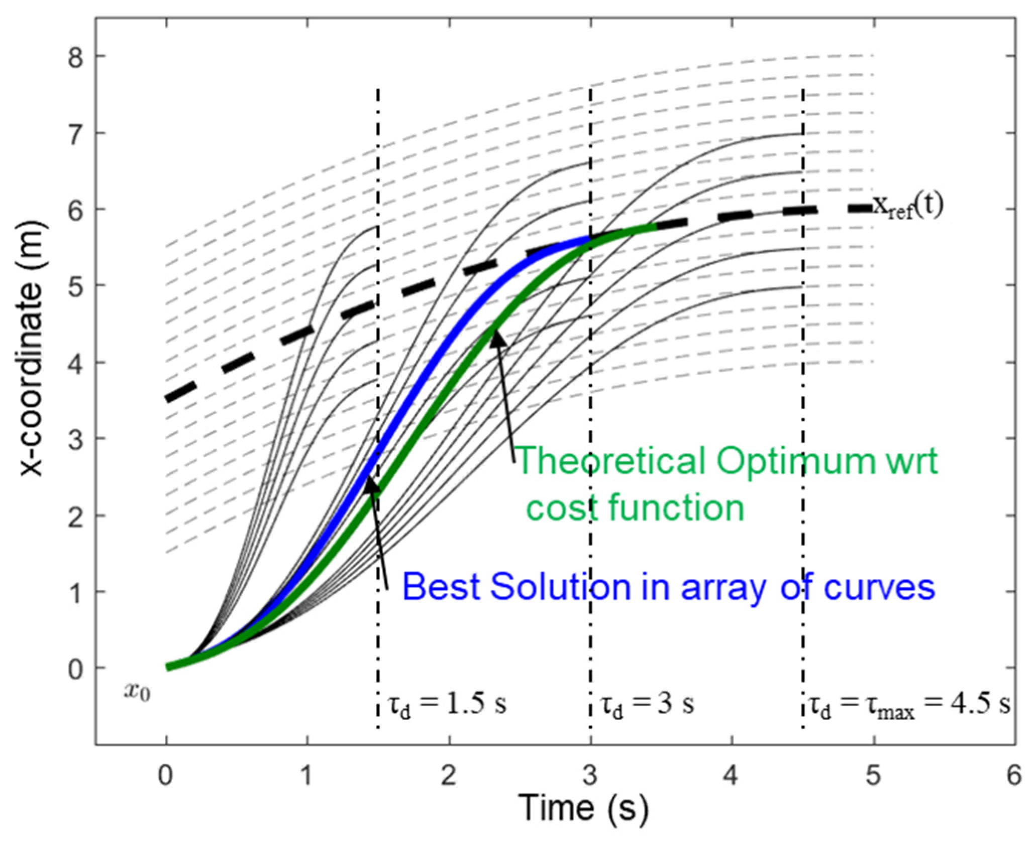
Figure 2 shows an example manifold of trajectories for a given reference curve x_ref.

Based on the cost function (3), the best trajectory within the manifold is selected, which is only an approximation of the theoretical optimum. The distance to the theoretical optimum depends on the selected resolution of the discretization.

In addition to the cost function, also boundary conditions (4–8) are considered, which are related to the physical feasibility of the trajectories.

$$\sqrt{a_x^2+a_y^2}\le a_{\max }$$

(4)

$$\left|\kappa \right|\le {\kappa }_{\max }$$

(5)

$$m{a}_x+F_{\mathrm{friction}}+F_{\mathrm{drag}}\le \frac{i}{r}{M}_{\mathrm{Engine},\max }$$

(6)

$$\left(m{a}_x+F_{\mathrm{friction}}+F_{\mathrm{drag}}\right)v\le P_{\mathrm{Engine},\max }$$

(7)

$$v\le v_{\max }$$

(8)

$$d_{\min }\le d\le d_{\max }$$

(9)

They include the limitation of total horizontal acceleration due to tire friction $a_{\max }$ (4), limit of curvature ${\kappa }_{\max }$ (5), limit of engine torque $M_{\mathrm{Engine},\max }$ together with the transmission ratio i and the wheel radius r (6), limit of engine power $P_{\mathrm{Engine},\max }$ (7) and speed limitation $v_{\max }$ (8). Boundary condition (9) makes sure that the vehicle does not leave the accessible width of the road. If one or more of these boundary conditions are violated, the trajectory is removed from the manifold. Furthermore, a collision check is performed with respect to the obstacle trajectories, and only collision-free trajectories, which satisfy pre-defined safety margins in space and time, are considered.

Trajectories are re-calculated with a pre-defined constant planning frequency. Within each time step, a manifold of trajectories is created and the best trajectory for a pre-defined time horizon is selected. As the initial state for the trajectory, the vehicle state according to the selected trajectory from the previous time step at the end of the current time step is used. With this new initial condition, a new manifold of trajectories is created. This manifold typically differs from the manifold from the previous time step because the end times τ of the trajectories are shifted by a time step. Thus, after each time step, a new optimal trajectory might be selected, which differs from the previously selected trajectory. The differences between selected trajectories of subsequent time steps are typically in the order of discretization resolution of the manifold. However, larger differences between subsequently selected trajectories occur if relevant changes in the planning scenario occur. This might be the case, if the predicted trajectory of an obstacle changes, if differing planning parameters are passed to the motion planner by a previous instance, or if the vehicle does not follow the intended trajectory with sufficient accuracy. For the latter case, thresholds of position deviation in lateral (b_lat) and longitudinal (b_long) directions are defined. If these thresholds are violated, a new trajectory is planned, which uses an initial position based on an extrapolation of the real vehicle movement instead of the previously planned trajectory.

2.2. Motion Controller

The task of the motion controller is to provide set points for the actuator management of the vehicle, which make the vehicle follow the trajectory provided by the trajectory planner. The used controller is a kind of nonlinear state-space controller. The controlled states for longitudinal dynamics are the velocity deviation Δv and the longitudinal position deviation Δs. For lateral dynamics, the lateral position deviation Δd and the deviation of the heading angle $\Delta \psi$ are considered. These controller deviations are computed based on the vehicle state, which the vehicle is currently supposed to have according to the planned trajectory. The lateral position deviation Δd is the perpendicular distance of the actual vehicle position to the vector, which is tangential to the trajectory at the location, where the vehicle is currently supposed to be. The longitudinal position deviation Δs is correspondingly the distance component parallel to this vector. The deviations of velocity and heading angle are computed as the difference between actual and planned value according to the trajectory for the current moment. The controller parameters corresponding to the four controlled states are k_v, k_s, k_d and $k_{\psi }$. The control laws are denoted in Equation (10) for longitudinal and Equation (11) for lateral dynamics.

$$a_{\mathrm{cont}}=a_{\mathrm{traj}}\left(s\right)+k_v\Delta v+k_s\Delta s$$

(10)

$${\kappa }_{\mathrm{cont}}=\frac{1}{{\kappa }_{\mathrm{rat}} (a_y,v)}\left({\kappa }_{\mathrm{traj}}\left(s\right)\frac{\cos \left(\Delta \psi \right)}{\left(1-{\kappa }_{\mathrm{traj}}\left(s\right)\Delta d\right)}-k_d\frac{\Delta d}{v^2}-k_{\psi }\frac{\sin \left(\Delta \psi \right)}{v}\right)$$

(11)

$$\frac{{\kappa }_{\mathrm{actual}}}{{\kappa }_{\mathrm{requested}}}\approx {\kappa }_{\mathrm{rat}} (a_y,v)=\min \left(1,{\kappa }_{\mathrm{rat},0}+c_{ay}\left|a_y\right|+c_v\left|v\right|\right)$$

(12)

In these equations, the acceleration $a_{\mathrm{traj}}$ and the curvature ${\kappa }_{\mathrm{traj}}$ correspond to the vehicle motion, which is currently intended by the trajectory planner. They represent the base of the controller output, to which modifications based on the state deviations are added. For controlling the longitudinal dynamics of the vehicle model described in Section 2.3, the linear control law in Equation (10) is sufficient. For the lateral control, the sensitivity of the curvature command ${\kappa }_{\mathrm{cont}}$ with respect to state deviations is decreasing with increasing velocity v in a way that keeps the time for compensating a given state deviation constant regardless of velocity. This makes the controller feasible for a larger velocity range.

Since the vehicle model does not follow the controller output ${\kappa }_{\mathrm{cont}}$ exactly, a pre-control is included, Equation (12). It compensates for the effect of understeering of the vehicle in a stationary state using a linearized function for the ratio ${\kappa }_{\mathrm{rat}}$ of actual and requested curvature as a function of velocity v and lateral acceleration a_y. The pre-control function is limited to a maximum value of one to avoid unrealistic higher values, which might occur due to linear extrapolation.

2.3. Vehicle Model

The vehicle model includes a vehicle dynamics sub-model with tires, sub-models of the actuators (i.e., powertrain, steering, and braking system), and a sub-model of the actuator management.

As shown in Figure 1, the actuator management receives the target signals of the longitudinal acceleration and curvature from the motion control. Within the developed actuator management model, these signals are translated into drive signals for the single actuators, by implementing simple algebraic transformations.

The drive signal of the longitudinal acceleration is used to compute the target powertrain and brake torques. To this aim, a simple point mass model for longitudinal dynamics is implemented, which considers basic powertrain and vehicle parameters (such as the torque-velocity characteristic, the maximum torque, the maximum power, and the wheel radius). The powertrain model implements a simplified rigid 1D rotational dynamics of the whole transmission from the motor up to the wheel inertias. To this aim, the actual powertrain torque is firstly obtained from the target torque, by implementing a simplified electric motor model based on look-up-tables and adding the other torque inputs of the system, such as the tire reaction torques, and the braking torques. As a result, the wheel rotational velocities and the reaction torques to the unsprung and sprung masses of the vehicle dynamics model are computed.

The braking model includes a stick-slip friction formulation of the braking torques, which depend on the actuator management demand, and on a first-order transfer function, which models the delay in the whole braking system.

For the lateral dynamics, the target curvature signal is transformed into the steering rack position, by considering a pure Ackermann steering in an ideal kinematic single-track model (i.e., neglecting tire slip), thus implementing a simplified steering system with no internal dynamics.

The output signals of the actuator models (i.e., the rotational velocity of the wheels, the reaction powertrain, and braking torques, and the steering rack position) are delivered to the vehicle dynamics model, which includes the vehicle chassis with suspensions and the tires. The chassis model is based on a reduced 3D multi-body approach. The sprung mass has 6 degrees of freedom (DOFs). This is connected via the suspension constraints to the two front unsprung masses (each of them with two relative 3D-spatial DOFs) and the two rear unsprung masses (each of them with one relative 3D-spatial DOF). Since the wheel rotations and the steering rack position DOFs are imposed as so-called motions, they do not account for the total number of DOFs of the system, which are then ten in total.

The suspension constraint represents a pure kinematic 3D constraint involving all six coordinates as a function of the displacement along the vertical coordinate z of the wheel center relative to the car body and of the steering rack displacement x_r (the latter just for the front axle). This can be written as

$$x_k=x_k\left(z,x_r\right),$$

(13)

where $x_k$ represent the vector of all translational and rotational coordinates of a single unsprung mass. In the same way, also the spring displacement and the damper velocity are obtained. These functions are modeled as look-up-tables or polynomial functions for better computational performance.

The suspension kinematic Equation (13) is combined with the dynamical equilibrium equations of the sprung and unsprung masses as well as the equation of force equilibrium along the suspension DOFs (involving the suspension loads and the spring, damper, and anti-roll bar forces). The resulting equation system is built after symbolic manipulation, so that the accelerations of the Lagrangian coordinates $q$ (i.e., the system DOFs) and the Lagrangian multipliers (i.e., the suspension loads $L_c$) can be obtained by solving the following linear problem

$$A\left(q,\dot{\mathbf{q}}\right)\left[\begin{array}{c}\ddot{q}\\ L_c\end{array}\right]=b\left(q,\dot{q,}{L}_t,L_a,T,{\mathsf{\omega }}_w,x_r,{\dot{x}}_r,{\ddot{x}}_r\right),$$

(14)

where $L_t$ represents the tire loads, $L_a$ the aerodynamic load, $T$ all torque inputs (from powertrain and braking system), and ${\mathsf{\omega }}_w$ the wheel rotation velocities.

The tire is implemented by means of the Magic Formula tire model by Pacejka [17] for the horizontal forces and the three moment components. The vertical tire force is obtained by a spring-damper equivalent system, which represents the tire vertical compliance. This allows the model to simulate the main effects of the tire interaction with uneven road profiles, even if with a simplified approach. The tire slip dynamics is modeled with a dynamic system of the first order depending on the tire relaxation length parameter. To overcome the well-known numerical problem of the tire slip formulation at a speed close to zero, the equations of the slip dynamics are implemented with the modification suggested in [18], which allows the vehicle to fully stop and restart.

In the presented vehicle model, an additional feature was implemented, to model the behavior of active suspensions. This includes an external interface to receive the signals of the suspension actuator forces as input from the active suspension controller model. These force signals are then added to the equilibrium of the suspension along its DOF, together with the suspension loads and the spring, damper, and anti-roll bar forces.

The level of detail of the proposed vehicle model is suitable for vehicle dynamics simulations in the application fields of handling and low-frequency comfort.

3. Application Example: Test of an Active Suspension Control System

As an application example for the model chain described in Section 2, the test of an active suspension control system is discussed in this section. The test objectives are to verify the functionality of the subsystem, especially with respect to the collaboration with a dynamical replanning trajectory planner, the quantification of the effect on driving comfort, and the analysis of the effect of the active suspension system on the lateral and longitudinal vehicle motion, which is controlled by the motion controller described in Section 2.2. The active suspension control system is described in Section 3.1, the test scenario and the simulation results are shown in Section 3.2.

3.1. Description of the System under Test

The principle of vertical trajectory planning for active suspension control of automated vehicles has been introduced in previous publications [14,19]. It enables optimal control of roll-, pitch, and heave motion with regard to passenger comfort. Therefore, the optimal vehicle motion is derived as an optimization problem. Latter is defined as a function of the vehicle’s trajectory, the physical limitations of the suspension, and a cost function that determines what is optimal.

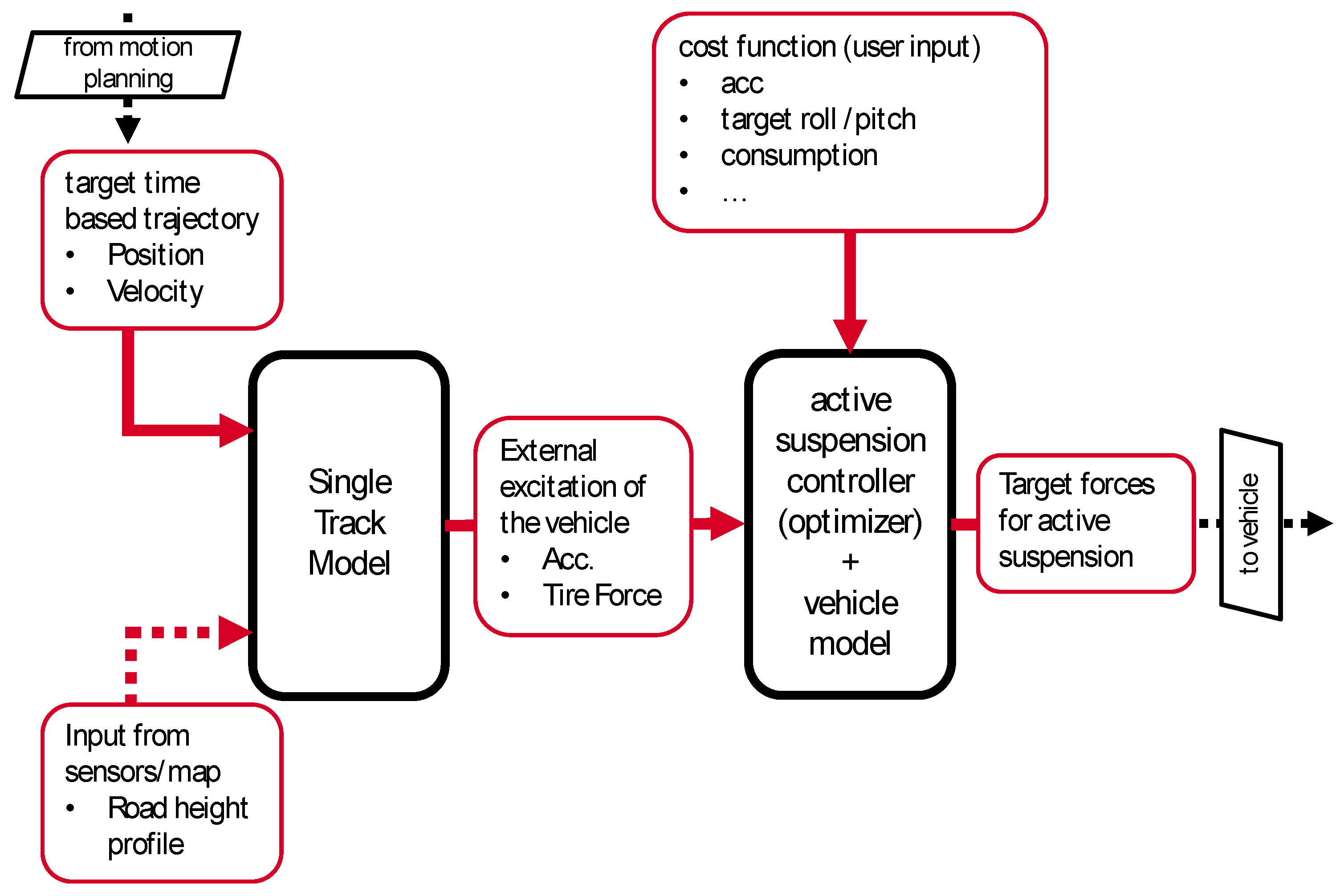
Figure 3 shows the structure of the active suspension controller.

In the first step, a single-track model is used to derive the external excitation of the vehicle. Latter is determined through the future (target) trajectory and road excitation, which can be obtained using environment sensors such as a stereo camera or LIDAR, or out of a digital map. As the control values are highly dependent on the inputs, the input signals have to be checked for plausibility to deactivate the controller in case of, e.g., discontinuities. The preview-information of external vehicle excitation is then used as input for the active suspension controller. Inside the active suspension controller, an optimization problem is set up to find the four optimal target forces (one for each corner), which lead to the desired optimal vertical motion. The resulting optimization problem is given in Equation (15):

$$\begin{array}{l}\underset{\overrightarrow{x}}{\min }f\left(\overrightarrow{x}\right)\\ \mathrm{with}:\overrightarrow{x}={\left[{\overrightarrow{F}}_1,{\overrightarrow{F}}_2,{\overrightarrow{F}}_3,{\overrightarrow{F}}_4,\overrightarrow{z},\overrightarrow{\phi },\overrightarrow{\theta },\overrightarrow{\dot{z}},\overrightarrow{\dot{\phi }},\overrightarrow{\dot{\theta }}\right]}^T\end{array}$$

(15)

where F_x denotes the actuator force at the four corners of the vehicle and z, $\phi$ and $\theta$ are roll, pitch, and heave motions as well as their derivatives. Optimality is described in a flexibly adjustable cost-function f. Currently implemented criteria are body accelerations, -velocities, and -angles, as well as energy consumption of the active suspension, and both lateral and longitudinal acceleration experienced by the passengers. The optimizer uses a 3-DOF (roll, pitch, and heave)-model to calculate body motion as a function of external excitation and chassis component models. These are implemented through simplified component models such as spring characteristics.

Due to the lack of an appropriate simulation environment for automated driving including a trajectory planning algorithm, the vertical trajectory planner has been tested only in offline mode with a predefined trajectory until now. However, as in real-world driving trajectories change dynamically due to, e.g., interaction with other road users, the chassis controller must be capable to deal with dynamic input trajectories.

Therefore, a continuous, online version of the vertical trajectory planner has been derived. Following changes were necessary: The planning horizon is reduced to ~150 m with a resolution of 1–1.5 m, which results in a significant reduction of optimization variables and enables real-time capability with a mean calculation time lower than 0.1 s. For the simulation, the controller runs at 10 Hz.

For further reduction of calculation time, the optimizer uses the solution of the last iteration as a starting solution for the following iteration. As the input (target) trajectory usually does not change significantly between two iterations, the previous solution is an appropriate starting solution. If there is no change in the input trajectory, the optimization is skipped.

To avoid discontinuities between target forces of consecutive iterations, the initial state (roll, pitch, heave, and actuator force) must be constrained with regard to the previous iteration.

The target forces are sent to the vehicle dynamics and actuators model.

By adjusting the cost-function parameters, different vehicle characteristics can be implemented. To display the functionality, we used the following three setups for the simulations:

• Full roll- and pitch compensation: Both roll- and pitch angles are fully compensated by the active suspension. This leads to minimal rotational acceleration.
• Predicted curve tilt: The vehicle is tilted actively into the curve to enable compensation of lateral acceleration. As fast roll movements are uncomfortable, tilting speed is actively reduced by starting the tilt process slightly before entering the curve.
• Predictive curve tilt and helicopter: Variant predictive curve tilt with additional compensation of longitudinal acceleration by active pitch motion. Hence, the vehicle tilts backward while braking and forwards while accelerating.

3.2. Test Scenario for Simulation

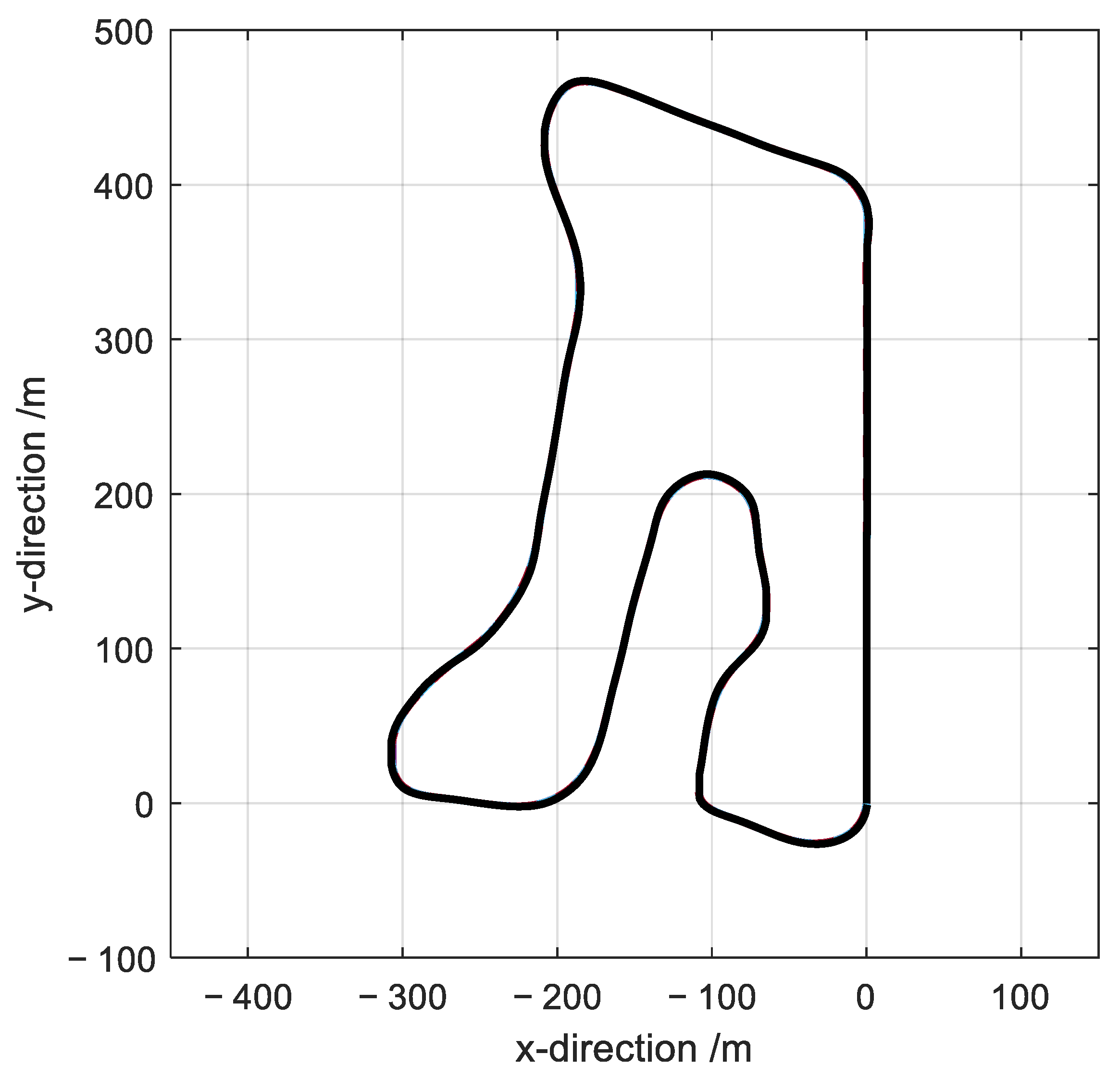
For testing the active suspension control system described in Section 3.1, a handling course is used as a test scenario, which is depicted in Figure 4.

The test track has a length of 1811 m. Its curvature values for each location are depicted in Figure 5a.

The narrowest curve occurs after a traveled distance of 1685 m with a curvature of κ = 0.0835 1/m, which corresponds to a curve radius of 12 m. In this and in the following figures, the traveled distance s is defined from the starting position x = y = 0 (see Figure 4), where the vehicle starts in a positive y-direction with an initial velocity of v = 0.

For the tests, two different scenarios are used: in the first scenario, a maximum resulting horizontal (longitudinal and lateral) acceleration of a_max = 0.25 g = 2.45 m/s² is allowed for the trajectories computed by the trajectory planner. This corresponds to a comfort-oriented driving, which is the normal driving mode of an autonomous vehicle. To also have a more challenging scenario for the system under test, a second test scenario with a higher allowed maximum resulting horizontal acceleration of a_max = 0.7 g = 6.87 m/s² is also analyzed. Such higher acceleration values may occur in suddenly changing traffic situations, where fast reactions of the autonomous vehicle are necessary, and safety becomes more important than ride comfort. The value of a_max = 0.7 g is chosen here because it is the corner case of the motion controller with the selected parameters (see

Table 1. Used parameters for simulation of the test cases.

Parameter	Symbol	Value
Trajectory planner
Planning frequency	fTrajectory	10 Hz
Prediction horizon for trajectory planning	τmax	7 s
Weighting factor for time to reach the longitudinal position	$w_{\tau s}$	1
Weighting factor for difference to desired velocity	wv	105
Weighting factor for time to reach the lateral position	$w_{\tau d}$	1
Weighting factor for lateral difference to reference curve	wd	1010
Lateral position threshold for trajectory replanning	blat	0.4 m
Longitudinal position threshold for trajectory replanning	blong	1.0 m
Maximum curvature	${\kappa }_{\max }$	0.165 1/m
Maximum traction force	$\frac{i}{r}{M}_{\mathrm{Engine},\max }$	7.5 kN
Maximum engine power	PEngine,max	77 kW
Maximum vehicle velocity	vmax	50 m/s
Motion Controller
Controller gain for longitudinal position deviation	ks	1.333
Controller gain for velocity deviation	kv	2
Controller gain for lateral position deviation	kd	4
Controller gain for heading angle deviation	$k_{\psi }$	4
Pre-control parameter	${ \kappa }_{\mathrm{rat},0}$	1.0585
Pre-control parameter for lateral acceleration dependency	cay	0.0049
Pre-control parameter for velocity dependency	cv	−0.0157
Low pass filter cut-off frequency	fcut	30 Hz
Vertical trajectory planner
Length of prediction horizon	N	7 s
Planning frequency	fVTP	10 Hz
Maximum actuator force	Fmax	10 kN
Maximum actuator travel	zmax	±40 mm
Vehicle
Wheelbase	l	2.924 m
Front track	t1	1.630 m
Rear track	t2	1.617 m
Distance of center of gravity from front axle	a1	1.496 m
Height of center of gravity	hG	0.522 m
Rolling radius of front tires	r1	0.316 m
Rolling radius of rear tires	r2	0.316 m
Mass	m	2150 kg
Sprung mass	ms	1990 kg
Single unsprung mass front axle	mu,1	40 kg
Single unsprung mass rear axle	mu,2	40 kg
Roll moment of inertia	Jxx	417 kgm2
Pitch moment of inertia	Jyy	1344 kgm2

). This acceleration at the vehicle’s center of gravity leads to an exploitation of the tire friction force potential of more than 90% at individual tires in simulation with the passive vehicle.

The velocity profiles computed by the trajectory planner for both cases are depicted in Figure 5b. It shall be noted that in most situations, the trajectory planner does not make full use of the allowed acceleration limits due to the given target function and other planning constraints (Equations (4)–(10)). The planned trajectories are also allowed to leave the given reference curve shown in Figure 4 if the lane width given by d_min and d_max is respected. However, with the weighting factors used for the trajectory planning, the planned trajectory typically follows the reference curve exactly in the given test cases (one exception will be discussed later in this section). The used simulation parameters for the tests are listed in Table 1.

3.3. Simulation Results

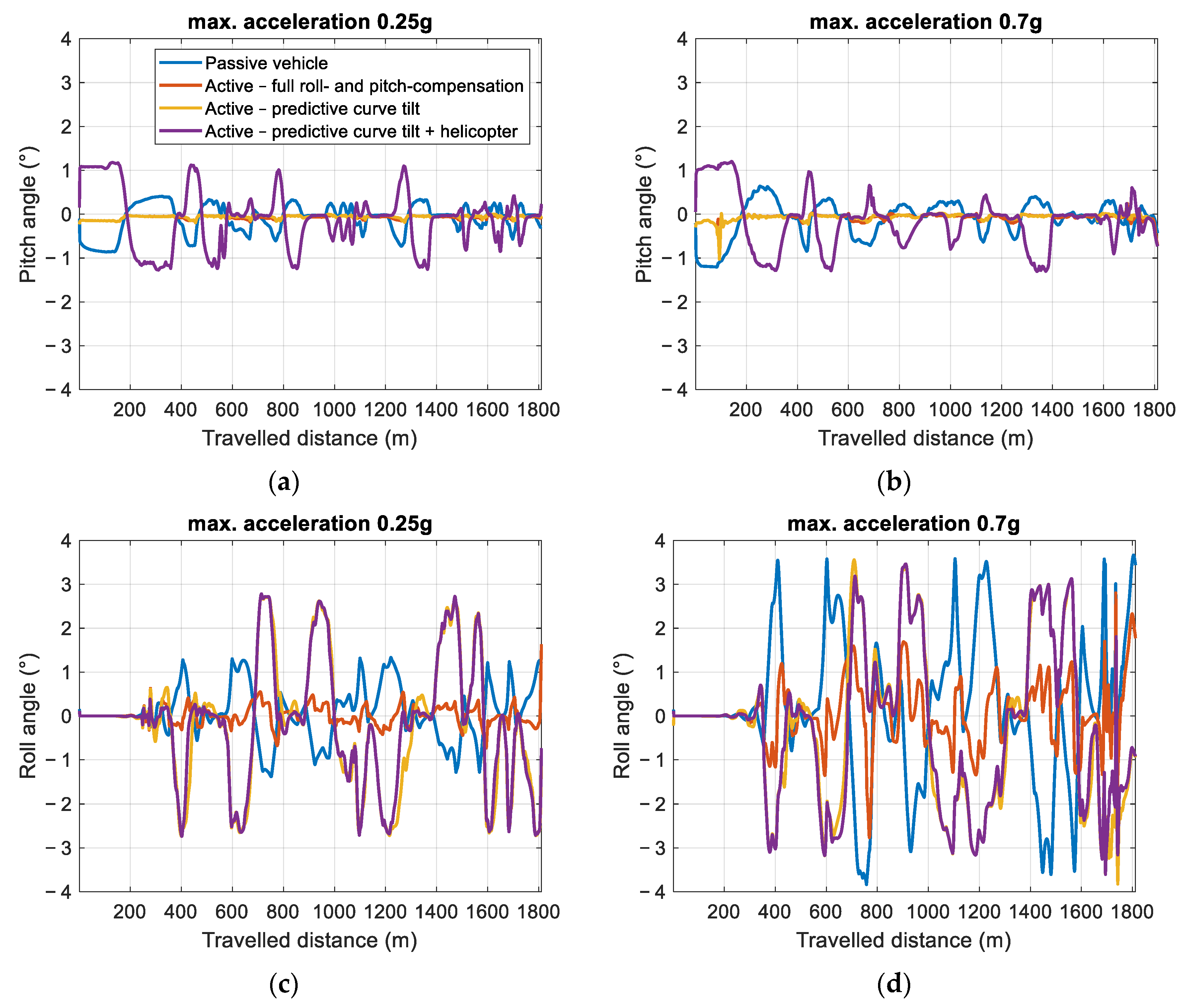
Figure 6 shows the vehicle roll- and pitch angle for the two cases “max. acceleration 0.25 g” and “max. acceleration 0.7 g”.

All simulation runs were carried out with the same vehicle model. The passive vehicle has conventional springs, dampers, and anti-roll bars. For the simulation of the active variants, the anti-roll bars are removed as the required forces for roll compensation are applied by the active system. The simulation results show that the passive vehicle compensates squat well while there is a brake dive of 0.5° in both cases. All the active variants do overcompensate the pitch motion. Both “full roll-and pitch compensation” and “predictive curve tilt” do not penalize longitudinal acceleration in the cost function, however, squat motion is slightly overcompensated (positive pitch angle while accelerating). Brake dive is fully compensated. “Predictive curve tilt and helicopter” leads to pitch angles of up to 2° for both accelerating and braking. Therefore, resulting longitudinal acceleration can be reduced.

With the passive vehicle, the roll angle is between −1.5 and 1.5° for the “max. acceleration 0.25 g” scenario and −4 and 4° for the more dynamic “max. acceleration 0.7 g” scenario. With “full roll- and pitch-compensation” roll motion can be reduced to near zero. As the complexity of the internal vehicle model in the vertical trajectory planner is limited to ensure real-time capability, full roll compensation cannot be achieved for the more dynamic scenario. However, roll motion is still reduced substantially when compared to the passive vehicle.

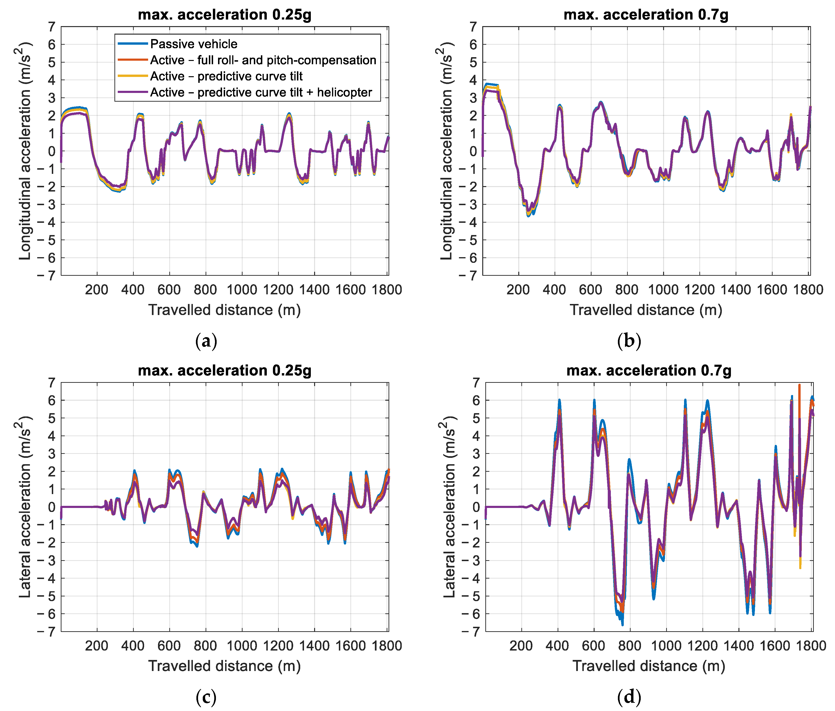
The resulting longitudinal and lateral accelerations, which are acting on the occupants are displayed in Figure 7. These simulation results show that by the active pitch motion, the longitudinal acceleration can be reduced by about 0.5 m/s² while accelerating (a_x > 0) and 0.3 m/s² while braking (a_x < 0). With the higher accelerations in the “max. acceleration 0.7 g”-scenario, relative differences are smaller. However, it can be expected, that typical maneuvers will not exceed 3 m/s² longitudinal acceleration with automated vehicles [3]. Therefore, the maximum longitudinal acceleration can be reduced by up to 20% in normal driving conditions.

For the lateral acceleration, the reduction is symmetrical in both directions. Variant “full roll- and pitch-compensation” achieves approximately 0.2 m/s² less acceleration while both curve tilting variants achieve a 0.7 m/s² reduction. Due to the smaller amplitude, the gradient, and therefore the roll velocity, can also be reduced.

In addition to the effect of the active suspension on the ride comfort, the simulations show an effect on the lateral vehicle dynamics, especially at high lateral accelerations. At the curve shown in Figure 8, the motion controller with the parameters given in Table 1 is not able to follow the reference curve with an accuracy that satisfies the replanning threshold of b_lat = 0.4 m lateral distance for the scenario of the maximum allowed horizontal acceleration of 0.7 g. For this scenario, tire slip non-linearity has a significant effect on vehicle dynamics, but the motion controller is not designed for such nonlinear vehicle behavior.

Thus, the trajectory planner plans a new trajectory, which is no longer on the reference curve. This interactively replanned trajectory is also depicted in Figure 8 as a dotted line. Here only the currently desired position of the trajectory planner is plotted, but not any planned positions for the future. The replanning events occur as steps in the trajectory. With the active suspension system, the vehicle motion is supported in a way that enables a narrower curve radius satisfying the lateral position threshold. In this case, no replanning takes place, and the planned trajectory is always on the reference curve. Obviously, the effect is stronger the more the vehicle body is tilted towards the inner side of the curve, so predictive curve tilt has a stronger positive effect than roll compensation.

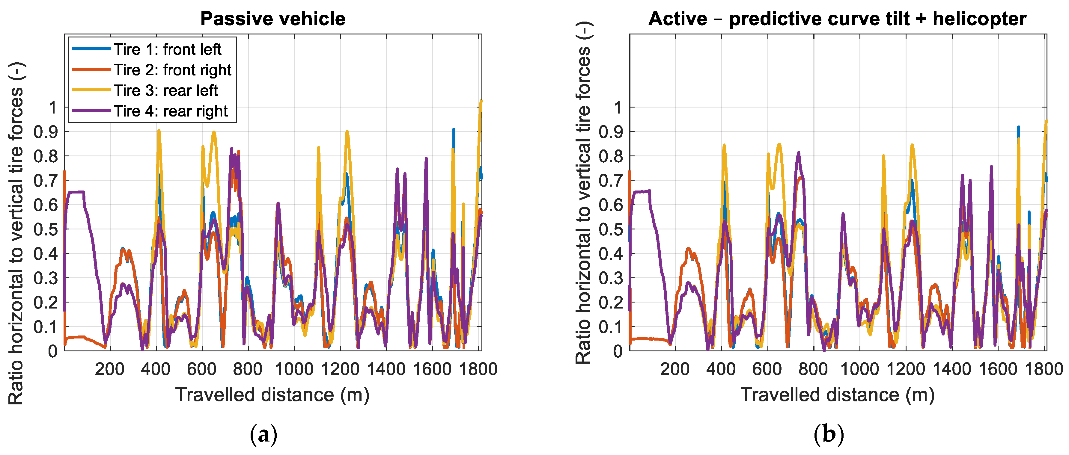
Figure 9 depicts the ratio of the horizontal tire forces (resulting from lateral and longitudinal forces at the contact point to the road) to their theoretical maximum (which is the product of the vertical tire force and the friction coefficient, which is equal to one in these simulations). The comparison between the active and the passive suspension shows that the tire force reserve is increased by the active suspension system in several driving situations along the handling course.

4. Conclusions

This paper shows the benefit of analyzing trajectory planning, motion control, and vehicle dynamics including the active suspension system in a closed-loop simulation. Whilst the active suspension uses information about the planned trajectory, the trajectory planner may react to the vehicle motion, which is influenced by the active suspension. This interaction shows the need to have a detailed vehicle model including the active suspension system. This can also be relevant for other test cases than the one discussed in this paper. For example, optimization of the motion controller parameters may give different results when using the active suspension system in the simulation rather than without using it.

From the perspective of the active suspension control algorithm, it was shown that the closed-loop simulation offers the possibility to test the integration with the automated driving function in an early stage of development and with low cost compared to the integration into a prototype vehicle. The results prove that the vertical trajectory planner works properly in interaction with dynamically changing input trajectories. Scopes of further research with regard to a potential series implementation are the development of a safety concept with a fallback solution in case of, e.g., non-plausible input values or failed optimization, as well as further adjustment of cost-function parameters to increase ride comfort.