Article

Modern Optimal Controllers for Hybrid Active Power Filter to Minimize Harmonic Distortion

1
Department of Electrical Engineering, Faculty of Engineering, The Hashemite University, P.O. Box 330127, Zarqa 13133, Jordan
2
Protection and Metering Department, National Electric Power Company, Amman 11181, Jordan
3
Department of Electrical Engineering, Faculty of Engineering, Mutah University, Mutah, AlKarak 61710, Jordan
4
School of Science, Engineering & Environment, University of Salford, Salford M5 4WT, UK
5
Department of Electrical and Electronics Engineering, New Horizon College of Engineering, Bangaluru 560087, India
6
School of Engineering, Edith Cowan University, Joondalup, WA 6027, Australia
*
Author to whom correspondence should be addressed.
Electronics 2022, 11(9), 1453; https://doi.org/10.3390/electronics11091453
Submission received: 30 March 2022 / Revised: 23 April 2022 / Accepted: 29 April 2022 / Published: 30 April 2022
(This article belongs to the Section Power Electronics)

Abstract

:
Nowadays, AC distributed power networks are facing many challenges in guaranteeing and improving the required level of power quality indices in power networks with increasing nonlinear, time-variable and unbalanced loads. Power networks can benefit from avoiding and minimizing different AC problems, such as frequency fluctuation and Total Harmonic Distortions (THDs), by using power filters, such as Hybrid Active Power Filters (HAPFs). Therefore, attention towards responsible power quality indices, such as Total Harmonic Distortion (THD), Power Factor (P.F) and Harmonic Pollution (HP) has increased. THD and HP are important indices to show the level of power quality at the network. In this paper, modern optimization techniques have been employed to optimize HAPF parameters, and minimize HP, by using a nature-inspired optimization algorithm, namely, Whale Optimization Algorithm (WOA). The WOA algorithm is compared to the most competitive powerful metaheuristic optimization algorithms: Manta Ray Foraging Optimization (MRFO), Artificial Ecosystem-based Optimization (AEO) and Golden Ratio Optimization Method (GROM). In addition, the WOA, and the proposed modern optimization algorithms, are compared to the most competitive metaheuristic optimization algorithm for HAPF from the literature, called L-SHADE. The comparison results show that the WOA algorithm outperformed all other optimization algorithms, in terms of minimizing harmonic pollution, through optimizing parameters of HAPF; therefore, this paper aims to present the WOA as a powerful control model for HAPF.

1. Introduction

1.1. Background

Recently, electrical energy consumption has increased worldwide, due to the increase in population and the electrification of industrial processes, such as vehicles, and new customers’ behavior in observing rapid technological progress. Therefore, attention towards responsible energy utilization and high-power quality indices has increased [1,2]. Power networks benefit from avoiding and minimizing different AC problems, such as frequency fluctuation and THD [2]. However, AC distributed power networks have faced many challenges in guaranteeing and improving the required level of power quality indices, with increasing nonlinear loads [3,4]. In the last few years, there has been an increase in interest in improving the efficiency of power filters to improve devices and network performance. This process is described in [5,6] as a complex and challenging optimization problem. In this work, the proposed new optimization algorithms have been tested and employed to achieve optimal performance in terms of power quality.

1.2. Literature Review

In general, nonlinear load is caused by two main types of harmonic distortions: current and voltage harmonic sources [5,6,7]. In addition, non-linear loads lead to lower power factors, higher power transmission-line losses and higher Total Harmonic Distortions (THDs). In power systems, minimizing the THD is an important and main task in improving the power quality of the electrical system. In the last few years, power filters have been studied and used to minimize the THD from the power grid. In general, there are three main types of power filters: Passive Power Filter (PPF), Active Power Filter (APF) and Hybrid Active Power Filter (HAPF) [5]. However, the disadvantage of using PPFs in the power network is limited ability to follow the dynamic behavior of nonlinear loads. To overcome this problem, APF has three-phase Pulse Width Modulated (PWM) included and uses voltage source inverters, which have more efficiency, less cost and less size compared to current source inverters [5,6,7]. APFs need a high level of power rating compared to PPFs [8]. Therefore, HAPFs have been introduced as a solution that have the benefits of APF and PPF due to combining them [5,8].
In the literature, many studies have concentrated on controlling PPF by using different optimization algorithms, such as Particle Swarm Optimization (PSO) and direction hybrid [9,10]. However, the literature [8,9,10] focused on using a common control method (PWM) [8], and developing optimal control for power filters based on a common optimization algorithm (PSO) [9,10]. The results in [9,10] did not consider the significance of using modern optimization algorithms. Therefore, developing and employing new and powerful metaheuristic optimization algorithms, such as WOA, can be beneficial for improving the power quality performance in the network. There is a limited number of studies on designing HAPF-based metaheuristic optimization algorithms, due to the complexity of the model. For example, the authors in [8] have used the L-SHADE optimization algorithm to improve HPAF. However, the L-SHADE optimization algorithm has only been compared to a common algorithm, such as the Differential Evolution (DE) algorithm. In addition, to the best of the authors’ knowledge, there is no work on HAPF that has been addressed by using these modern optimization algorithms and which include a comprehensive comparative case study for the optimization algorithms. In this paper, modern optimization techniques have been employed on HAPF to minimize the THD and improve the power quality at power networks. The modern optimization techniques in this work are: Whale Optimization Algorithm (WOA) [11], Manta ray foraging optimization (MRFO) [1,12], Artificial Ecosystem-based Optimization (AEO) [13] and Golden Ratio Optimization Method (GROM) [14,15]. These modern optimization algorithms have been compared to the following powerful, and most competitive, metaheuristic optimization algorithms: Autonomous Groups Particles Swarm Optimization (AGPSO), Modified Particle Swarm Optimization (MPSO), Improved Particle Swarm Optimization (IPSO) [16], Equilibrium Optimizer (EO) [17,18] and L-SHADE optimization algorithm [8]. Among modern optimization techniques, the WOA has a great deal of experience in solving complex engineering optimization problems [11,19]. The obvious advantages, such as simplicity, flexibility, fast convergence speed, and stochastic nature, have attracted considerable interest from the current research community in a variety of fields, including electrical and power systems, data mining and machine learning, and wireless sensor networks [19,20]. Therefore, this paper aims to present the WOA as a powerful control model for HAPF parameter optimization.

1.3. Contributions

In this work, the proposed optimization algorithm, WOA, has been evaluated on two configurations of HAPF. The first configuration included the APF and the shunt passive filter in series with non-linear load and source. In the second configuration, the APF and the shunt passive filter were combined and connected with non-linear load and source. In both configurations, the THD problem in HAPF was formulated as a single objective function [5,8]. The proposed optimization algorithms were applied in this work to minimize voltage and current THD at the same time. In general, a limited number of researchers [8] have focused on applying common optimization algorithms to solve the THD problem in HAPF. Achieving the minimum THD for HAPF is a complex and challenging task. Therefore, it is important to employ more flexible and modern optimization algorithms. The main contributions of this paper can be summarized as follows: firstly, a new optimization algorithm, WOA, is applied and employed to improve the performance of HAPF; secondly, a comprehensive comparative case study is conducted for the proposed modern optimization algorithms (MRFO, AEO, GROM) and the common powerful optimization methods from literature (AGPSO, MPSO, IPSO, EO, L-SHADE). To the best of the author’s knowledge, there is no work on HAPF that has addressed using these modern optimization algorithms.

1.4. Outline of Paper

The remainder of this article is organized as follows: the circuit system of HAPF and the optimization problem are introduced in Section 2; the optimization process and WOA algorithm are presented in Section 3; case studies and results of the proposed optimization models are discussed in Section 4 and Section 5; and, finally, the conclusions and summary of this work are presented in Section 6.

2. Methodology

In this article, HAPFs are used to improve the power quality of power circuits. In power systems, minimizing HP and THD are significant factors in improving power quality of the electrical system. However, to achieve higher power quality, it is necessary to optimally control the HAPF. In this work, different modern optimization algorithms are evaluated on two configurations of HAPF. The outline scheme of the HAPF optimal controlling process is:
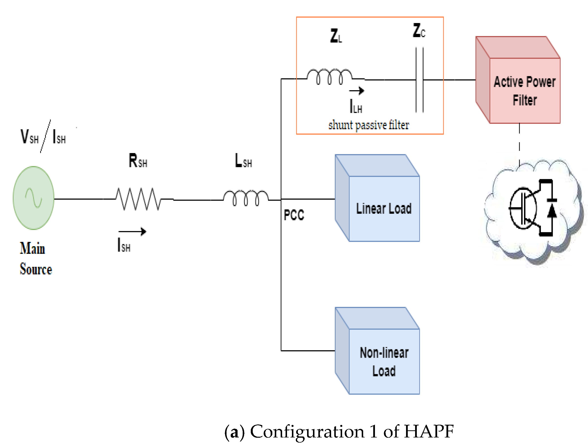
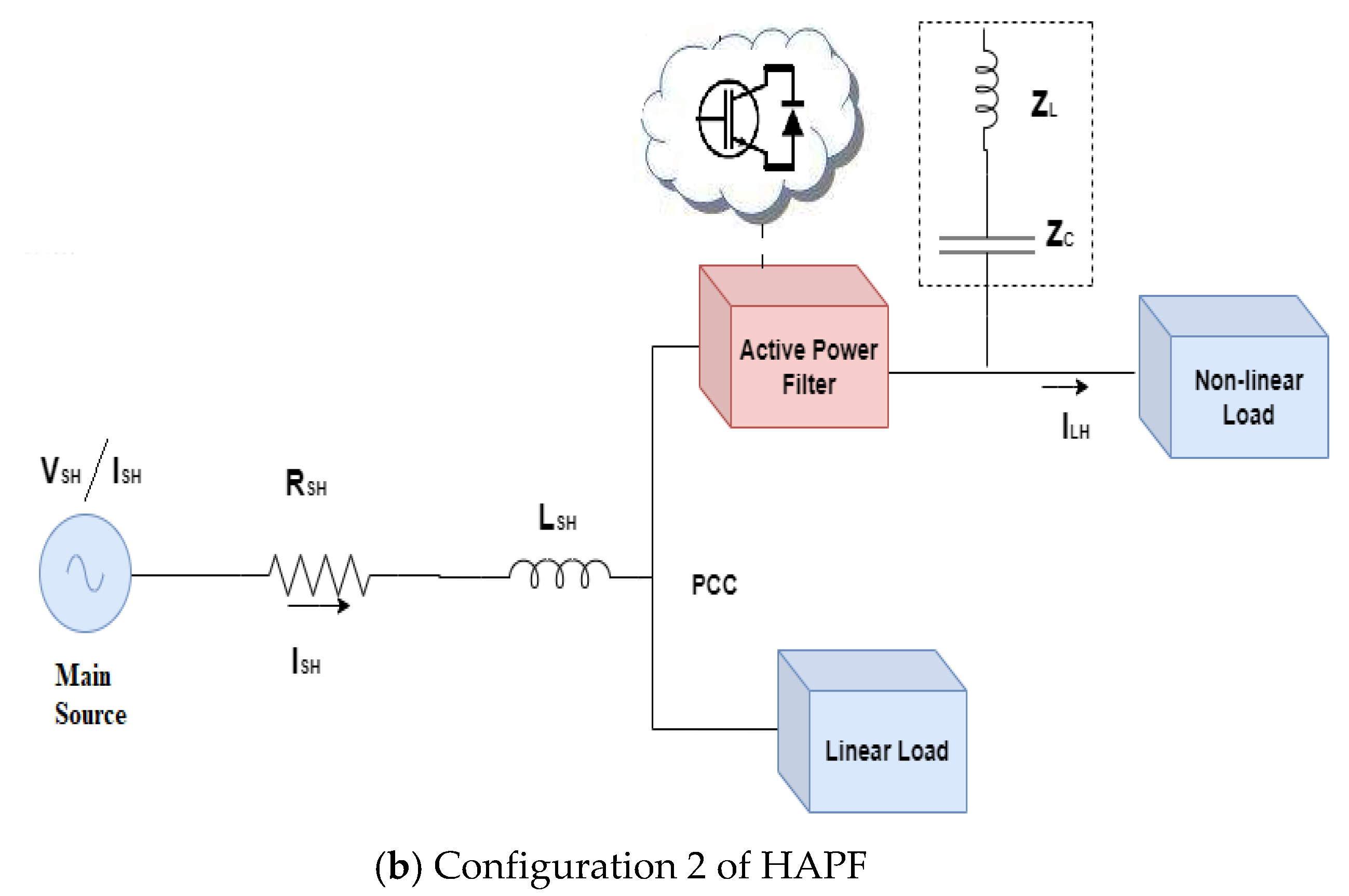
  • Firstly, the topology of HAPF and the problem statement are described. In Section 2.1, the description of the HAPF, based on two configurations, is presented. Based on the topology of HAPF, the power quality problem has been described as an optimization problem under a number of constraints.
  • Secondly, the HAPF optimization problem has been solved by using different optimization algorithms. Section 3 presents the methodology of the optimization algorithms to solve the HAPF optimization problem.

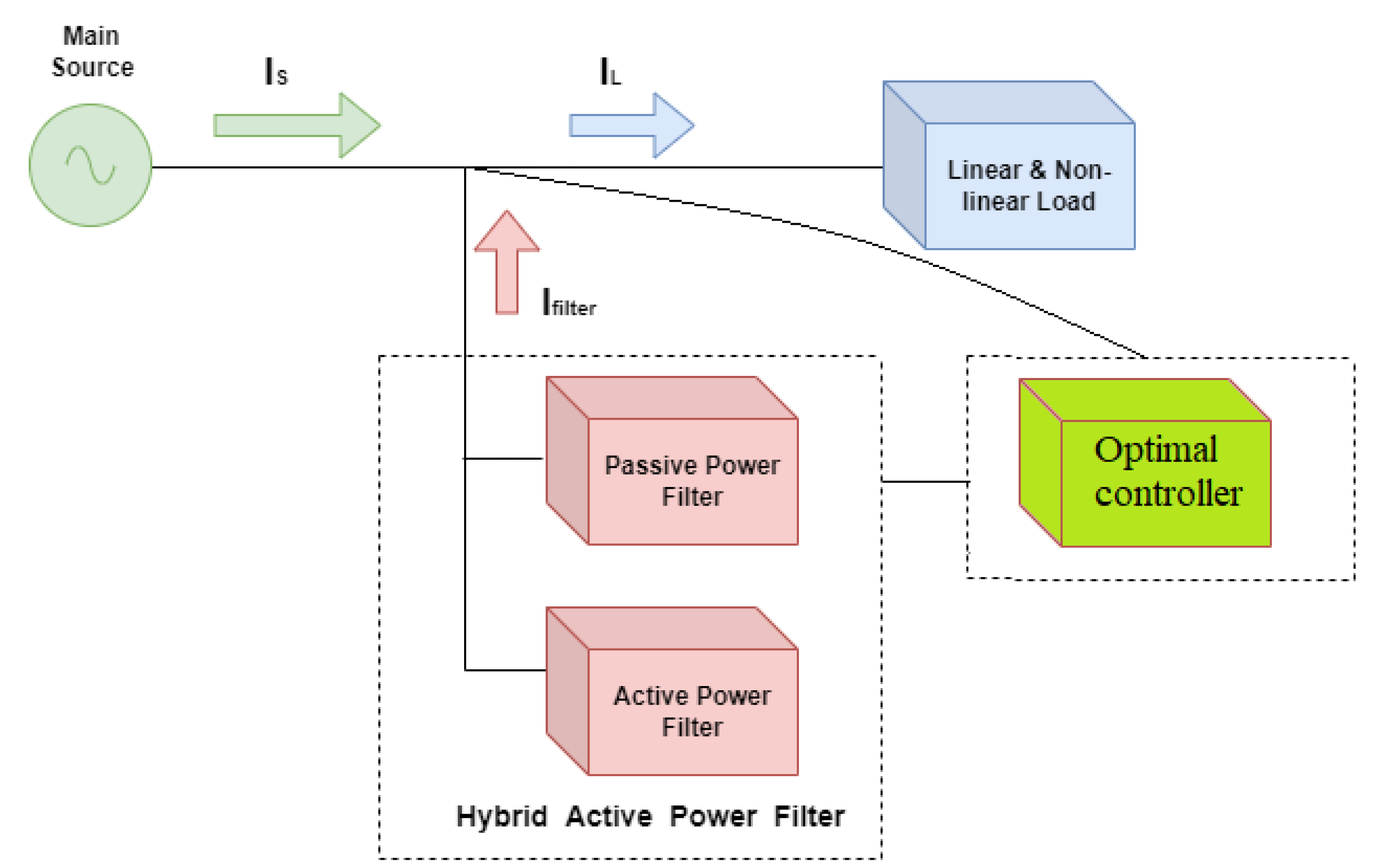
2.1. System Description and Problem Statement: Hybrid Active Power Filters

The basic topology of HAPF for the system is shown in Figure 1. This system consists of a power supply (voltage source), HPAF and a nonlinear load. As previously discussed, HAPF is mainly the combination of PPF and APF [8,19].
In this work, two configurations of HAPF are commonly used in power systems. Figure 2a presents the first configuration of HAPF, where the APF and the shunt passive filter are in a series with a nonlinear load and source. In this configuration, the APF injects a harmonic compensation current to cancel the load harmonic and improve the performance of PPF. In addition, the dropped voltage over the PPF will also reduce the voltage rating of the APF [5]. In the second configuration, as shown in Figure 2b, the APF and the shunt passive filter are combined. This configuration allows a lower rating of current in the APF, due to high impedance at the series APF. In Figure 2, the point of common coupling (PCC) represents the point where the load is connected to the system. The PPF is represented by inductive,   Z L , and reactance, Z C , as tuned filter, as shown in Figure 2. The voltage and current source, transmission line resistance and reactance and load current at the harmonic, H, are presented by V SH , I SH , R SH ,   L SH and I LH   , respectively. To minimize the voltage THD, APF works as a controlled voltage source. The APF injects a voltage harmonic waveform to cancel the voltage THD in the system. The voltage harmonic waveform is equal to the proportional factor, F, of the harmonic current. In this work, the proposed optimization method aimed to find the optimal values of F, Z L , and Z C under both configurations so as to achieve the minimum impact of THD [5,8].
In general, HAPF combines both APF and PPF to reduce the size and cost of the filter compared to APF. HAPF, under the main two topologies, shown in Figure 2, is normally used for compensation in industrial power systems. This compensation is worked without indicating the interface transformer at the power system [5,6,7,8]. In the power system, the PCC is the closest point to the load and is identified as the point where the load is connected to the power system. This common power system structure will help controllers achieve synchronization with the grid voltage, as presented in [2,5,8]. In addition, common control strategy and power transformation, to compensate for currents, voltages and power, are based on the synchronous reference frame detection method as described in [2] and used in [2,5,8].
In this work, the impact of THD on the power system is represented by Harmonic Pollution (HP) as per [21]. In power networks, the higher the level of HP, the greater the potential risk, installation and power quality problems at the power network. The HP is described by Equation (1)
HP = VTHD 2 + ITHD 2
where the VTHD and ITHD are the voltage and current THD, respectively. The F, Z L , and Z C as decision variables are then used to minimize HP by minimizing VTHD and ITHD. The description of the common and known VTHD and ITHD equations is prescribed by IEEE 519-2014 [22]. Equation (2) describes the optimization problem in this work.
arg   min F ,   Z L ,   Z C   HP
Subject to the following:
  • HAPF parameters [8,22].
0 F 20
0 Z L 10
0 Z C 10
  • The VTHD and ITHD limitation ( VTHD lim , ITHD lim ) based on IEEE 519-2014 [22].
VTHD VTHD lim
ITHD ITHD lim
  • Power factor limitation [8,22].
    PF = PF target + ε
    where the power factor in the network, PF, needs to be equal to the target power factor with a small error, ε , less than 10 2 .

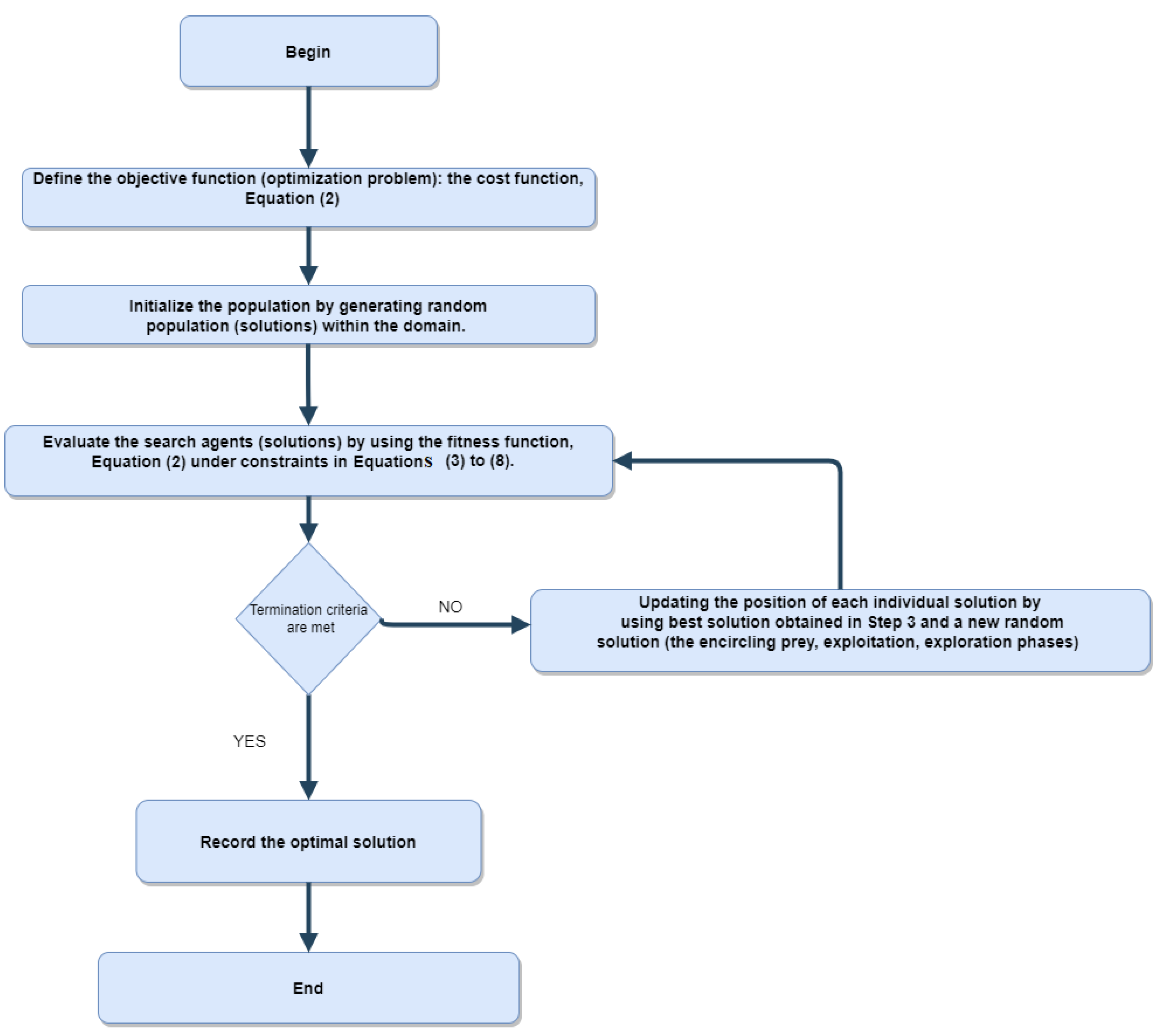
3. Description of the Modern Optimization Algorithms

The optimal operation of HAPF requires minimization of HP by selecting optimal decision variables F, Z L , and Z C to reduce VTHD and ITHD. The objective function, as described in Equation (2), is designed to minimize HP by considering the optimal values of F, Z L , and Z C under several constraints, Equations (3) to (8). In this study, the proposed WOA is considered to optimize the parameters of HAPF, and the results of the proposed WOA are compared with other modern optimization algorithms, such as MRFO, AEO, and GROM.
Modern optimization algorithms are employed and applied in this work to find and achieve the minimum HP: Whale Optimization Algorithm (WOA) [11], Manta ray foraging optimization (MRFO) [1,12], Artificial Ecosystem-based Optimization (AEO) [13] and Golden Ratio Optimization Method (GROM) [14,15]. These modern optimization algorithms were used to solve complex and stochastic optimization problems in the simplest way within a low computational. In addition, the results of the proposed WAO optimization algorithm were compared to powerful, and most competitive, metaheuristic optimization algorithms, namely: Autonomous Groups Particles Swarm Optimization (AGPSO), Modified Particle Swarm Optimization (MPSO), Improved Particle Swarm Optimization (IPSO) [16], Equilibrium Optimizer (EO) [18,21] and L-SHADE optimization algorithm [8]. From the results of the analysis, it is shown that the WOA algorithm outperformed all other optimization algorithms in terms of minimizing HP. Therefore, this paper aims to present the WOA as a powerful control model for HAPF. The WOA optimization algorithm is explained in detail below:

Whale Optimization Algorithm

The Whale Optimization Algorithm (WOA) is a metaheuristic optimization algorithm proposed by Mirjalili and Lewis [11]. The WOA is nature-inspired, based on the natural movement behavior of humpback whales. The WOA algorithm utilizes the hunting strategy for whales as inspiration to find an optimal solution. The WOA algorithm is tested with 35 common optimization and engineering problems, and compared to benchmarked methods, such as the Particle Swarm Optimization (PSO) method [16]. The results showed that the WOA outperformed the common methods and presented a competitive algorithm for solving complex problems, such as power quality problems in the power system. In WOA, the search area is randomly generated and updated every iteration, based on the best solution location. The solution-represented particle, which connects to the position, acts as a search agent. This process can be presented by the following equations
d = c .   x p n x n
x n + 1 = x p n a . d
where n is the current iteration, x is the position vector, d is a vector to compare the best solution ( x p n ) to the current solution x n , x p is the best solution that has been found so far (the x p will be updated at each iteration in case a better solution is found), a and c are coefficient vectors.
A fitness function (optimization problem) is used to evaluate the solutions and then move towards the optimal solution, based on the inspiration of whale behaviors [8]. The main steps for solving the HAPF optimization problem, Equation (2), by using the WOA algorithm, are summarized in Figure 3. The objective function (optimization problem), the cost function, Equation (2), is selected as the problem we aim to solve and the fitness function in WOA. Then, the WOA starts with generating a random population (exploration phase) within the domain by using the following equations
d = c .   x ra x
x n + 1 = x ra a . d
where x ra is the random position vector (exploration phase), which is chosen from the available population.
In the step, the size of the population and the number of iterations for solving the problem need to be selected. The searching process is started by evaluating each new search agent (solution) by using the fitness function, Equation (2), under the constraints described by Equations (3)–(8). The WOA algorithm is worked, based on an iteration process. At each iteration, the position of the search agent (solution) is updated, based on the best solution obtained in Step 3, and a new random solution generated to avoid the local optimal solution. In general, after the best solution is defined, the other search agents will update their positions to move towards the best solution within three phases, based on the movement of the whale. Firstly, the encircling prey phase aims to let the search agents update their positions in the neighborhood of the current best solution. Secondly, the bubble-net attacking method (exploitation phase) includes a new random position for a search agent between the current position of the solution and the current position of the best solution. Thirdly, the search for prey (exploration phase) aims at avoiding the local optimal solution by updating the position of the search agent, based on a new random agent from the domain, instead of the best solution agent. This process is repeated from 2 to 4 until the maximum number of iterations is achieved as a termination criterion.

4. Case Studies

As described in Figure 2, two configurations of HAPF are used in the paper to evaluate the performance of the proposed modern optimization algorithms. To check the stability, and robustness, and to evaluate these algorithms, the two configurations of HAPF are simulated with different model parameters under three case studies, as presented in Table 1 and Table 2. In these case studies, the industrial plant is connected to a total three-phase apparent load equal to 5.1 + j 4.965 MVA at a line-to-line voltage equal to 4.16 kV. In addition, the rated short circuit capacity is 80 MVA and the target power factor, PF target , is 95%. The limitations of the VTHD and ITHD, VTHD lim and ITHD lim , are determined to be 5%. The level of load can slightly impact the levels of the harmonics; for example, increasing the nonlinear loads will increase the current magnitude and harmonics but without impacting on the optimization algorithms’ performance. In this work, the numerical data of these case studies were used as common data for an industrial plant [8,22]. In addition, this paper aims to employ three different case studies (different levels of source harmonics) to evaluate the proposed optimization algorithms. In Table 1 and Table 2, the voltage and current source, transmission line resistance and reactance, and load current at harmonic, H, are presented by V SH , I SH , R SH ,   L SH and I LH   , respectively. In addition, the current load, voltage load, load resistance at harmonic, H, are presented by I LH   , V LH , R LH and Z LH , respectively.
The three case studies for each configuration, as presented in Table 1 and Table 2, aim to evaluate the performance of the optimization algorithms with different levels of voltage and current harmonic distortions.
The main aim of using the proposed modern optimization method is to minimize the HP under the different operation cases. In this work, the performance of the proposed modern optimization method was compared to powerful metaheuristic optimization algorithms from the literature. In this work, the parameters of optimization algorithms are determined as the optimal value over a testing range, as presented in Table 3.

5. Results and Discussion

The optimized results obtained from the proposed WOA, modern and other optimization algorithms, for the two configuration models of HAPF are presented in the following subsections. Firstly, the proposed optimization methods are evaluated in terms of HP, VTHD and ITHD, in all cases. Then, the harmonics of compensated system results for all algorithms under different cases are presented. Finally, a comparison section is presented to show and compare the performance of all algorithms under different scenarios. In general, the proposed optimization algorithm, WOA, outperformed all other optimization algorithms, by achieving the minimum HP in all simulations. In addition, the proposed WOA algorithm provided a higher power quality level, compared to the other algorithms, in terms of minimum VTHD and ITHD.

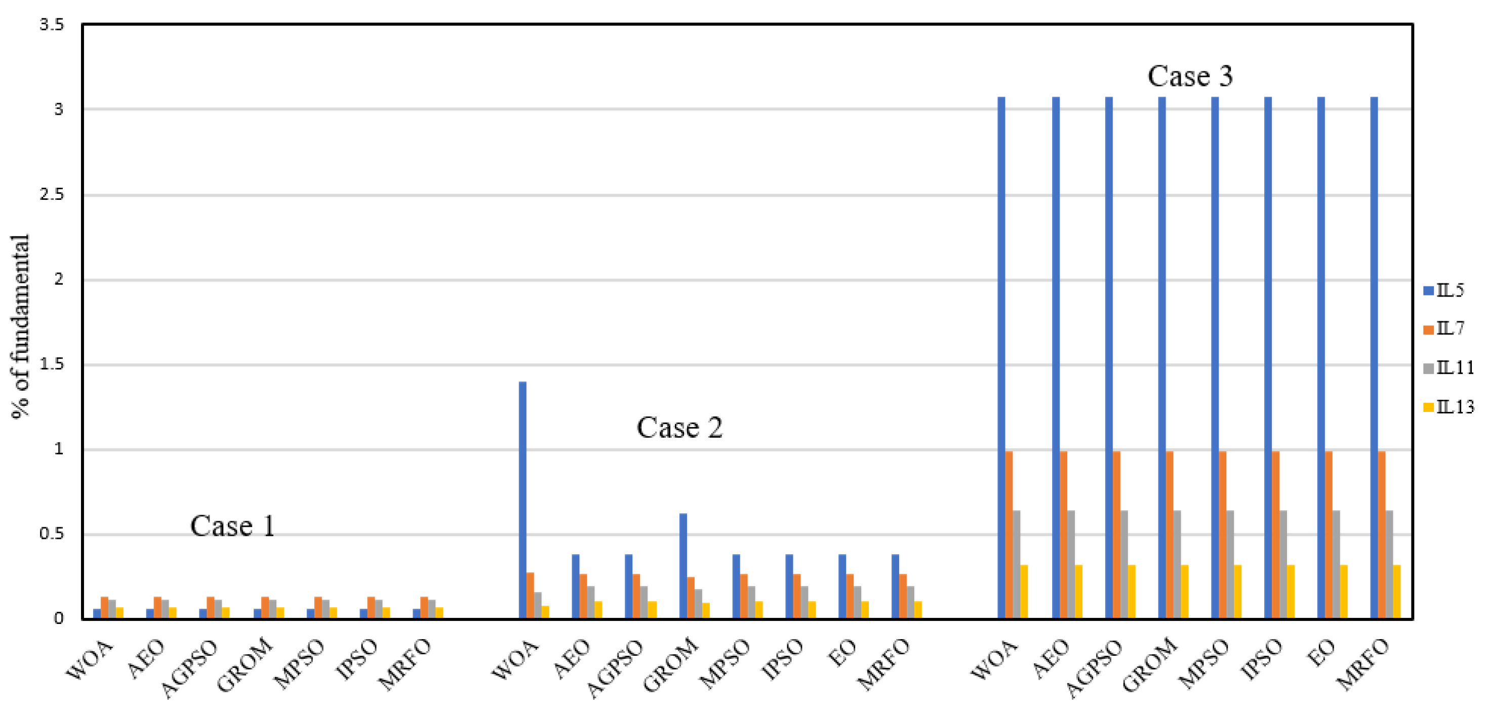
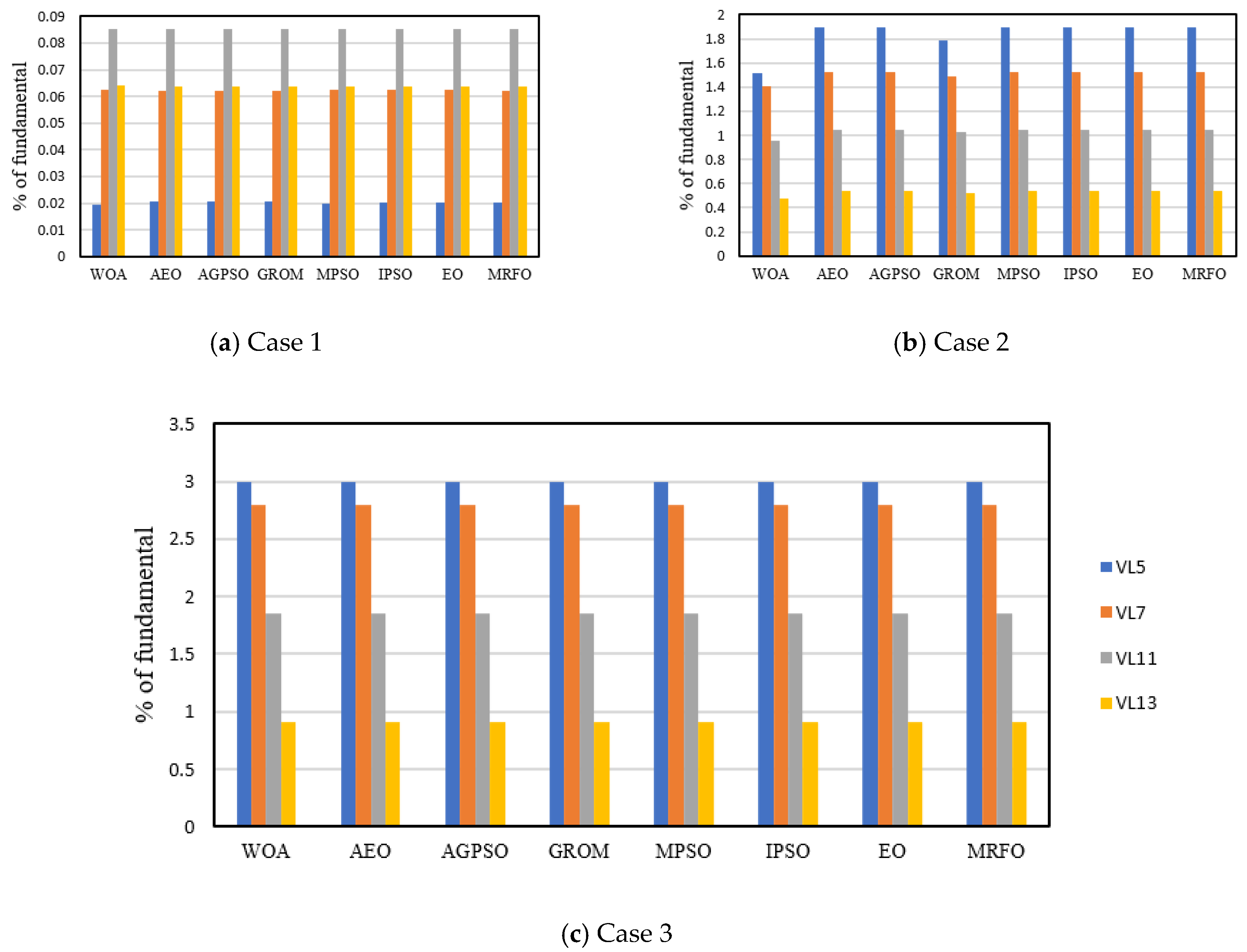
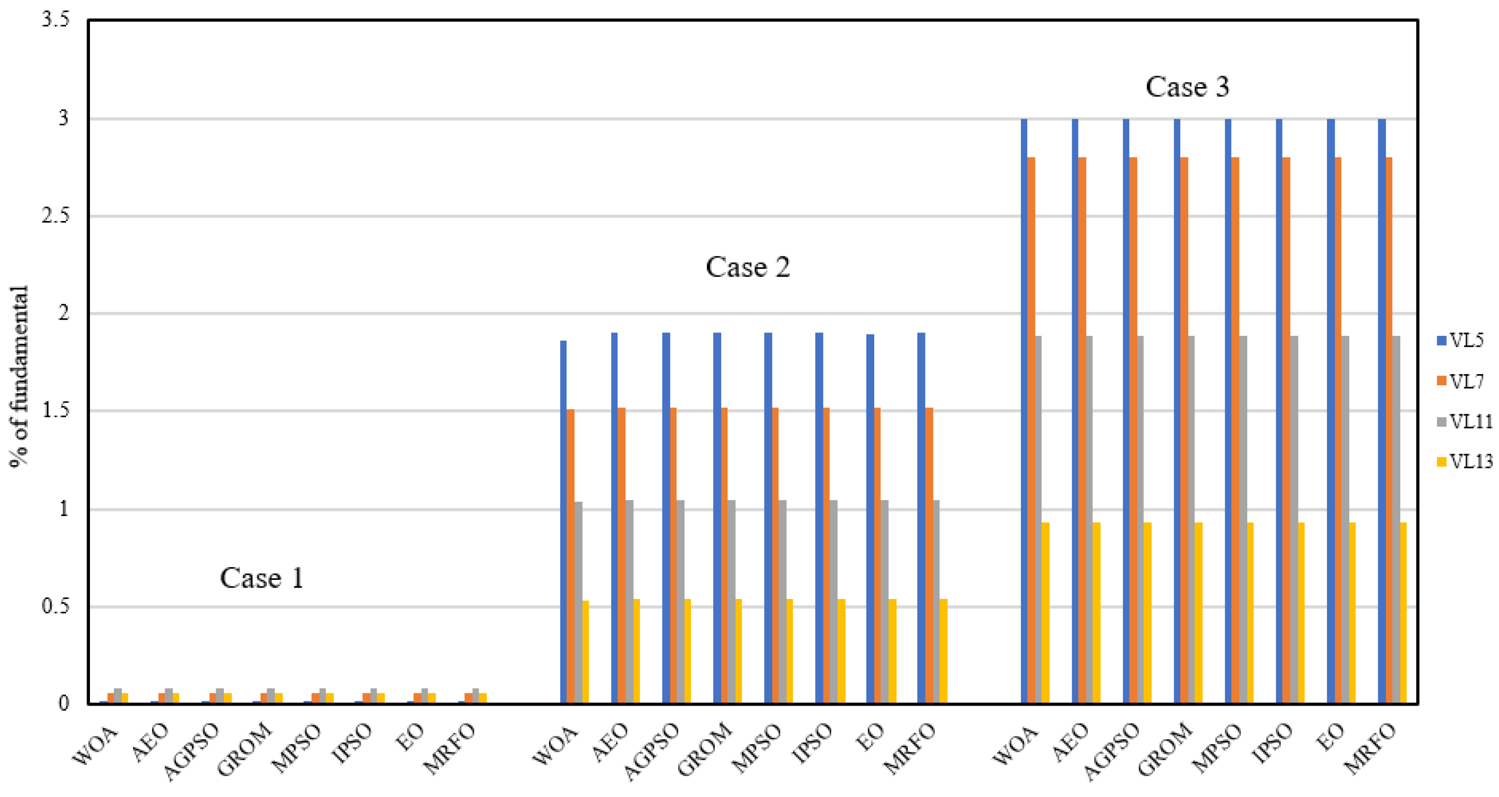
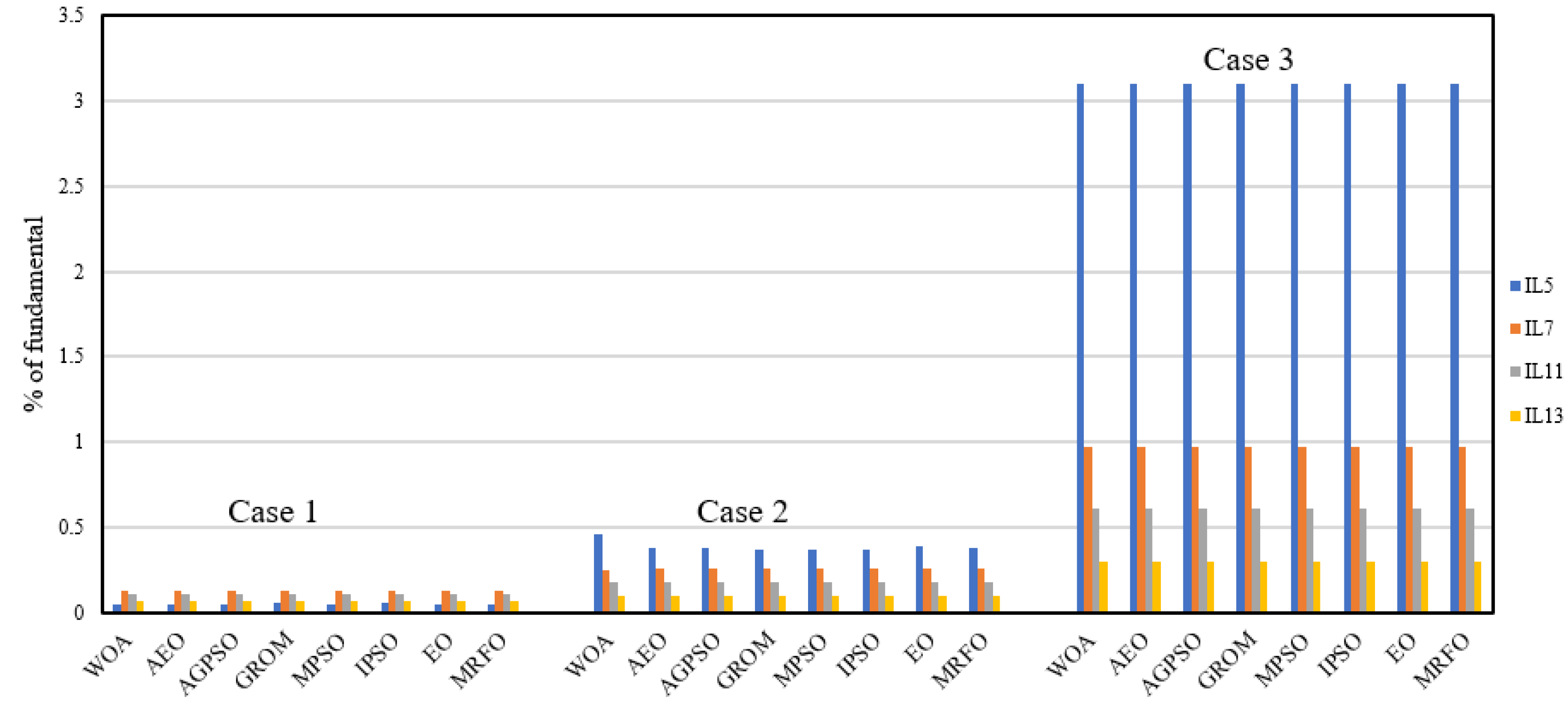
5.1. Harmonics Analysis under all Case STUDY Conditions

This section presents the performance of the optimization methods in this paper under different operation scenarios. Table 4 and Table 5 present the results of the proposed optimization algorithms for configurations 1 and 2 of HAPF over three different cases, as discussed in Section 4. The results in Table 4 and Table 5 show that the WOA outperformed all algorithms in terms of the HP for all cases. In addition, the proposed optimization method achieved a lower HP compared to L-SHADE [8] from the literature for all cases. In general, the results in Table 4 and Table 5 show that the increasing trend of voltage leads to an increase in the VTHD, ITHD and HP.

5.2. Results of Harmonics with Compensated System

Figure 4 and Figure 5 present the individual voltage and current harmonics ( V LH ) and ( I LH ), respectively, for various cases under HAPF configuration 1. The results presented in Figure 4 and Figure 5 show evidence that all optimization algorithms satisfied the achievement of limitation of harmonics required in standard IEEE 519, ( V LH 3 ) , I LH H = 5 , 7 < 4 , and   I LH H = 11 , 13 < 2 [8,20]. In Figure 4, the WOA outperformed the other proposed optimization algorithms by reducing the voltage harmonic ( V LH ). For example, the WOA reduced the voltage harmonic ( V L 5 ) at case 2 by 23% compared to other algorithms. The voltage and current harmonics ( V LH ) and ( I LH ) increased over the three cases with increasing voltage source harmonics. The WOA outperformed all algorithms and slightly improved the performance, except for the I L 5 in case 2, where the WOA recorded the highest value with 1.35%. However, the WOA for the I L 5 at case 2 satisfied the limitation ( I LH H = 5 , 7 < 4 ) .
The individual voltage and current harmonics, ( V LH ) and ( I LH ), for configuration 2 of HAPF are shown in Figure 6 and Figure 7, respectively. The results show that all optimization algorithms satisfied the limitation of harmonics. In addition, the results in this section showed that the increasing trend of voltage from cases 1 to 3 led to an increase in the harmonic level. In Figure 6 and Figure 7, the WOA outperformed the other proposed optimization algorithms by reducing the current harmonics ( I LH ). For example, the WOA in Figure 6 reduced the current harmonics ( I L 5 ) at cases 1 and 2 by 75%, and 5% compared to other algorithms. Similar to configuration 1, the voltage and current harmonics ( V LH ) and ( I LH ) increased over the three cases with increasing voltage source harmonics. The WOA outperformed all algorithms and slightly improved performance, except for the I L 5 in case 2, where the WOA recorded the highest value with 0.45%. However, the WOA for the I L 5 in case 2 satisfied the limitation ( I LH H = 5 , 7 < 4 ) . The results of all algorithms at configuration 2 showed better results compared to configuration 1.
Overall, the HAPF optimization problem is a complex and challenging task, which requires a balance between exploration and exploitation to avoid local optimal points and to achieve a global one. The results showed that the WOA algorithm is a very competitive algorithm, and was the best algorithm in almost all the cases, achieving a good balance between the exploration and exploitation phases. The WOA’s ability to derive the adaptive strategy and update the information helped in avoiding the extra number of iterations and achieved the optimal solution.

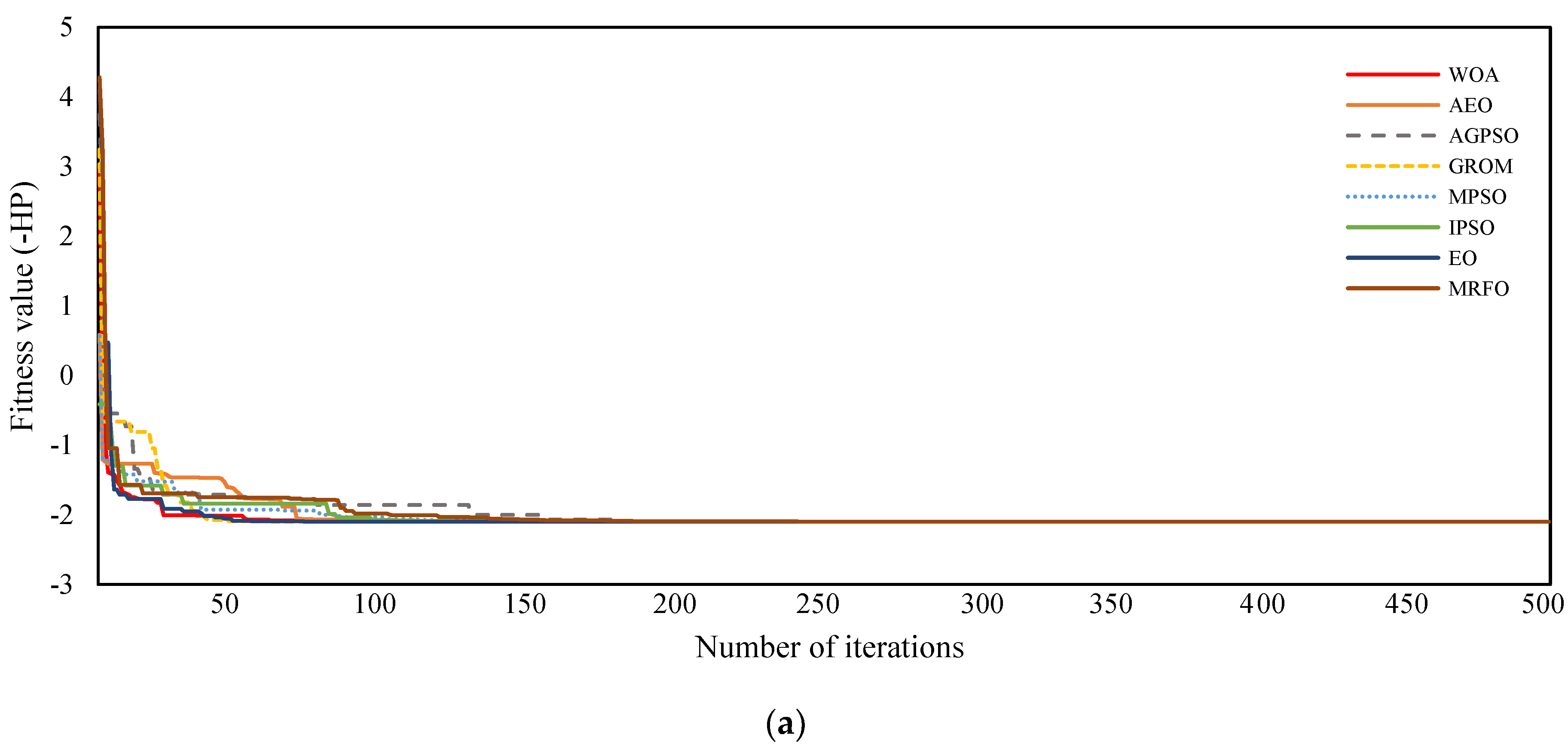
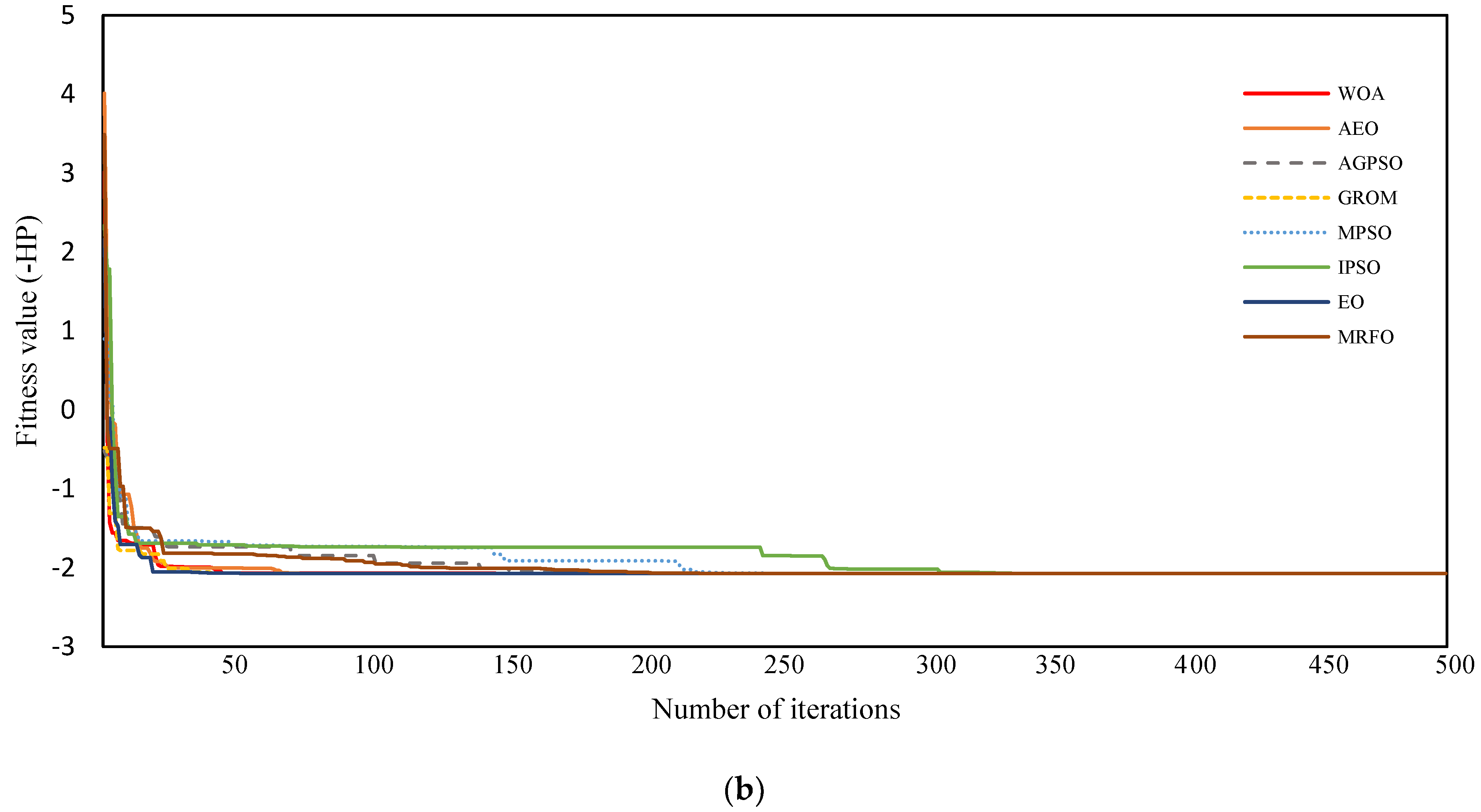
5.3. Comparative Performance and Statistical Analysis

To evaluate the convergence for the proposed optimization algorithms, convergence curves for all cases were generated over 500 iterations. The convergence curves show the relationship between the number of iterations and the HP value. The convergence curves introduce the speed of the optimization algorithm in achieving the final (optimal) solution. For example, Figure 8 shows the convergence results for all optimization algorithms for configurations 1 and 2 of the HAPF system within case 3 parameters. The results presented smooth convergence curves for all optimization algorithms. However, the WOA algorithm achieved the optimal solution with a smaller number of iterations compared to other algorithms. In addition, the GROM, AEO and EO algorithms showed similar convergence behavior to WOA. All algorithms achieved the optimal solution with less than 300 iterations for all cases, compared to the L-SHADE algorithm [8], which required more than 1500 iterations to achieve the optimal solution. The results in Figure 7 show that the proposed optimization algorithms in this paper are more efficient and powerful compared to L-SHADE [8], in terms of computational cost and higher efficiency in CPU utilization. In addition, the results of all algorithms at configuration 2 showed better results, in terms of the fitness value, by 10%, and in computational cost by 32%, compared to configuration 1. This is mainly due to the convergence curve of the WOA leaning towards being accelerated as iteration increases. The WOA convergence curve has been accelerated regarding the WOA searching for promising regions in the initial steps and can derive an adaptive strategy and update information to help to avoid an extra number of iterations.
In Section 1, the proposed optimization algorithms results were presented for all cases. This section provides further analysis of the performance of the optimization algorithms over 20 runs of simulations. The statistical analysis for all algorithms is presented in Table 6 considering the minimum, maximum, mean and standard deviation values of the HP value as a cost function. The WOA showed the most effective performance compared to other algorithms, achieving the lower value of the minimum values for all cases.

6. Conclusions

This work presented modern metaheuristic optimization algorithms for hybrid active power filters (HAPF). The proposed algorithms were employed to achieve the minimum HP by finding the optimal parameter design of HAPF under the limitations of harmonic distortion levels, as presented in the common standard IEEE 519. In addition, the robustness of the proposed algorithms was evaluated through two configurations of HAPF and in different case studies. The proposed optimization algorithm, WOA, was employed to improve the performance of HAPF compared to modern optimization algorithms (MRFO, AEO, GROM), and the common powerful optimization methods from literature (AGPSO, MPSO, IPSO, EO, L-SHADE). The WOA outperformed the other metaheuristic optimization algorithms and L-SHADE from the literature. The WOA outperformed the other proposed optimization algorithms, by reducing the current and voltage harmonics ( V LH , I LH ). For example, the WOA reduced the voltage harmonic ( V L 5 ) at case 2 by 23% and the I L 5   by 75% at case 1 (configuration 1), compared to other algorithms. The voltage and current harmonics ( V LH ) and ( I LH ) increased over the three cases with increasing voltage source harmonics. The results showed that the proposed modern optimization algorithms can improve power quality by successfully minimizing the VTHD, ITHD and HP to a lower level, compared to the literature. Hence, the investigation of the performance of the proposed modern metaheuristic optimization algorithms under various ranges of constraints, by using new techniques to handle the constraints, will be part of our future work.

Author Contributions

Conceptualization, F.A. and K.N.; methodology, K.N., F.A. and H.F.; software, K.N. and F.A.; validation, K.N. and F.A.; formal analysis, A.V., A.A., W.H. and F.A.; investigation, K.N. and F.A.; resources, all authors; data curation, all authors; writing—original draft preparation, F.A. and K.N.; writing—review and editing, all authors; visualization, all authors; supervision, all authors; project administration, F.A. and K.N. All authors have read and agreed to the published version of the manuscript.

Funding

This research received no external funding.

Acknowledgments

We would like to thank the Renewable Energy Center at The Hashemite University for their support.

Conflicts of Interest

The authors declare no conflict of interest.

Nomenclature

THDTotal Harmonic Distortions
HAPFHybrid Active Power Filters
PFPower Factor
HPHarmonic Pollution
WOAWhale Optimization Algorithm
MRFOManta ray foraging optimization
AEOArtificial Ecosystem-based Optimization
GROMGolden Ratio Optimization Method
PPFPassive Power Filter
APFActive Power Filter
PWMPulse Width Modulated
PSOParticle Swarm Optimization
DEDifferential Evolution
AGPSOAutonomous Groups Particles Swarm Optimization
MPSOModified Particle Swarm Optimization
IPSOImproved Particle Swarm Optimization
EOEquilibrium Optimizer
PCCPoint of common coupling
Z L inductive
Z C reactance
HAt harmonic H
V SH Voltage source
I SH current source
R SH transmission line resistance
L SH transmission line reactance
I LH load current
VTHDvoltage THD
ITHDvoltage THD
VTHD lim VTHD limitation
ITHD lim ITHD limitation
PF target target power factor

References

  1. Alasali, F.; Nusair, K.; Obeidat, A.M.; Foudeh, H.; Holderbaum, W. An analysis of optimal power flow strategies for a power network incorporating stochastic renewable energy resources. Int. Trans. Electr. Energy Syst. 2021, 31, e13060. [Google Scholar] [CrossRef]
  2. Alloui, N.; Fetha, C. Optimal Design for Hybrid Active Power Filter Using Particle Swarm Optimization. Trans. Electr. Electron. Mater. 2017, 18, 129–135. [Google Scholar]
  3. Nusair, K.; Alasali, F.; Hayajneh, A.; Holderbaum, W. Optimal placement of FACTS devices and power-flow solutions for a power network system integrated with stochastic renewable energy resources using new metaheuristic optimization techniques. Int. J. Energy Res. 2021, 45, 18786–18809. [Google Scholar] [CrossRef]
  4. Alasali, F.; El-Naily, N.; Zarour, E.; Saad, S.M. Highly sensitive and fast microgrid protection using optimal coordination scheme and nonstandard tripping characteristics. Int. J. Electr. Power Energy Syst. 2021, 128, 106756. [Google Scholar] [CrossRef]
  5. Alghamdi, T.A.H.; Anayi, F.; Packianather, M. Optimal Design of Passive Power Filters Using the MRFO Algorithm and a Practical Harmonic Analysis Approach including Uncertainties in Distribution Networks. Energies 2022, 15, 2566. [Google Scholar] [CrossRef]
  6. Pantoli, L.; Leuzzi, G.; Deborgies, F.; Jankovic, P.; Vitulli, F. A Survey of MMIC Active Filters. Electronics 2021, 10, 1680. [Google Scholar] [CrossRef]
  7. He, Q.; Liu, L.; Qiu, M.; Luo, Q. A Step-by-Step Design for Low-Pass Input Filter of the Single-Stage Converter. Energies 2021, 14, 7901. [Google Scholar] [CrossRef]
  8. Biswas, P.P.; Suganthan, P.; Amaratunga, G.A. Minimizing harmonic distortion in power system with optimal design of hybrid active power filter using differential evolution. Appl. Soft Comput. 2017, 61, 486–496. [Google Scholar] [CrossRef]
  9. Zeineldin, H.; Zobaa, F. Particle Swarm Optimization of Passive Filters for Industrial Plants in Distribution Networks. Electr. Power Compon. Syst. 2011, 39, 1795–1808. [Google Scholar] [CrossRef]
  10. Chang, Y.; Chinyao, L. An ant direction hybrid differential evolution heuristic for the large-scale passive harmonic filters planning problem. Expert Syst. Appl. 2008, 35, 894–904. [Google Scholar] [CrossRef]
  11. Mirjalili, S.; Lewis, A. The Whale Optimization Algorithm. Adv. Eng. Softw. 2016, 95, 51–67. [Google Scholar] [CrossRef]
  12. Zhao, W.; Zhang, Z.; Wang, L. Manta ray foraging optimization: An effective bio-inspired optimizer for engineering applications. Eng. Appl. Artif. Intell. 2020, 87, 103300. [Google Scholar] [CrossRef]
  13. Zhao, W.; Wang, L.; Zhang, Z. Artificial ecosystem-based optimization: A novel nature-inspired meta-heuristic algorithm. Neural Comput. Appl. 2020, 32, 9383–9425. [Google Scholar] [CrossRef]
  14. Nusair, K.; Alasali, F. Optimal Power Flow Management System for a Power Network with Stochastic Renewable Energy Resources using Golden Ratio Optimization Method. Energies 2020, 13, 3671. [Google Scholar] [CrossRef]
  15. Nematollahi, A.F.; Rahiminejad, A.; Vahidi, B. A novel meta-heuristic optimization method based on golden ratio in nature. Soft Comput. 2019, 24, 1117–1151. [Google Scholar] [CrossRef]
  16. Mirjalili, S.; Lewis, A.; Sadiq, A.S. Autonomous Particles Groups for Particle Swarm Optimization. Arab. J. Sci. Eng. 2014, 39, 4683–4697. [Google Scholar] [CrossRef] [Green Version]
  17. Biswas, P.P.; Suganthan, P.; Mallipeddi, R.; Amaratunga, G.A. Optimal power flow solutions using differential evolution algorithm integrated with effective constraint handling techniques. Eng. Appl. Artif. Intell. 2018, 68, 81–100. [Google Scholar] [CrossRef]
  18. Taher, M.A.; Kamel, S.; Jurado, F.; Ebeed, M. Optimal power flow solution incorporating a simplified UPFC model using lightning attachment procedure optimization. Int. Trans. Electr. Energy Syst. 2019, 30, e12170. [Google Scholar] [CrossRef]
  19. Ling, Y.; Zhou, Y.; Luo, Q. Lévy Flight Trajectory-Based Whale Optimization Algorithm for Global Optimization. IEEE Access 2017, 5, 6168–6186. [Google Scholar] [CrossRef]
  20. Dao, T.-K.; Pan, T.-S.; Pan, J.-S. A multi-objective optimal mobile robot path planning based on whale optimization algorithm. In Proceedings of the 2016 IEEE 13th International Conference on Signal Processing (ICSP), Chengdu, China, 6–10 November 2016; pp. 337–342. [Google Scholar]
  21. Peng, F.; Hirofumi, A.; Akira, N. A new approach to harmonic compensation in power systems-a combined system of shunt passive and series active filters. IEEE Trans. Ind. Appl. 1990, 26, 983–990. [Google Scholar] [CrossRef]
  22. IEEE Std. 519-2014; IEEE Recommended Practices and Requirements for Harmonic Control in Electrical Power Systems. IEEE Std.: Piscataway, NJ, USA, 2014.
Figure 1. The basic configuration of HAPF.
Electronics 11 01453 g001
Figure 2. The main circuit of configurations 1 and 2 of HAPF.
Electronics 11 01453 g002aElectronics 11 01453 g002b
Figure 3. A flow chart of Whale Optimization Algorithm (WOA) for the HAPF problem.
Electronics 11 01453 g003
Figure 4. The individual voltage harmonics for configuration 1 of HAPF under the proposed three cases.
Electronics 11 01453 g004
Figure 5. The individual current harmonics for configuration 1 of HAPF under the proposed three cases.
Electronics 11 01453 g005
Figure 6. The individual voltage harmonics for configuration 2 of HAPF under the proposed three cases.
Electronics 11 01453 g006
Figure 7. The individual current harmonics for configuration 2 of HAPF under the proposed three cases.
Electronics 11 01453 g007
Figure 8. The Convergence comparison results for all optimization algorithms for case study 3 (a) Configuration 1 of HAPF (b) Configuration 2 of HAPF.
Electronics 11 01453 g008aElectronics 11 01453 g008b
Table 1. The parameters of case studies for configuration 1 of HAPF.
ParametersCase 1Case 2Case 3
R S 1   ( Ω )0.021630.021630.02163
I S 1 (A)0.21630.21630.2163
R L 1   ( Ω )1.74211.74211.7421
Z L 1   ( Ω )1.6961.6961.696
V S 1 (KV)2.42.42.4
V S 5   ( % V S 1 )024
V S 7   ( % V S 1 )01.53
V S 11   ( % V S 1 )012
V S 13   ( % V S 1 )00.51
I L 5   ( % I L )404040
I L 7   ( % I L )666
I L 11   ( % I L )223
I L 13   ( % I L )112
Table 2. The parameters of case studies for configuration 2 of HAPF.
ParametersCase 1Case 2Case 3
R S 1   ( Ω )0.021630.021630.02163
I S 1 (A)0.21630.21630.2163
R L 1   ( Ω )1.74211.74211.7421
Z L 1   ( Ω )1.6961.6961.696
V S 1 (KV)2.42.42.4
V S 5   ( % V S 1 )024
V S 7   ( % V S 1 )01.53
V S 11   ( % V S 1 )012
V S 13   ( % V S 1 )00.51
I L 5   ( % I L )404040
I L 7   ( % I L )666
I L 11   ( % I L )222
I L 13   ( % I L )111
Table 3. The main parameters of the optimization algorithms.
AlgorithmParametersValues
MRFOSize of population100
Maximum iteration number500
Shape constant1
EOConstant values for controlling exploration (a1)2
Constant values for controlling exploitation (a2)1
Number of search particles100
Maximum number of iterations500
Generation probability0.5
IPSOCoefficient of inertiaDecreasing from 0.9 to 0.4 (linearly)
Search agent number100
Maximum iteration number500
Coefficient of acceleration1 and 2
AGPSOCoefficient of inertiaDecreasing from 0.9 to 0.4 (linearly)
Number of search agents100
Maximum iteration number500
AEOInertia coefficient1 and 2
Size of population100
Maximum number of iterations500
GROMGolden ratio1.618
Number of search agents100
Maximum number of iterations500
MPSOCoefficient of inertiaDecreasing from 0.9 to 0.4 (linearly)
Search agent number100
Maximum iteration number500
Coefficient of acceleration1 and 2
WOANumber of search agents100
Maximum number of iterations500
Table 4. The results of optimization algorithms for configuration 1 of the HAPF system over the three different cases.
Optimization Algorithm Z C ( Ω ) Z L   ( Ω ) F ( Ω ) I S (A) V L H (V)Transmission Efficiency (%)Transmission Loss (W)ITHD (%)VTHD (%)HP (%)
Case 1
WOA2.7096680.10393419.9999753.85072430.0899.2986416912,292.130.1997430.1252550.235766692
AEO2.7094280.10369420753.85072430.0899.2986416912,292.130.1999490.125010.235811789
AGPSO2.7094430.10370920753.85072430.0899.2986416912,292.130.1999350.1250250.235807572
GROM2.7093940.1036620753.85072430.0899.2986416912,292.130.1999820.1249760.23582184
MPSO2.7095760.10384220753.85072430.0899.2986416912,292.130.1998160.125160.235778556
IPSO2.7095230.10378920753.85072430.0899.2986416912,292.130.1998620.1251060.23578841
EO2.7095150.1037820753.85072430.0899.2986416912,292.130.1998690.1250970.235790216
MRFO2.7094790.10374519.9999753.85072430.0899.2986416912,292.130.1999020.1250610.235798895
L-SHADE [8]2.70940.1036520752.92431.5999.2912,2900.20.1250.236
Case 2
WOA2.608059019.9999753.6122430.5699.2989987112,284.351.4385862.3291652.737615864
AEO2.6996850.09168220753.55152430.7999.2991214912,282.370.5110792.7039042.7517811
AGPSO2.6995630.0915619.9999753.55162430.7999.2991213112,282.380.5115912.7033982.751378991
GROM2.6743070.06668419.6643753.61142430.7599.2990251212,284.330.6991792.5988712.751278888
MPSO2.6995010.09149920753.55162430.7999.2991212212,282.380.5118482.7031442.751177609
IPSO2.6995110.09150920753.55162430.7999.2991212412,282.380.5118042.7031872.751211422
EO2.699330.09132919.9966753.55182430.7999.2991209712,282.380.5126532.7024392.75063412
MRFO2.6990310.0910319.9848753.55192430.7999.2991206612,282.390.5142422.7011952.749708921
L-SHADE [8]2.69980.0917620753.552430.899.312,2800.5112.7042.752
Case 3
WOA2.61587709.75041752.89642431.8699.3000313112,261.033.3076984.5945555.661343106
AEO2.615877 4.85 × 10 17 9.75103752.89642431.8699.3000313412,261.033.3074914.5946065.661263412
AGPSO2.61587709.75103752.89642431.8699.3000313412,261.033.3074914.5946065.661263412
GROM2.61587709.75103752.89642431.8699.3000313412,261.033.3074914.5946065.661263412
MPSO2.61587709.75103752.89642431.8699.3000313412,261.033.3074914.5946065.661263412
IPSO2.61587709.75103752.89642431.8699.3000313412,261.033.3074914.5946065.661263412
EO2.61587709.75103752.89642431.8699.3000313412,261.033.3074914.5946065.661263412
MRFO2.615877 1.25   ×   10 7 9.75101752.89642431.8699.3000313312,261.033.3074934.5946065.66126432
L-SHADE [8]2.6159 1.36   ×   10 8 9.75752.92431.8799.312,2603.3064.6095.672
Table 5. The results of optimization algorithms for configuration 2 of HAPF system over the three different cases.
Optimization Algorithm Z C ( Ω ) Z L ( Ω ) F ( Ω ) I S   ( A ) V L H   ( V ) Transmission Efficiency (%)Transmission Loss (W)ITHD (%)VTHD (%)HP (%)
Case 1
WOA2.7105050.1047723020753.85072430.0899.2986416212,292.132980.1924390.121026360.22730
AEO2.7101150.1043824420753.85072430.0899.2986416212,292.13310.1926570.120642630.22731
AGPSO12.7100180.1042855120753.85072430.0899.2986416212,292.133130.1927310.120551030.22732
GROM2.7099040.1041712919.9999753.85072430.0899.2986416112,292.133150.1928290.120445090.22735
MPSO2.7099840.1042519420753.85072430.0899.2986416212,292.133130.1927590.120519670.22733
IPSO2.7099420.1042097220753.85072430.0899.2986416112,292.133140.1927950.120480480.22734
EO2.7099790.1042467820753.85072430.0899.2986416212,292.133130.1927630.120514860.22733
MRFO2.7100620.1043297819.9999753.85072430.0899.2986415912,292.133660.1926960.120592950.22732
L-SHADE [8]2.70990.1041620753.852430.0999.2912,2900.1930.120.2274
Case 2
WOA2.6908020.0828436420753.55932430.7799.2991079212,282.632640.5593112.665089952.72314
AEO2.7005160.0925142519.9999753.55132430.7999.2991218412,282.370630.5036532.705120082.75160
AGPSO2.7006480.0926452420753.55112430.7999.2991220812,282.365930.5030842.705660052.75203
GROM2.7012440.0932384220753.55062430.7999.2991229712,282.348780.5005712.708104752.75397
MPSO2.7011800.0931746420753.55072430.7999.2991228512,282.351210.5008362.707841972.75376
IPSO2.7011080.0931033120753.55072430.7999.2991227412,282.35320.5011342.707548032.75353
EO2.6990220.0910276619.9998753.55252430.7999.2991197312,282.41070.5104922.698987202.74684
MRFO2.7008270.0927929419.9993753.54682430.7999.2991287112,282.224030.5024732.706266882.75251
L-SHADE [8]2.70130.0933120753.552430.899.312,28000.52.7082.754
Case 3
WOA2.616002 5.096 × 10 5 10.3001752.88772431.8799.3000444212,260.746873.3123694.615496775.680073
AEO2.615950 2.19   ×   10 16 10.3055752.88772431.8799.3000444212,260.747763.3118764.615497565.680787
AGPSO12.615950010.3055752.88772431.8799.3000444212,260.747763.3118764.615497565.680787
GROM2.615950 2.16   ×   10 16 10.3055752.88772431.8799.3000444212,260.747763.3118764.615497565.680787
MPSO2.615950010.3055752.88772431.8799.3000444212,260.747763.3118764.615497565.680787
IPSO2.615950010.3055752.88772431.8799.3000444212,260.747763.3118764.615497565.680787
EO2.615950010.3055752.88772431.8799.3000444212,260.747763.3118764.615497565.680787
MRFO2.615950 1.119   ×   10 7 10.3055752.88772431.8799.3000444112,260.748113.3118774.615497565.680787
L-SHADE [8]2.6188 1.81   ×   10 4 8.84752.682431.8899.312.263.3124.6155.6814
Table 6. The statistical analysis results of all optimization algorithms for the different HAPF systems.
Case Study of HAPFOptimization AlgorithmMinimumMaximumMeanStandard
Deviation
Configuration 1/Case1WOA0.2357666920.4698260.2376650.052876309
AEO0.2358117890.2358260.235824 3.04936   ×   10 6
AGPSO0.2358075720.2359160.235825 2.51373   ×   10 5
GROM0.235821840.4929870.2358250.057503316
MPSO0.2357785560.4929870.235830.1055344
IPSO0.235788410.4929790.2358210.05750202
EO0.2357902160.2366370.2358240.000185485
MRFO0.2357988950.2358670.235827 1.46314   ×   10 5
Configuration 1/Case2WOA2.7376158642.817522.7569030.018962596
AEO2.75178112.9525272.7520290.084461027
AGPSO2.7513789912.7522782.7519710.000253608
GROM2.7512788882.9524262.7520290.047503307
MPSO2.7511776092.752862.7519550.000359295
IPSO2.7512114222.7531542.752050.000505761
EO2.750634122.7533592.752020.000497049
MRFO2.7497089212.9524462.7523140.082200423
Configuration 1/Case3WOA5.6010296786.0758895.6680140.141450192
AEO5.6612634125.8749275.6612630.087682408
AGPSO5.6612634125.8749275.6612630.103770037
GROM5.6612634125.6612645.661263 4.46357   ×   10 8
MPSO5.6612634125.874935.8749270.104558563
IPSO5.6612634125.8749275.8749270.107392539
EO5.6612634125.8749275.6612640.065595524
MRFO5.661264325.8749285.6613810.077773785
Configuration 2/Case1WOA0.2273333750.3743460.2288520.032383272
AEO0.2273134110.45880.2273580.071226658
AGPSO0.2273279580.2274060.227359 1.71045 × 10 5
GROM0.227355140.45880.2273580.051752048
MPSO0.2273348080.227390.227359 1.3785   ×   10 5
IPSO0.2273447480.4588070.2273680.113256767
EO0.2273359440.2277370.2273580.000113333
MRFO0.2273208640.2273780.227362 1.38645   ×   10 5
Configuration 2/Case 2WOA2.7231477382.7801972.75490.015270307
AEO2.7516071552.9490882.7542180.04358177
AGPSO2.752033822.7545392.754160.000518827
GROM2.7539795312.7543412.754198 7.40857   ×   10 5
MPSO2.7537692822.754942.7541480.000265005
IPSO2.7535344242.9490482.7541540.043576249
EO2.7468407972.7570012.754190.002199937
MRFO2.7525188362.9491412.754310.059895568
Configuration 2/Case 3WOA5.6800738156.0818725.6870810.095893203
AEO5.6807870985.682095.6807870.000291242
AGPSO5.6807870985.9060815.9060810.114994201
GROM5.6807870985.8495215.6807870.037730048
MPSO5.6807870985.9060815.9060810.092458845
IPSO5.6807870985.9060815.9060810.110250146
EO5.6807870985.6915755.6807890.003574488
MRFO5.6807876745.681095.680795 8.22709   ×   10 5
Publisher’s Note: MDPI stays neutral with regard to jurisdictional claims in published maps and institutional affiliations.

