Convolutional Neural Network-Based Radar Antenna Scanning Period Recognition

Abstract

The antenna scanning period (ASP) of radar is a crucial parameter in electronic warfare (EW) which is used in many applications, such as radar work pattern recognition and emitter recognition. For antennas of radars and EW systems, which perform scanning circularly, the method based on threshold measurement is invalid. To overcome this shortcoming, this study proposes a method using the convolutional neural network (CNN) to recognize the ASP of radar under the condition that antennas of the radar and EW system both scan circularly. A system model is constructed, and factors affecting the received signal power are analyzed. A CNN model for rapid and accurate ASP radar classification is developed. A large number of received signal time–power images of three separate ASPs are used for the training and testing of the developed model under different experimental conditions. Numerical experiment results and performance comparison demonstrate high classification accuracy and effectiveness of the proposed method in the condition that antennas of radar and EW system are circular scan, where the average recognition accuracy for radar ASP is at least 90% when the signal to-noise ratio (SNR) is not less than 30 dB, which is significantly higher than the recognition accuracy of NAC and AFT methods based on adaptive threshold detection.

1. Introduction

With the development of integrated radio frequency systems, it has been common for radar and electronic warfare (EW) equipment to share the same antenna [1]. To cover the 360-degree airspace, a radar antenna often scans circularly [2]. When the EW system antenna scans circularly as well as the radar antenna, this is not beneficial to the EW system to estimate the antenna scanning period (ASP) of a hostile radar. In reality, radars can have different values of ASP, and different ASP values correspond to different operating modes [2]. Therefore, to achieve precise reconnaissance for specific radar, the EW system must determine the ASP values in real-time and accurately, which is helpful to deduce the composition of the enemy defense system and discover monitoring blind spots [3,4]. Moreover, it is useful to set parameters of a jammer [3]. A change in the ASP is also crucial in determining the threat levels of a radar [5]. Thus, it is significant that the EW system estimates radar ASP when an antenna scans circularly.

Generally, after sorting the intercepted pulse train, the ASP can be estimated according to the reference times of different received signals. Assume that the reference time of the ith pulse set is t_i, and the reference time of the jth pulse set is t_j, then the ASP of radar is calculated as $T=\left(t_j-t_i\right)/\left(j-i\right)$ [6,7]. There are three methods that use different pulses of the received radar signal to evaluate the reference time. The first method is to detect the rising edge of the first pulse in the received radar pulse set as a reference time [8,9]. The second method is to use the receipt time of the largest amplitude pulse in the received pulse set as a reference time [10]. In the third method, the average arrival time of all received pulses modulated by the main-beam pattern (MBP) of a radar antenna is regarded as a reference time [11]. These methods have the advantages of being simple and easy to understand, but their disadvantages are also obvious. In fact, the reference time is not easy to determine because of the noise influence, so the ASP of radar cannot be determined accurately. Barshan and Eravci et al. [6,7] introduced an ASP estimation algorithm based on the normalized autocorrelation coefficient (NAC) of a signal sample sequence, which can detect the main beam in the pulse sets by finding its maximum peak value using the two index points on each side of the maximum peak point. Wan et al. [9] reconstructed the MBP curve of a radar antenna based on the received multiple periodic radar pulse signals and then estimated the ASP of the radar according to time difference in the obtained MBP curves. In essence, the above-mentioned methods are based on the fact that the arrival time interval of the maximum signal amplitude is equal to the ASP, so the ASP is obtained by estimating the time difference in the maximum peak value based on the adaptive threshold. These methods are effective in the case that an antenna of the EW system is stationary without rotating. However, when the EW system’s antenna scans circularly, the power of the signal received by the EW system is not determined only by radar antenna rotating but also by the EW system antenna rotating, so the arrival time interval of the maximum signal amplitude is not necessarily equal to the radar ASP. The existing methods suffer from the ambiguity problem in the radar ASP estimation when the NAC and MBP are used [10]. When antennas of the EW system scan circularly, there has been no relevant solution to the problem of how to estimate radar ASP. Therefore, the estimation of radar ASP, under the condition that the antennas of the radar and EW system scan circularly, is worth studying.

The convolutional neural network (CNN) is a variant of a feed-forward neural network, and it is a powerful model for solving classification problems. Lecun et al. [11] applied CNN to handwritten digit recognition and achieved good results. Deep learning based on CNN has become the focus in the classification field, and many advanced networks have been designed using CNNs, such as AlexNet [12], ResNet [13], and GoogLeNet [14]. Since the impressive classification accuracy of CNN, many researchers tried to apply it to radar and EW field. CNN was applied to automatically recognize radar waveform using the radar signal time-frequency images as the input of network [15]. Lindsay Cain investigated an application of CNN for rapid and accurate classification of EW emitters [16]. Aleksandar Angelov used different CNNs and automotive radar data to classify the class of targets (car, single and multiple people, bicycle) [17]. Ahmet M.Elbir constructed a CNN as a multi-class classification framework to make a cognitive antenna selection [18]. Hidetoshi Furukawa dealy with translation invariance of convolutional neural networks for automatic target recognition from synthetic aperture radar (SAR) imagery [19]. In this paper, we apply the idea of deep learning to classify the ASP of hostile radar followed prior information. Owing to the high classification accuracy of CNN, this study applies CNN to classify the radar ASP.

This work has been inspired by the work of Kim et al. [20,21], and a system model for the case when the transmitting and receiving antennas scan circularly is developed. The signal received by the EW system is transformed into time–power images, and a CNN is designed to classify the ASP using the labeled training dataset. This work assumes the number of ASP that needs to be classified is small and the processing speed is fast, so a simple and effective CNN is designed to solve the problem associated with the recognition of the radar antenna scanning period.

The rest of the study is organized as follows. Section 2 analyzes the problem background and constructs a system model for the case when, on the stationary platform, both radar and EW system antennas scan circularly, considering that dominant factors determine the received signal power of the EW system. Section 3 introduces the classification procedure of the radar ASP based on CNN and explains the architecture of the designed CNN model. Section 4 presents numerical experiments where the proposed CNN is trained and tested using the labeled training data generated by simulations. The experimental results and analysis are given and discussed in Section 5. Finally, Section 6 concludes the paper.

2. System Model and Problem Analysis

2.1. System Model

Circular scanning has been widely used for surveillance radars. The radar antenna scans a range of 360° in the azimuth at a constant rate, while the elevation angle is kept fixed. This work considers that antennas of both the radar and the EW system scan circularly.

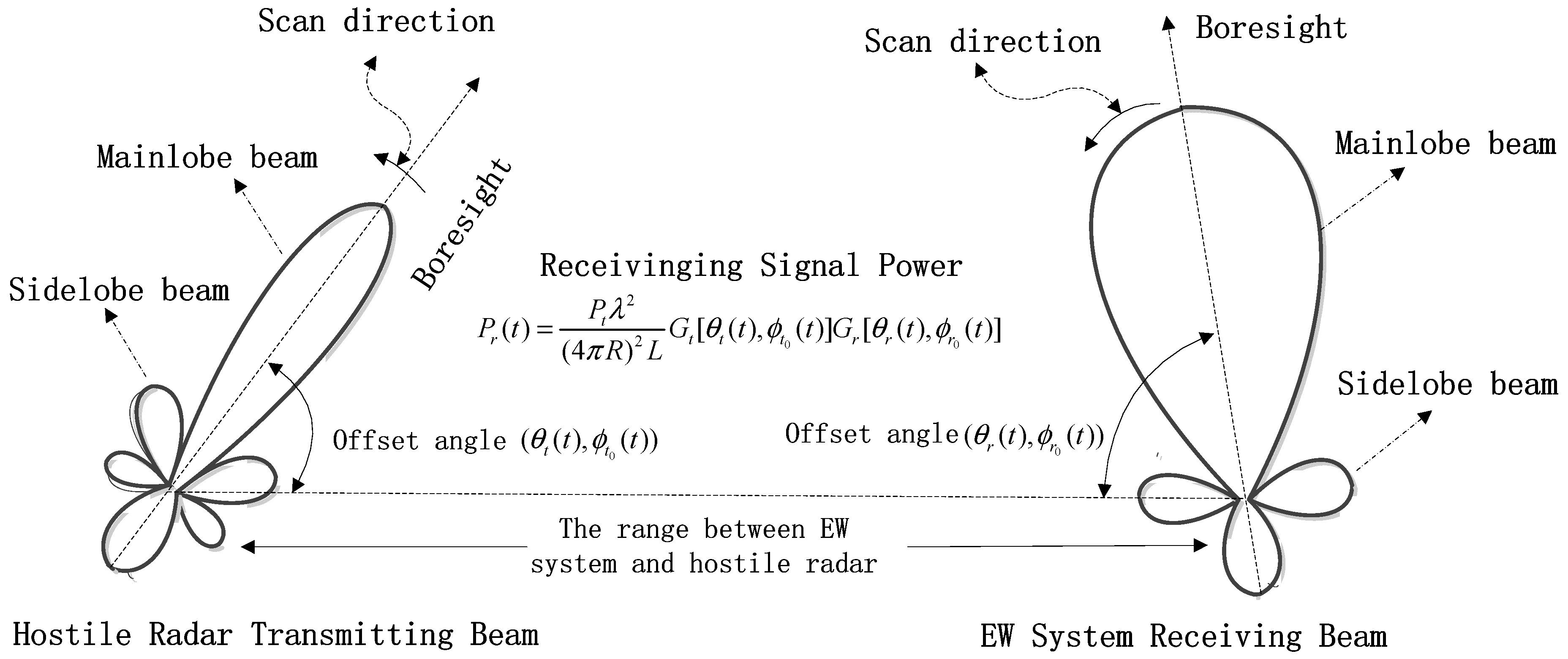
First, the model of the received signal power in an EW system is constructed under the assumption that antennas of the radar and EW system mounted on a stationary platform scan circularly. Generally, the radar transmitting antenna has a narrow beam used to increase the spatial resolution and to extend the detection range, so most of the transmitting power is concentrated in the boresight direction, i.e., in the main lobe beam direction. Since the boresight direction of an antenna is a direction in which the antenna gain is maximum, the received signal of the EW system has the maximum power when the boresight of a radar antenna passes through the boresight of the EW system antenna. When the distance between an EW system and a radar is R, the received signal power $P_r$ is calculated as

$$P_r\left(t\right)=\frac{P_t{\lambda }^2}{{\left(4\mathsf{\pi }R\right)}^{2}L}{G}_t\left[{\theta }_t\left(t\right),{\varphi }_t\left(t\right)\right]G_r\left[{\theta }_r\left(t\right),{\varphi }_r\left(t\right)\right],$$

(1)

where $P_t$ and $\lambda$ denote the radar transmitting power and signal wavelength, respectively; $L$ denotes the system loss factor, including atmospheric propagation loss and polarization mismatch loss between radar antenna and EW system antenna; ${\theta }_t\left(t\right)$ and ${\theta }_r\left(t\right)$ denote the azimuth angles of the transmitting antenna and receiving antenna, respectively; ${\varphi }_t\left(t\right)$ and ${\varphi }_r\left(t\right)$ denote the elevation angles of the transmitting antenna and receiving antenna, respectively; $\left({\theta }_t\left(t\right),{\varphi }_t\left(t\right)\right)$ is the radar antenna boresight offset angle in the EW system direction at time $t$; (${\theta }_r\left(t\right),{\varphi }_r\left(t\right)$) is the EW system boresight offset angle in the radar direction at time $t$; $G_t\left[{\theta }_t\left(t\right),{\varphi }_t\left(t\right)\right]$ is the radar transmitting antenna gain in the EW system direction at time $t$; $G_r\left[{\theta }_r\left(t\right),{\varphi }_r\left(t\right)\right]$ is the EW system antenna gain in the radar direction at time $t$. Commonly, the radar transmitting power $P_t$ is constant, so term $P_t{\lambda }^2/{\left(4\mathsf{\pi }R\right)}^2$ in Equation (1) is assumed to be constant because the range between radar and EW system is considered changing negligibly. The loss factor $L$ is estimated as a constant. Therefore, there are two dominant factors determining the received signal power under the condition that radar and EW system’ antennas scan circularly, namely, $G_t\left[{\theta }_t\left(t\right),{\varphi }_t\left(t\right)\right]$ and $G_r\left[{\theta }_r\left(t\right),{\varphi }_r\left(t\right)\right]$. As the radar and EW system antennas rotate, $G_t\left[{\theta }_t\left(t\right),{\varphi }_t\left(t\right)\right]$ and $G_r\left[{\theta }_r\left(t\right),{\varphi }_r\left(t\right)\right]$ vary with time $t$, and are respectively calculated as

$$G_t\left[{\theta }_t\left(t\right),{\varphi }_t\left(t\right)\right]=G_T{F}_t\left[{\theta }_t\left(t\right),{\varphi }_t\left(t\right)\right],$$

(2)

$$G_r\left[{\theta }_r\left(t\right),{\varphi }_r\left(t\right)\right]=G_R{F}_r\left[{\theta }_r\left(t\right),{\varphi }_r\left(t\right)\right],$$

(3)

where $G_T$ and $F_t\left[{\theta }_t\left(t\right),{\varphi }_t\left(t\right)\right]$ denote the maximum gain and normalized beam pattern of an antenna, respectively; $G_R$ and $F_r\left[{\theta }_r\left(t\right),{\varphi }_r\left(t\right)\right]$ denote the maximum gain and normalized beam pattern of an EW system antenna.

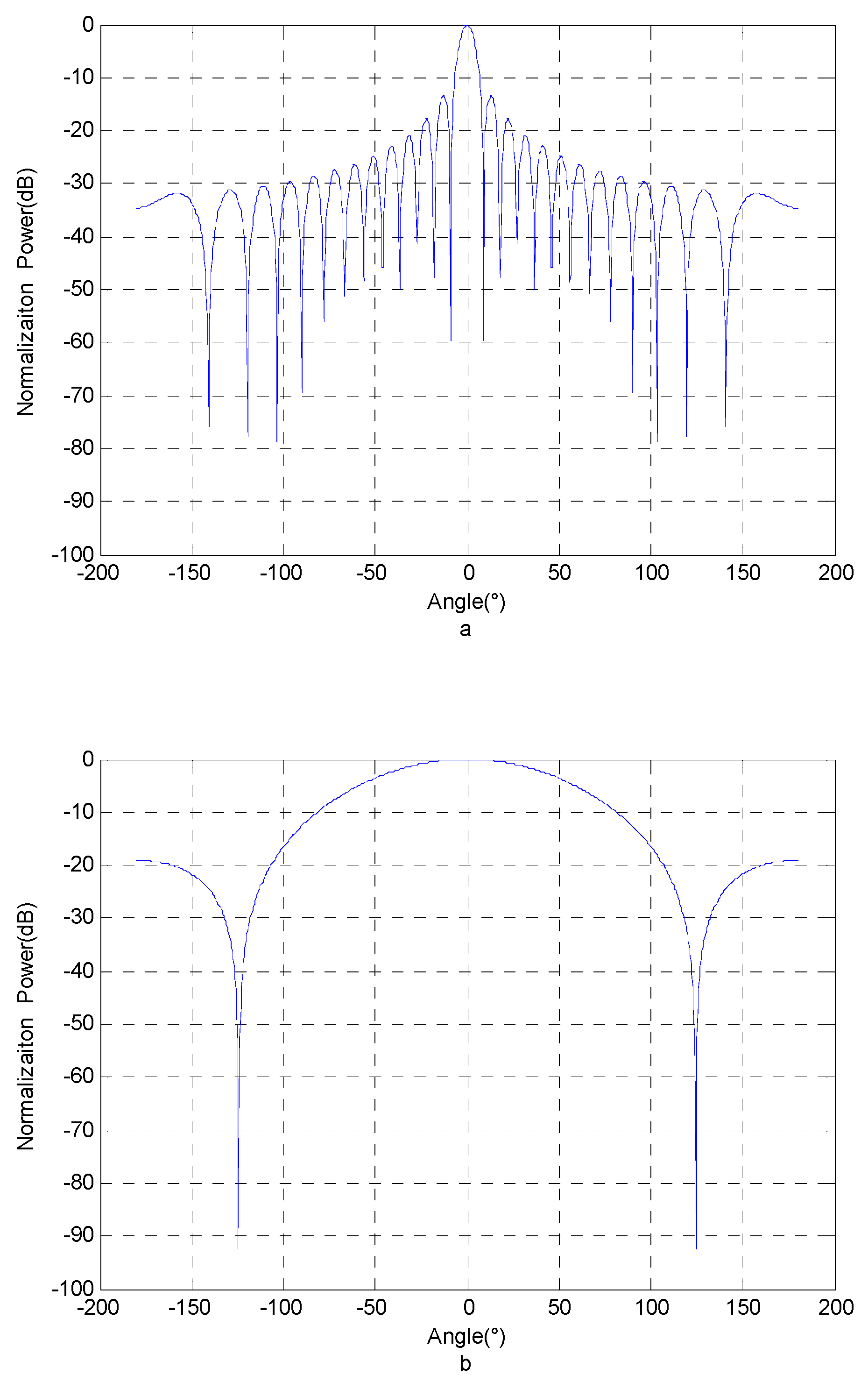
The antenna beam pattern $F\left[\theta ,\varphi \right]$ is defined by the antenna aperture shape and illumination function. However, since beam patterns do not have closed-form expressions, this paper considers only the beam pattern of a uniformly illuminated rectangular aperture radar, and its closed-form expression is given by [22]:

$$F\left[\theta ,\varphi \right]={\left[\frac{\sin \left(k_1\sin \frac{\theta }{k_3}\cos \frac{\varphi }{k_3}\right) \sin \left(k_2\sin \frac{\varphi }{k_3}\cos \frac{\theta }{k_3}\right)}{\left(k_1\sin \frac{\theta }{k_3}\cos \frac{\varphi }{k_3}\right) \left(k_2\sin \frac{\varphi }{k_3}\cos \frac{\theta }{k_3}\right)}\right]}^2,$$

(4)

where the shape and beamwidth of the main lobe can be modified by adjusting coefficients $k_1$ and $k_2$. The sidelobe number and antenna beam directivity can be changed by tuning $k_3$. The antenna gain is calculated by [15]:

$$G\approx 10 {\log }_{10}\left(\frac{26000}{{\theta }_B{\varphi }_B}\right),$$

(5)

where ${\theta }_B$ and ${\varphi }_B$ are the 3-dB azimuth beamwidth and 3-dB elevation beamwidth of an antenna, and they are defined by $F\left[\theta ,\varphi \right]$. Therefore, once the beam patterns of the radar and EW system’s antennas are designed, the gains of the radar and EW system are fixed, and $F\left[\theta ,\varphi \right]$ value is defined by the antenna boresight offset angle. If the EW system antenna is stationary without rotating, the azimuth and elevation angles are unchanging; hence, (${\theta }_r\left(t\right),{\varphi }_r\left(t\right)$) is constant over time, and the received signal power of the EW system varies only with $({\theta }_t\left(t\right),{\varphi }_t\left(t\right))$. However, when the radar and EW system’s antennas rotate, the received signal power of the EW system varies with both $({\theta }_t\left(t\right),{\varphi }_t\left(t\right))$ and $({\theta }_r\left(t\right),{\varphi }_r\left(t\right))$. When antennas of the radar and EW system scan circularly, as depicted in Figure 1, the azimuth angles ${\theta }_t\left(t\right)$ and ${\theta }_r\left(t\right)$ vary with antenna rotation, but the elevation angles ${\varphi }_t\left(t\right)$ and ${\varphi }_r\left(t\right)$ are constant; thus, $G_t\left[{\theta }_t\left(t\right),{\varphi }_t\left(t\right)\right]$ and $G_r\left[{\theta }_r\left(t\right),{\varphi }_r\left(t\right)\right]$ vary only with azimuth angles at time t. Accordingly, the radar’s transmitting antenna gain in the EW system direction and the EW system’s receiving antenna gain in the radar direction are denoted by $G_t\left[{\theta }_t\left(t\right),{\varphi }_{t_0}\left(t\right)\right]$ and $G_r\left[{\theta }_r\left(t\right),{\varphi }_{r_0}\left(t\right)\right]$, respectively, and ${\varphi }_{t_0}\left(t\right)$ and ${\varphi }_{r_0}\left(t\right)$ 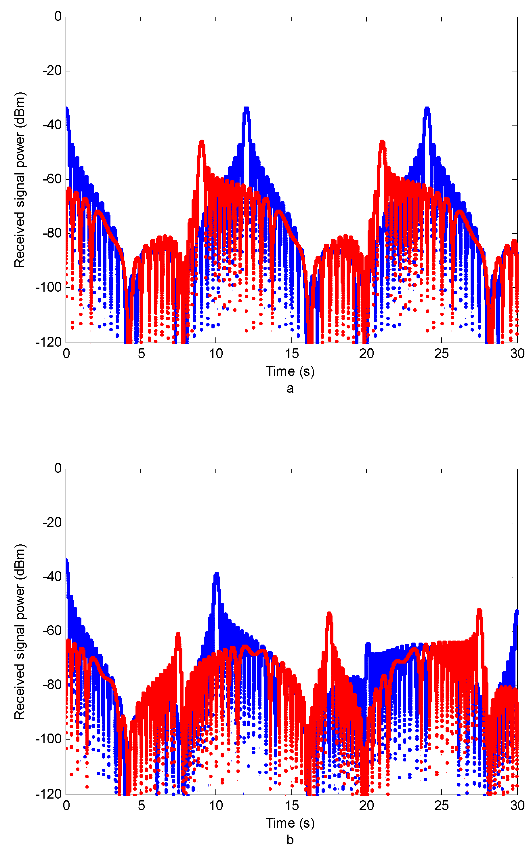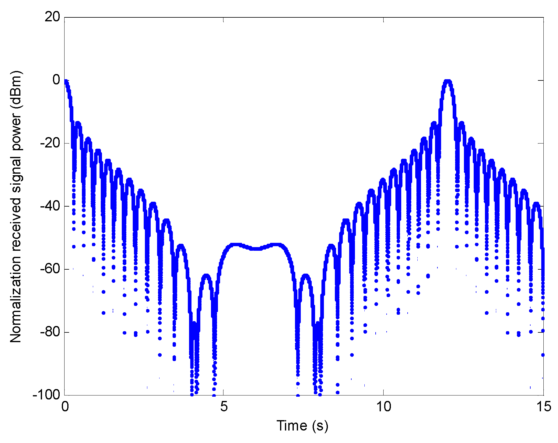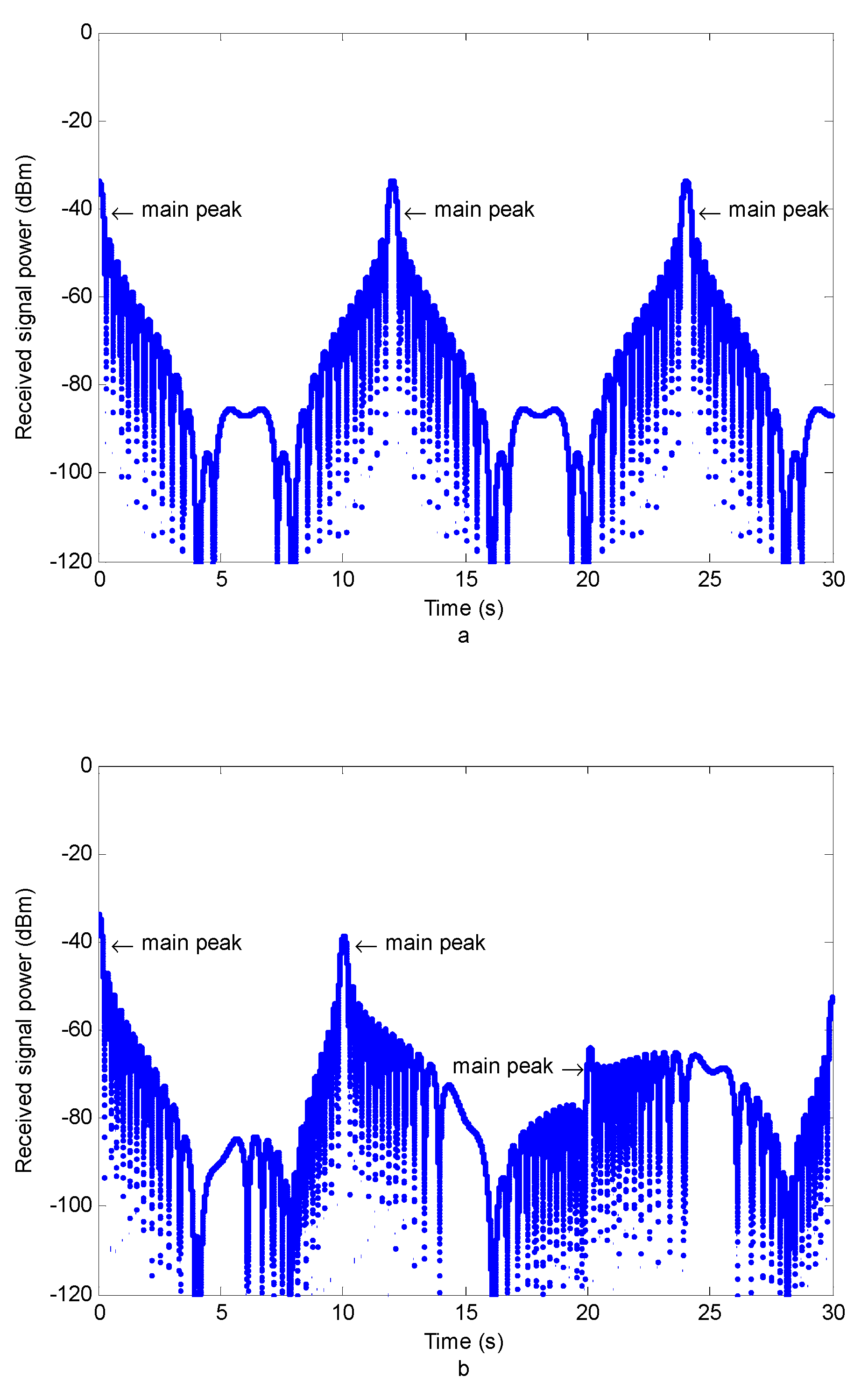are constant. Circular scanning defines the transmitting and receiving beam boresight offset angles. When the radar’s transmitting beam boresight faces directly to the EW system, and EW system’s receiving beam boresight faces directly to the radar, the radar antenna’s main lobe beam covers the EW system, and the EW system antenna’s main lobe beam covers the radar at the same time. Hence, the product of $G_t\left[{\theta }_t\left(t\right),{\varphi }_{t_0}\left(t\right)\right]$ and $G_r\left[{\theta }_r\left(t\right),{\varphi }_{r_0}\left(t\right)\right]$ is maximum, which causes a main peak in the received signal time–power images. When the product of $G_t\left[{\theta }_t\left(t\right),{\varphi }_{t_0}\left(t\right)\right]$ and $G_r\left[{\theta }_r\left(t\right),{\varphi }_{r_0}\left(t\right)\right]$ is minimum at time $t$, the received signal of the EW system has the minimum power, which causes a valley value.

2.2. Problem Analysis

The beam pattern of a transmitting antenna and a receiving antenna are defined by Equation (4). Suppose that a radar antenna is an array antenna with circular scanning and a narrow main lobe. Assume $k_1=40$, $k_2=3$, $k_3$ = 2, $\varphi =0.01$, ${\theta }_t=\left[-\mathsf{\pi }:\mathsf{\pi }/360:\mathsf{\pi }\right]$, and ${\varphi }_t=0.01$, then,

$$F\left[{\theta }_t,{\varphi }_t\right]={\left[\frac{\sin \left(40\sin \frac{{\theta }_t}{2}\cos \frac{0.01}{2}\right) \sin \left(3\sin \frac{0.01}{2}\cos \frac{{\theta }_t}{2}\right)}{\left(40\sin \frac{{\theta }_t}{2}\cos \frac{0.01}{2}\right) \left(3\sin \frac{0.01}{2}\cos \frac{\theta }{2}\right)}\right]}^2.$$

(6)

The normalization beam pattern of a radar antenna is presented in Figure 2a. The 3-dB azimuth beamwidth is about ${\theta }_B=7°$, and since only the azimuth is considered, supposing the 3-dB elevation beamwidth is ${\varphi }_B=20°$, the antenna gain calculated by Equation (5) is $G_T=22.5 \mathrm{dB}$. Suppose that an EW system antenna is a single-array antenna with circular scanning in the azimuth direction and a wide main lobe. Let $k_1=3.55$, $k_2=6$, $k_3$ = 2, $\varphi =0.01$, ${\theta }_r=\left[-\mathsf{\pi }:\mathsf{\pi }/360:\mathsf{\pi }\right]$, and ${\varphi }_t=0.01$, then,

$$F\left[{\theta }_r,{\varphi }_t\right]={\left[\frac{\sin \left(3.55\sin \frac{{\theta }_r}{2}\cos \frac{0.01}{2}\right) \sin \left(6\sin \frac{0.01}{2}\cos \frac{{\theta }_r}{2}\right)}{\left(3.55\sin \frac{{\theta }_r}{2}\cos \frac{0.01}{2}\right) \left(6\sin \frac{0.01}{2}\cos \frac{{\theta }_r}{2}\right)}\right]}^2.$$

(7)

The normalization beam pattern of an EW system antenna is presented in Figure 2b. The 3-dB azimuth beamwidth is approximately 90°, and supposing the 3-dB elevation beamwidth is 90°, then the antenna gain calculated by Equation (5) is $G_R=5 \mathrm{dB}$.

To determine the received signal power corresponding to every sample point, it is necessary to know the radar antenna’s boresight offset angle in the EW system direction and the EW system antenna’s boresight offset angle in the radar direction; these angles are determined by the circular scanning. Understanding the received signal power in the EW system can help to generate the received signal data. Assume the radar ASP is $T_t$, the radar antenna’s boresight initial offset angle in the EW system direction is ${\theta }_{t0}$, the EW system ASP is $T_r$, the EW system antenna’s boresight initial offset angle in the radar direction is ${\theta }_{r0}$, the system sample rate is $F_s$, the data sampling period is T, and the radar and EW system’s antennas are counter-clockwise rotating; then, the antenna’s boresight offset angles of the radar and the EW system are denoted by Equations (8) and (9), respectively:

$${\theta }_t={\theta }_{t0}+\left(\frac{2\mathsf{\pi }}{T_t}\right)\left[0:\frac{1}{F_s}:T\right],$$

(8)

$${\theta }_r={\theta }_{r0}+\left(\frac{2\mathsf{\pi }}{T_r}\right)\left[0:\frac{1}{F_s}:T\right].$$

(9)

Once $F_s$ and $T$ are set, ${\theta }_t$ is a function of ${\theta }_{t0}$ and $T_t$, and ${\theta }_r$ is a function of ${\theta }_{r0}$ and $T_r$. The radar antenna gain in the EW system direction and the EW system antenna gain in the radar direction are respectively denoted by

$$G_{t,\mathrm{dB}}=10{ \log }_{10}{G}_T+10{ \log }_{10}\left(F\left[{\theta }_t,{\varphi }_t\right]\right),$$

(10)

$$G_{r,\mathrm{dB}}=10{ \log }_{10}{G}_R+10{ \log }_{10}\left(F\left[{\theta }_r,{\varphi }_r\right]\right).$$

(11)

Then, the received signal power of the EW system is calculated by

$$P_{r,\mathrm{dB}m}=P_{t,\mathrm{dB}m}+G_{t,\mathrm{dB}}+G_{r,\mathrm{dB}}-R_{\mathrm{dB}}-L_{\mathrm{dB}},$$

(12)

where $P_{t,\mathrm{dB}m}$, $R_{\mathrm{dB}}$, and $L_{\mathrm{dB}}$ denote the radar transmitting power, free-space path loss, and system loss factor, respectively. The free-space path loss and system loss factor are, respectively, defined by

$$R_{\mathrm{dB}}=10{ \log }_{10}\left(\frac{{\lambda }^2}{{\left(4\mathsf{\pi }R\right)}^2}\right),$$

(13)

$$L_{\mathrm{dB}}=10{ \log }_{10}\left(L\right).$$

(14)

To analyze the factors affecting the time–power images of the received signal of the EW system more intuitively, a typical scenario is constructed according to the above system model and antenna beam pattern. The important system parameters are given in

Table 1. The important parameters of the radar and EW system.

${\mathit{\theta }}_{\mathit{t}0} (°)$	${\mathit{\theta }}_{\mathit{r}0 }(°)$	${\mathit{T}}_{\mathit{t} }\left(\mathbf{s}\right)$	${\mathit{T}}_{\mathit{r} }\left(\mathbf{s}\right)$	$\mathit{T} \left(\mathbf{s}\right)$	${\mathit{P}}_{\mathit{t}} \left(\mathbf{kW}\right)$	$\mathit{R} \left(\mathbf{km}\right)$	$\mathit{L} \left(\mathbf{dB}\right)$
0	0	12	12	30	100	300	6
0	0	10	12	30	100	300	6
90/0	0	12	12	30	100	300	6
90/0	0	10	12	30	100	300	6

.

The received signal powers in the logarithmic scale for the first-row parameters and the second-row parameters in Table 1 are presented in Figure 3a,b, respectively. In Figure 3a, since $T_t$ is equal to $T_r$ and ${\theta }_{t0}$ is equal to ${\theta }_{r0}$, the radar antenna’s boresight passes through the EW system antenna’s boresight and vice versa, which causes the received signal power to have a single main peak for one rotation. However, as depicted in Figure 3b, when $T_t$ differs from $T_r$, and when the radar antenna’s boresight passes through the EW system antenna’s boresight, but the EW system antenna’s boresight deviates from that of the radar antenna, the main peak is low or even cannot be formed. Therefore, it is not feasible to estimate the radar ASP by calculating the interval time between the main peaks.

The received signal powers for the third-row parameters and the fourth-row parameters in Table 1 are presented in Figure 4a,b, respectively. In Figure 4, the blue line shows the signal power when ${\theta }_{t0}=0°$, and the red line shows the signal power when ${\theta }_{t0}=90°$. By comparing blue lines in Figure 4a,b, it can be observed that the time–power images of the received signal of the EW system are affected by radar ASP. In addition, the comparison of the blue and red lines in Figure 4a (or Figure 4b) shows that the time–power images of the received signal of the EW system are also affected by the antenna boresight initial offset angle of a radar.

Hence, the time–power images of the signal received by the EW system are mainly characterized by the ASP and the antenna boresight initial offset angle of radar, under the conditions that the EW system and radar’s antennas scan circularly, and that the ASP and the antenna boresight initial offset angle of the EW system antenna are known. However, as is well known, in a real EW environment, the received signal can be disturbed by noise, causing the noise level to increase, which results in changing the time–power images, but this case is beyond the research scope of this paper.

3. Proposed Method

3.1. Network Architecture

As mentioned in Section 1, Lecun et al. [11] applied CNN to the handwritten digit recognition and achieved good performance. Many advanced networks have been designed for natural image classification tasks. Although these networks can achieve good results, they are not suitable for the application scenario considered in this work. In the considered task, the number of ASPs to be classified is small, and the required processing speed is fast, so for the sake of simplicity and efficiency, a simple and effective CNN is designed to solve the shortcomings of the existing networks. The structure of the proposed CNN model is presented in Figure 5. The proposed CNN structure is inspired by the architecture of LeNet’s model. The input data are represented as time–power images with a size of 224 $\times$ 224 pixels. The images are processed by three convolutional layers and two pooling layers followed by two fully connected layers. The numbers of feature maps of the first, second, and third convolutional layers are 64, 128, and 64, and their kernel sizes are $112\times 112$, $14\times 14,$ and $7\times 7$, respectively. The numbers of feature vectors of the first and second fully connected layers are 3136 and 512, respectively. The training is performed using the stochastic gradient descent algorithm, where the network weights are updated in each iteration with the goal of minimizing classification error.

3.2. Stages of Datasets Preprocessing

This study proposes a simple and efficient CNN model to extract features of the received signal time–power images and to classify the radar ASP values based on deep features. Specifically, the proposed approach consists of three steps: received signal preprocessing, image features extraction, and ASP classification, as shown in Figure 5.

In the precise reconnaissance for a specific radar, this study considers the signal disturbed by white Gaussian noise to generate realistic signals. The signal received by the EW system can be expressed as

$$x\left(t\right)=a\left(t\right)\cos \left(j\left(2\mathsf{\pi }ft+\phi \left(t\right)\right)\right)+N\left(t\right),$$

(15)

where $a\left(t\right)$ denotes the signal amplitude, $f$ denotes the signal carrier frequency, $\phi \left(t\right)$ denotes the initial signal phase, and $N\left(t\right)$ denotes white Gaussian noise with the zero mean value and ${\sigma }^2$ variance.

The signal preprocessing stage includes six steps, as shown in Figure 6. First, a radar signal sample is extracted. Second, the radar signal is processed by cross-correlation with the signal sample. Third, the received signal power is calculated, and the global minimum and maximum of the signal power is determined and stored to be used in the normalization process. Fourth, the signal power is normalized in the range of [0, 1] as follows:

$$z_i=\frac{\left|x_i\right|-\min \left(\left|x\right|\right)}{\max \left(\left|x\right|\right)-\min \left(\left|x\right|\right)} ,$$

(16)

where $z_i$ denotes the normalized signal power, $x_i$ denotes the signal power before normalization, and $\left|x\right|$ represents all the signal power of the plot time–power images. Fifth, multiple signal time–power images are created based on a window time length and step size, as depicted in Figure 7. In the last step, normalized time–power images are plotted using $z_i$.

3.3. Stages of Datasets Generation

To generate the training data, a set of radar ASPs is selected $\mathscr{H}=\left\{S_1, S_2,\cdots ,S_N\right\}$, where $N$ denotes the number of radar ASPs, and $S_i$, $i=1,\cdots ,N$, denotes the ASP of radar i. The radar ASP is used to label training data. To generate the labeled data, the power of the received signal is calculated for different radar ASPs first, and then the received signal time–power images are obtained. Once the labeled dataset is obtained, the input-output data pairs are constructed as $\left(X_i,S_i\right)$, where $X_{i }$ denotes the received signal time–power image corresponding to $S_i$. The steps of the training data generation algorithm are given in Algorithm 1.

Algorithm 1 Data generation algorithm.

Input: Beam patterns of the radar and EW system, ASP values of the radar and EW system, scanning directions of the radar and EW system, initial offset angles of the radar and EW system, antenna gains of the radar and EW system, radar transmission power, distance between the radar and EW system, radar signal waveform Output: Received signal’s time–power images

1: Select ASP of a radar $S_{i }$, for $i=1,\cdots ,N$ as a label

2: Confirm all input parameters

3: Calculate the received signal power by Equation (12)

4: Generate the real and imaginary parts of the received signal

5: Preprocess the received signal following the procedure presented in Figure 6

6: Generate the input-output pairs as $\left(X_i,S_i\right)$ for $i=1,\cdots ,N$

To train the proposed CNN, the proposed network was developed using PyTorch on a personal server. During the training process, 90% and 10% of all generated images were selected as training and validation datasets, respectively. The validation dataset was used to finetune hyperparameter during the training phase to avoid network overfitting. The stochastic gradient descent algorithm was used to update network parameters with a learning rate of 0.002 and a batch size of 32 samples. The cross-entropy loss was used as a loss function. The accuracy was used as an evaluation metric of the network classification performance, and it was calculated by

$$\mathrm{Accuracy}(\%)=\frac{a}{b}\times 100\%,$$

(17)

where a denoted the number of correctly classified data samples, and b denoted the total number of input data samples. This metric was used in the training, validation, and test phases.

3.4. Parameter Setting

The proposed approach was validated by computer numerical experiments. Since the pulse signal radar is one of the most widely used radar types in the modern radar domain, this study focuses on the ASP estimation of the linear frequency modulation (LFM) signal radar. The LFM signal is expressed as

$$x\left(n\right)=A\cos \left(j\left(2\mathsf{\pi }fn{T}_s+\mathsf{\pi }\frac{B}{T}{\left(n{T}_s\right)}^2+{\phi }_0\right)\right),$$

(18)

where A denotes the signal amplitude, $B$ denotes the modulation bandwidth, $T$ denotes the pulse width, and ${\phi }_0$ denotes the pulse signal initial phase. The numerical simulation parameters are listed in

Table 2. Parameters of numerical experiments.

Parameter	Default Value
Radar transmitting power	200 kW
Radar frequency	440 MHz
Radar modulation style	LFM
Radar bandwidth	1 MHz
Radar pulse width	200 μs
Radar PRI	3.5 ms
Radar antenna scanning type	Circular scanning
Radar antenna scanning direction	Counter-clockwise direction
Radar ASP	10 s/12 s/15 s
Radar antenna gain	22.5 dB
Radar antenna boresight initial angle	[0°:10°:350°]
Radar 3-dB azimuth beamwidth	7°
EW system antenna scanning type	Circular scanning
EW system antenna scanning direction	Counter-clockwise direction
EW system 3-dB azimuth beamwidth	90°
EW system ASP	12 s
EW antenna gain	5 dB
EW system antenna boresight initial angle	0
Window time length	15 s
Step size	1 s

. Particularly, in the computer numerical experiments, the received signal was the zero intermediate frequency signal. Generally, the radar antenna boresight initial angle is random and in the range from 0° to 360°. However, for convenience but without the loss of generality, in this work, the radar antenna initial boresight angle was assumed to be in the range from zero to 350° and to change with a step size of 10°. The received noise-free signal was preprocessed, and three time–power images under different radar ASPs were generated, as depicted in Figure 8, Figure 9 and Figure 10.

4. Numerical Experiments

4.1. Experiment Dataset Construction

In a real environment, the received signal is commonly disturbed by noise, so in the experiment, the noise of a different power was added to the received signal. The training dataset was constructed using the parameters in

Table 3. The classification accuracy of the proposed model under different SNR values of the training and test datasets.

Test Dataset (SNR Value, dB)	Training Dataset (SNR = 5 dB)	Training Dataset (SNR = 10 dB)	Training Dataset (SNR = 20 dB)	Training Dataset (SNR = 30 dB)	Training Dataset (SNR = 40 dB)	Training Dataset (SNR = 50 dB)
5	46%	15%	9%	10.6%	9%	9.4%
10	48.5%	63.5%	9.6%	42%	9%	9.4%
20	50.6%	60.8%	94.3%	45.8%	9.2%	9.2%
30	46.9%	50.6%	52.9%	94.7%	25%	11%
40	45%	51.7%	53.5%	78.5%	97.5%	54.4%
50	46.4%	49%	53.1%	62.7%	83.8%	99%

. The images in the training dataset were constructed from the label data using 36 different radar antenna initial boresight angles from zero to 350° with a step size of 10°. The ASP of the radar was set to 10 s, 12 s, and 15 s, and the ASP of the EW system was 12 s. Since the least common multiples of the radar and EW system’s ASPs were 60 s, 12 s, and 60 s, the received signal power value repeat interval was set to 60 s, 12 s, and 60 s. The step size of a plotting image was 1 s. The time–power images window length was 15 s, and the numbers of training images corresponding to each antenna’s initial angle were 60, 12, and 60; therefore, the numbers of training images of every radar ASP were 2160, 432, and 2160. The total number of all labeled training images in the training datasets was 4752, which was sufficient to train the network for classifying radar ASP.

4.2. Experiment 1: Different Signal-Noise Ratio (SNR) Scenarios

The received signal power for each scenario was generated using the model described in Section 2, and white Gaussian noise was added to the generated received signal. Particularly, the power value of the time–power images in the datasets was expressed as a real number, not given on the logarithmic scale, which is different from the above examples. Since the received signal power was considered to be related to the rotation of the radar and EW system’s antennas, the SNR denoted the signal-to-noise ratio when the boresight of the radar antenna was facing the boresight of the EW system antenna. Six SNR values of 50 dB, 40 dB, 30 dB, 20 dB, 10 dB, and 5 dB were used, and the training dataset consisting of noisy received signals was constructed.

To evaluate the classification performance of the proposed method, the trained network was tested using the test dataset. The test datasets included 10% of all labeled data. The results obtained for the training datasets generated with a single $SN{R}_{TRAIN}$ and multiple $SN{R}_{TRAIN}$ are presented in

Table 4. The classification accuracy of the proposed model under different SNR values of the test dataset for the training dataset with SNR values of 10 dB, 20 dB, 30 dB, 40 dB, and 50 dB.

Test Dataset SNR Value (dB)	Classification Accuracy (%)
10	54.8
20	96.4
30	97.0
40	97.4
50	97.4

. The training dataset generated with a single $SN{R}_{TRAIN}$ was the training dataset that included only one SNR value, whereas the training dataset generated with multiple $SN{R}_{TRAIN}$ was the training dataset that included multiple SNR values.

The classification performance of the proposed model on different test data for the network trained with a single-$SN{R}_{TRAIN}$-value dataset is presented in Table 3. When the $SN{R}_{TRAIN}$ value was greater than 20 dB and the $SN{R}_{TEST}$ value was the same as the $SN{R}_{TRAIN}$ value, the classification accuracy was significantly higher than under the other $SN{R}_{TEST}$ values of the test dataset; the classification accuracy was greater than 94%, which is a satisfactory result for the precise reconnaissance for a certain radar. When the $SN{R}_{TEST}$ value differed from the $SN{R}_{TRAIN}$ value, the classification accuracy was reduced. When the $SN{R}_{TEST}$ value was greater than the $SN{R}_{TRAIN}$ value, the classification accuracy decreased slowly; when the $SN{R}_{TEST}$ value was less than the $SN{R}_{TRAIN}$ value, the classification accuracy decreased sharply. In contrast, when the training data were corrupted with a strong noise (e.g., $SN{R}_{TRAIN}\le$ 10 dB), the classification accuracy was very low. For instance, when the $SN{R}_{TRAIN}$ value was 10 dB, and the $SN{R}_{TEST}$ value was 10 dB, the classification accuracy was 63.5%, which implied that although the $SN{R}_{TEST}$ value was the same as the $SN{R}_{TRAIN}$ value, the proposed method could not recover from poor classification performance at the low-$SN{R}_{TEST}$ regimes. When the $SN{R}_{TRAIN}$ value was 5 dB, and the $SN{R}_{TEST}$ value was 5 dB, 10 dB, 20 dB, 30 dB, 40 dB, and 50 dB, the classification accuracy was 46%, 48.5%, 50.6%, 46.9%, 45%, and 46.4%, respectively. Although the $SN{R}_{TEST}$ value was equal to the $SN{R}_{TRAIN}$ value, the classification accuracy was not significantly higher than under the other $SN{R}_{TEST}$ values of the test dataset. Therefore, it can be concluded that the training dataset should not include signals with strong noise.

The classification performance of the proposed model under different noise levels of the test dataset for the network trained with the multiple-SNR-value dataset is presented in Table 4. As shown in Table 4, when the network was trained with $SN{R}_{TRAIN}$ values of $\left\{10, 20, 30, 40, 50\right\}$ dB, and the $SN{R}_{TEST}$ value was greater than 20 dB, the classification accuracy was greater than 94.3%, which, under the condition that the $SN{R}_{TEST}$ and $SN{R}_{TRAIN}$ values were equal to 20 dB, was satisfactory. When the $SN{R}_{TEST}$ value was 10 dB, the classification accuracy was 54.8%, which implied that despite the training dataset including multiple-SNR datasets, the proposed model could not recover from poor performance at low-$SN{R}_{TEST}$ regimes.

Therefore, to improve the network classification performance, signals with too strong noise should not be included in the training dataset, and the training dataset should include signals with multiple SNR values.

4.3. Experiment 2: Different Window Time Lengths

The ASP classification accuracy of the proposed model was evaluated for different window time lengths. The dataset images were generated under the window time length of 3 s, 6 s, 9 s, 12 s, 15 s, and 18 s. The step size was 1 s, and the other simulation parameters were the same as those in Table 2. To eliminate the influence of different SNR values on the network classification accuracy, the received signal’s SNR value was set to 20 dB. The classification performance of the proposed model when the network was trained with different window time lengths is presented in

Table 5. The classification accuracy of the proposed model.

Window Time Length (s)	Classification Accuracy (%)
3	80.4
6	93.4
9	97.9
12	98.2
15	98.3
18	98.5

.

As shown in Table 5, the classification accuracy increased with the window time length, and when the window time length was longer than 6 s, the classification accuracy was higher than 93.4%, which is a satisfactory result. However, when the window time length was 3 s, the classifying accuracy was 80.4%, and the classification accuracy decreased significantly compared with the case when the window time length was 6 s.

Therefore, to improve the classification performance of the proposed model, the window time length of dataset images should be as long as possible. However, as is well-known, a too-long window time length could increase required signal-processing resources. Therefore, an appropriate window time length should not only meet the classification accuracy requirement of the network but also reduce the computing resources. In the numerical experiments, the window time length was set to 6 s based on the result presented in Table 5.

4.4. Experiment 3: Different Radar ASP Deviations

In the scanning process of a radar antenna, owing to the influences of the antenna’s position and attitude and other influencing factors, there is a certain deviation from the ASP real value. For instance, for an airborne radar with an ASP of 10 s, the ASP of the actual radar signal data is 9.9 s owing to the movement of the airborne platform. To verify the adaptability of the proposed model to the ASP deviation, the ASP of test data with a certain deviation was considered. The ASP deviations of ±0.1 s, ±0.2 s, and ±0.3 s were analyzed. For example, not only was the radar ASP value of test data of 10 s considered but also the radar ASP values of test data of 9.7 s, 9.8 s, 9.9 s, 10.1 s, 10.2 s, and 10.3 s. The radar ASP values of the test data under different ASP deviations are listed in

Table 6. The radar ASP deviations and the corresponding ASP values.

Deviation Value (s)	−0.3	−0.2	−0.1	0	0.1	0.2	0.3
ASP Value (s)	9.7	9.8	9.9	10	10.1	10.2	10.3
ASP Value (s)	11.7	11.8	11.9	12	12.1	12.2	12.3
ASP Value (s)	14.7	14.8	14.9	15	15.1	15.2	15.3

.

The training images were constructed using 21 pairs of transmitting–receiving ASP values, as shown in Table 6 The total number of training images was 33,264. To keep the other influences constant, in this experiment, the window time length was set to 9 s, and the training dataset was composed of multiple-SNR-value datasets, as in Experiment 1. Therefore, when the deviation value was zero, the experimental results were the same as those of Experiment 1. The accuracy of radar ASP classification was examined under the deviation of ±0.1 s, ±0.2 s, and ±0.3 s, which are shown in Figure 11.

Based on the obtained results as shown in Figure 11, the classification accuracy increased with the radar ASP deviation. When the radar ASP deviation was smaller than 0.1 s, the classification accuracy was higher than 90%, which is a satisfactory result.

4.5. ASP Estimation Performance Comparison of Different Methods

To illustrate the validity of the proposed method, it was compared with the NAC [4] and averaging then fitting (ATF) [5] methods, which are two commonly used methods to measure antenna scanning period, and their measurement accuracy is high. The NAC method estimates radar ASP by autocorrelating the main beam signal obtained by the threshold method. The ATF method approximates the MPB curve and estimates the time interval of a radar. The NAC and ATF methods were used to estimate the radar ASP, and their classification accuracies were compared with the results of Experiment 1, where the proposed network trained with a multiple-SNR-value dataset was analyzed.

To unify the comparison standards, the test data in this experiment were the same as in Experiment 1; namely, the ASP values of the radar were 10 s, 12 s, and 15 s, and the ASP value of the EW system was 12 s; the SNR value of the test data was from the set of $\left\{10, 20, 30, 40, 50\right\}$ dB. To ensure the window time length of the test data was equal to or larger than twice the ASP value, the window time length was set to 60 s, which could ensure that the radar antenna main lobe should scan the EW equipment more than twice. Because the radar ASP did not change suddenly in a short time, as long as the ASP could be measured by the NAC and ATF methods from the data with a window time length of 60 s, we consider the ASP value as known.

The test data were constructed using 36 different radar antenna initial boresight angles from zero to 350° with a step size of 10°, so there were 36 test datasets for the radar ASP of 10 s and the ASP of the EW system of 12 s. The number of correctly estimated radar ASPs of the NAC and ATF methods for the radar ASP values of 10 s, 12 s, and 15 s were denoted as $N_1$,$N_2$, and $N_3$, respectively. The estimation accuracy was calculated by

$$\mathrm{Accuracy}=\frac{N_1+N_2+N_3}{N}\times 100\%.$$

(19)

The NAC and ATF methods are essentially threshold-based methods. As is well-known, in the ASP measurement methods based on the threshold value, the threshold value impacts the estimated accuracy. To compare the ASP measurement methods based on the threshold and the ASP measurement method proposed in this study, first it was necessary to determine an optimal accuracy of the ASP measurement methods based on the threshold. Therefore, the accuracies of the NAC and ATF methods were tested under different threshold values. The ratio of the threshold value to the average value of the received signal was defined to measure the threshold value. The accuracies of the NAC and ATF methods in ASP measurement were evaluated under different ratios and adaptive thresholds, and the obtained results are presented in

Table 7. The ASP measurement performance comparison of the two threshold-based methods.

Threshold Value (dB)	Accuracy of NAC (%)	Accuracy of ATF (%)
50	31.5	31.5
40	42.4	41.2
30	54.8	53.6
20	60.6	60.2
10	50.9	48.2
Adaptive threshold	76.6	72.9

.

As shown in Table 7, under a fixed threshold value, both too high and too low threshold values affected the ASP measurement accuracy. On the one hand, a too-high threshold led to the missing alarm rate of the ASP measurement and reduced the ASP measurement accuracy. On the other hand, a too-low threshold led to the false alarm rate of the ASP measurement and increased the error rate of the ASP measurement. When an adaptive threshold is applied, which is determined by the product of signal noise mean value and a certain constant value, which changes with the product, the accuracies of the NAC and ATF methods in the ASP measurement were 76.6% and 72.9%, respectively, reaching the best measurement accuracy. The ASP measurement performances of the proposed method and the two methods based on the threshold were compared, and the obtained results are presented in Figure 12.

As shown in Figure 12, although the accuracy of the proposed CNN-based method decreased with the decrease in the SNR of the received signal, the accuracy of this method was significantly higher than those of the NAC and ATF methods. The experimental and comparison results demonstrate the effectiveness and advantage of the proposed method.

5. Results and Discussion

The problem studied in this paper comes from a specific problem in EW, that is, how to recognize the ASP of hostile radar when the hostile radar antenna and our EW equipment antenna are both circular scans. First, we have constructed the received signal power model of EW equipment during the circular scanning of radar antenna and EW equipment antenna. On this basis, we have obtained the dominant factors affecting the received signal time–power image. The time–power images of the signal received by the EW system are mainly characterized by the ASP and the antenna boresight initial offset angle of radar under the conditions that the EW system and radar’s antennas scan circularly, and that the ASP and the antenna boresight initial offset angle of the EW system antenna are known. On the basis of clarifying the factors affecting the time–power image of the received signal, we transform the problem of radar ASP recognition into the problem of time–power image recognition of the received signal. Therefore, we propose a CNN model which can recognize the ASP of radar, and the average recognition accuracy for radar ASP is at least 90% when the signal to-noise ratio (SNR) is not less than 30 dB.

In Experiment 1, the proposed CNN model is used to recognize the ASP of radar antenna under different maximum signal-to-noise ratio scenarios. It can be seen that the greater the maximum signal-to-noise ratio of the received signal, the higher the recognition accuracy. When the maximum signal-to-noise ratio of the received signal is greater than 20 dB, the recognition accuracy reaches 94.3%. In Experiment 2, we can see that the recognition accuracy is related to the time length of the time–power image of the received signal, the time length of the time–power is greater than 6 s, the recognition accuracy is more than 93.4%. In Experiment 3, we can see that when the radar ASP deviation was smaller than 0.1 s, the recognition accuracy was higher than 90%. In addition, when the maximum signal-to-noise ratio of the received signal is greater than 30 dB, the recognition accuracy of NAC [4] and AFT [5] methods is 76.6% and 72.9%, respectively, while the recognition accuracy of our proposed method is more than 90%, which can show that the method based on the CNN model is significantly higher than the recognition accuracy of NAC and AFT methods based on adaptive threshold detection.

The research of this paper is the first time to use CNN as a tool to recognize radar ASP. There are still some places that need further research. Firstly, the CNN model we propose is a common model. In the future, we use novelty CNN model to improve the recognition accuracy. Secondly, aiming at the problem of recognizing the ASP of airborne radar antenna, for example, recognizing the ASP of air early warning radar antenna. The influence of the platform motion of on the ASP recognition needs to be further studied.

6. Conclusions

In this study, the problem of recognizing radar ASPs under the condition that radar and EW system’s antennas scan circularly is considered. A received signal model is constructed for the system when antennas of the radar and EW system scan circularly, and factors affecting the time–power images of the receiving signals are analyzed. For the designed antenna beam patterns of the radar and EW system, assuming that the ASP and the antenna initial boresight angle of the EW system are known, the time–power images of the received signal are related to the ASP and the initial boresight angle of the radar.

A novel CNN-based method for radar ASP recognizing is proposed. In the proposed method, first, the received signal of the EW system is preprocessed to obtain the time–power images. Next, features of the obtained time–power images are extracted by designed CNN and used to recognize radar ASPs. To evaluate the efficiency and accuracy of the proposed method, different numerical experiments are performed. The proposed method is also compared with two common ASP measuring methods based on the adaptive threshold detection. The average recognition accuracy for radar ASP is at least 90% when the signal to-noise ratio (SNR) is not less than 30 dB, which is significantly higher than the recognition accuracy of NAC and AFT methods basing on adaptive threshold detection. This demonstrates the advantages and effectiveness of the proposed method. This method can be used in radar reconnaissance equipment to recognize the ASP of hostile radars in EW.

References

1. David, A. EW 101: A First Course in Electronic Warfare; Horizon House Publications: London, UK, 2004. [Google Scholar]
2. David, A. EW 102: A Second Course in Electronic Warfare; Horizon House Publications: London, UK, 2004. [Google Scholar]
3. Kuschel, H.; Heckenbach, J.; Schell, J. Deployable multiband passive/active radar for air defense (DMPAR). IEEE Aerosp. Electron. Syst. Mag. 2013, 28, 37–45. [Google Scholar] [CrossRef]
4. Balajti, I.; Kende, G.; Sinner, E. Increased importance of VHF radars in ground-based air defense. IEEE Aerosp. Electron. Syst. Mag. 2012, 27, 4–18. [Google Scholar] [CrossRef]
5. Akhtar, J. Orthogonal block coded ECCM schemes against repeat radar jammers. IEEE Trans. Aerosp. Electron. Syst. 2009, 45, 1218–1226. [Google Scholar] [CrossRef]
6. Barshan, B.; Eravci, B. Automatic radar antenna scan type recognition in electronic warfare. IEEE Trans. Aerosp. Electron. Syst. 2012, 48, 2908–2931. [Google Scholar] [CrossRef]
7. Li, W.; Wei, P.; Li, Y.; Tai, H. A closed form localization algorithm using angle of arrival and difference time of scan time measurements arrival and difference time of scan time measurements. IEEE Trans. Aerosp. Electron. Syst. 2019, 55, 2908–2931. [Google Scholar] [CrossRef]
8. Hu, G.; Liu, Y. Blind arrival time estimation of signals based on correlation and reversed accumulation. J. Nanjing Univ. Aeronaut. Astronaut. 2009, 41, 391–396. [Google Scholar]
9. Wan, P.; Hao, B.; Li, Z.; Ma, X.; Zhao, Y. Accurate estimation the scanning cycle of the reconnaissance radar based on a single unmanned aerial vehicle. IEEE Access. 2017, 5, 22871–22879. [Google Scholar] [CrossRef]
10. Kalfaoglu, M.; Can, O.; Yildirim, B.; Aydin, A. Antenna scan period estimation estimation of radars with cepstrum and scoring. In Proceedings of the 27th Signal Processing and Communications Applications Conference (SIU), Sivas, Turkey, 24–26 April 2019. [Google Scholar]
11. Lecun, Y.; Bottou, L.; Bengio, Y.; Haffner, P. Gradient-based learning applied to document recognition. Proc. IEEE 1998, 86, 2278–2324. [Google Scholar] [CrossRef] [Green Version]
12. Krizhevsky, A.; Sutskever, I.; Hinton, G.E. ImageNet classification with deep convolutional neural networks. Commun. ACM 2017, 60, 84–90. [Google Scholar] [CrossRef]
13. Chan, Y.T.; Lee, B.H.; Inkol, R.; Chan, F. Estimation of pulse parameters by convolution. In Proceedings of the 2006 Canadian Conference on Electrical and Computer Engineering, Ottawa, ON, Canada, 7–10 May 2006; pp. 17–20. [Google Scholar]
14. He, K.; Zhang, X.; Ren, S.; Sun, J. Deep residual learning for image recognition. In Proceedings of the 2016 IEEE Conference on Computer Vision and Pattern Recognition (CVPR), Las Vegas, NV, USA, 27–30 June 2016; pp. 770–778. [Google Scholar]
15. Wang, C.; Wang, J.; Zhang, X. Automatic radar waveform recognition based on time-frequency analysis and convolutional neural network. In Proceedings of the 2017 IEEE International Conference on Acoustics, Speech and Signal Processing (ICASSP), New Orleans, LA, USA, 5–9 March 2017; pp. 2437–2441. [Google Scholar]
16. Cain, L.; Clark, J.; Pauls, E.; Ausdenmoore, B.; Clouse, R.; Josue, T. Convolutional neural networks for radar emitter classification. In Proceedings of the 2018 IEEE 8th Annual Computing and Communication Workshop and Conference (CCWC), Las Vegas, NV, USA, 8–10 January 2018; pp. 79–83. [Google Scholar]
17. Angelov, A.; Robertson, A.; Smith, R.; Fioranelli, F. Practical classification of different moving targets using automotive radar and deep neural networks. IET Radar Sonar Navig. 2018, 12, 1082–1089. [Google Scholar] [CrossRef] [Green Version]
18. Elbir, A.M.; Mishra, K.M.; Eldar, Y.C. Cognitive radar antenna selection via deep. IET Radar Sonar Navig. 2019, 13, 871–880. [Google Scholar] [CrossRef] [Green Version]
19. Furukawa, H. Deep Learning for Target Classification from SAR Imagery Data Augmentation and Translation Invariance. arXiv 2017, arXiv:1708.07920. [Google Scholar]
20. Kim, Y.-H.; Kim, W.-J.; Song, K.-H.; Han, J.-W.; Kim, H.-N. Modeling of a radar signal for scan pattern. In Proceedings of the 2009 IEEE Military Communications Conference (MILCOM), Boston, MA, USA, 18–21 October 2009. [Google Scholar]
21. Kim, Y.H.; Song, K.H.; Han, J.W.; Kim, H.N. Radar scan pattern analysis for reduction of false identification in electronic warfare support systems. IET Radar Sonar Navig. 2014, 8, 719–728. [Google Scholar] [CrossRef]
22. Skolnik, M.I. Introduction to Radar Systems, 3rd ed.; McGraw-Hill Press: New York, NY, USA, 2007. [Google Scholar]
Figure 1. The models of circularly-scanning antennas of the radar and EW system. The antennas scan in the counter-clockwise direction; the radar transmitting beam is narrow, while the EW system receiving beam is wide. EW, electronic warfare.
Electronics 11 01383 g001
Figure 2. The normalization beam patterns of the radar and EW system’s antennas: (a) normalization beam pattern of a radar antenna; (b) normalization beam pattern of an EW system antenna. EW, electronic warfare.
Electronics 11 01383 g002
Figure 3. Received signal power of the EW system under different conditions: (a) received signal power for the first-row parameters in Table 1; (b) received signal power for the second-row parameters in Table 1. EW, electronic warfare.
Electronics 11 01383 g003
Figure 4. The received signal power comparison at different initial offset angles: (a) received signal power at the third-row parameters in Table 1; (b) received signal power at the fourth-row parameters in Table 1.
Electronics 11 01383 g004
Figure 5. The architecture of the designed CNN model.
Electronics 11 01383 g005
Figure 6. The block diagram of the proposed method.
Electronics 11 01383 g006
Figure 7. Illustration of the window time length and step size of the data used to create the CNN input image data.
Electronics 11 01383 g007
Figure 8. The noise-free time–power images under the ASPs of the radar and EW system of 10 s and 12 s, respectively.
Electronics 11 01383 g008
Figure 9. The noise-free time–power image under the ASPs of the radar and EW system of 12 s and 12 s, respectively.
Electronics 11 01383 g009
Figure 10. The noise-free time–power image under the ASPs of the radar and EW system of 12 s and 15 s, respectively.
Electronics 11 01383 g010
Figure 11. The classification accuracy of the proposed model under different radar ASP deviation.
Electronics 11 01383 g011
Figure 12. The ASP measurement performance comparison of the three methods.
Electronics 11 01383 g012