3DPCTN: Two 3D Local-Object Point-Cloud-Completion Transformer Networks Based on Self-Attention and Multi-Resolution

Abstract

Acquiring high-fidelity 3D models from real-world scans is challenging. Existing shape completion-methods are incapable of generating details of objects or learning complex point distributions. To address this problem, we propose two transformer-based point-cloud-completion networks and a coarse-to-fine strategy to extract object shape features by way of self-attention (SA) and multi-resolution (MR), respectively. Specifically, in the first stage, the model extracts incomplete point-cloud features based on self-attention and multi-resolution encoders and predicts the missing partial with a set of parametric surface elements. Then, in the second stage, it merges the coarse-grained prediction with the input point cloud by iterative furthest point sampling (IFPS), to obtain a complete but coarse-grained point cloud. Finally, in the third stage, the complete but coarse point-cloud distribution is improved by a point-refiner network based on a point-cloud transformer (PCT). The results from comparison to state-of-the-art methods and ablation experiments on the ShapeNet-Part dataset both verified the effectiveness of our method.

1. Introduction

With the development of computer vision, 3D vision has attracted growing attention in the artificial intelligence field [1,2]. The 3D applications that have emerged and ae used in our daily life are enjoying a rising trend, including 3D scene reproduction, virtual reality, 3D facial reconstruction and the Metaverse. Compared to 3D-representation methods such as multi-view [3,4], volumetric [5,6,7] and mesh [8,9,10], point-cloud representations own a simpler form, require smaller memory usage, and are more compact and versatile; hence, they are more-commonly used in industry. Raw point-cloud data can be generated by scanning real-world objects using various scanning devices. However, the limited accuracy of equipment, manual errors and object occlusion can lead to the corruption of point-cloud data during the scanning process. For practical applications, it is necessary to reconfigure structural loss and improve structure quality to restore the original incomplete point-cloud data.

Due to the sparsity, incompleteness and disorderliness of point clouds, learning point-cloud representation is challenging. Recently, two typical encoder–decoder models, the PointNet [11] and PointNet++ [12], have emerged and been successfully applied in point-cloud completion tasks based on deep-learning methods. However, due to the limited ability to analyze and generate point clouds, these efforts sometimes produce distorted results and do not even preserve some of the actual structures shown in the input. For instance, when completing a chair with a missing backrest, the above methods might be able to generate the exceeded shape of the chair (an example shown in Figure 1). Nevertheless, they ignore the hollow pattern design of the backrest or the connector between the chair legs, which are presented in the input point cloud.

Recently, a series of 3D point-cloud completion methods [13,14,15,16] based on PointNet and PointNet++ have been proposed. For example, the point completion network (PCN) [16] and morphing and sampling Network (MSN) [14] are both able to generate a completed point cloud by predicting the missing part, which is based on a two-stage completion algorithm. At the same time, some previous work, such as GRNet [17], introduced a 3D grid as an intermediate representation to regularize a disordered point cloud, and proposes a new grid refiner network for point-cloud completion. TopNet [18] formulated the point-cloud generation process as the growth of a rooted tree, where one parent point is projected into several child points in a feature-expansion layer of TopNet. CDN [19] proposed a cascading thinning network and a coarse-to-fine strategy to synthesize detailed object shapes. Undeniably, they were unable to avoid the problem of distorted results. However, PF-Net [15] tried to predict the missing part of the point cloud while keeping the input incomplete-point-cloud coordinates unchanged. Although the method can improve the overall point-cloud distribution and narrow the gap between the missing parts and the original input, gaps are prone to occur between the edges of the input point cloud and the predicted missing parts, which are negatively smoothed in the final merged point cloud.

To tackle these issues, we propose two 3D local-object point-cloud-completion transformer networks based on self-attention (3DPCTN-SAE) and multi-resolution encoders (3DPCTN-MRE), which complete point-cloud shape completion in three stages. In the first stage, we extract features of a point cloud based on a self-attention encoder and a multi-resolution encoder, respectively, and use a collection of two-manifold-like surface elements that can be parametrized in 2D to assemble a missing partial point cloud. To prevent the overlapping of surface elements, we use an expansion penalty to induce each surface element to be concentrated on a local area. The generation of this stage may be coarse-grained. To this end, in the second stage, we integrate the coarse-grained image with the input point cloud and use iterative furthest point sampling (IFPS) to obtain a uniformly distributed subset of the point cloud from the combination. In the third stage, a point-refiner network based on a point-cloud transformer (PCT) [20] is used to achieve fine-grained detail by predicting the fine tuning of each point. This solves the problem of gap production when two point clouds are directly merged. We performed various experiments on the ShapeNet-Part dataset, demonstrating the state-of-the-art quantitative and qualitative results of the method. The contributions of this paper can be summarized as follows:

• Two novel encoders are proposed for better spatial-characteristic extraction from incomplete point clouds, namely, 3DPCTN-SAE and 3DPCTN-MRE. Compared with previous methods of locally unorganized complete shape generation, 3DPCTN can decode the generation process of missing point clouds into an explicit, locally structured pattern, thus greatly improving the performance of 3D shape completion.
• We propose a novel PCT-based point-refiner network for fine tuning each point to its proper position. A PCT-based point-refiner network is introduced to solve the merging problem between the incomplete and missing point cloud, ensuring that similarity distribution between the predicted point cloud and missing part is ultimately achieved.
• Experiments show that 3DPCTN-SAE and 3DPCTN-MRE can significantly improve the ability to extract local context information. Results also show the superiority of using the PCT-based point-refiner network to local-area refinement as well as shape integrity.

The rest of this paper is organized as follows: Some related algorithms are reviewed in Section 2 and the proposed framework of the 3DPCTN is presented in Section 3. The experimental-performance evaluation and the analysis are presented in Section 4. Conclusions and discussions are included in Section 5.

2. Related Work

In this section, some related network architectures used for point-cloud completion and reconstruction are reviewed, including 3D shape completion, point-cloud generation and point-cloud transformers.

2.1. 3D Shape Completion

With the growth in deep-learning technology, a growing number of outstanding works on 3D shape completion have appeared. Developing a 3D-voxelized representation of objects using convolutional neural networks (CNN) was originally proposed in the computer vision field [5,6,7,21]. Since the voxelization process demands a significant size of memory and high computation cost for voxelized representation, these methods are applicable for low-dimensional voxel grids, and also easily lead to geometric detail loss. To overcome these drawbacks, most researchers prefer point clouds for 3D completion. 3D point-cloud completion has two mainstream methods: To generate completed point clouds directly by extracting characteristics of the incomplete one. The other is to extract the features of the incomplete point cloud, reconstruct only the missing parts of the point cloud, and then merge the incomplete and missing parts. Yuan et al. [16] and Liu et al. [14] proposed algorithms that generate coarse point clouds representing the completed point cloud from the missing point clouds, then up-sampled the coarse point cloud to refine it through its refining module. The proposed PF-Net [15] preserves the spatial structure of the original incomplete point cloud and predicts multi-resolution missing point clouds with a multi-resolution generation network, which enables a more-focused generation of output point clouds.

All of the above methods generate complete point clouds by feeding the encoded global-feature vector to the decoder network. However, they all tend to have defections in details during the presentation of the whole object surface.

2.2. Point-Cloud Generation

Methods of point-cloud decoding from latent features have not been fully studied up to now. Fan et al. [22] solved the problem of 3D point-cloud generation from a single picture using a fully connected layer and 2D deconvolution layer. The two loss functions proposed by them, i.e., chamfer distance (CD) and earth mover’s distance (EMD), have laid a foundation for point-cloud generation. LatentGAN [23] was first proposed to introduce a deep-generative model for a point cloud, followed by numerous models based on feature vectors and GAN. In addition, FoldingNet [24] introduced a new decoding operation named folding. During folding operation, a 2D grid is folded and deformed into a 3D shape, which can generate a continuous and smooth point-cloud structure. PCN [16] further improved the folding operation by FoldingNet with a fully connected layer, and proposed a coarse-to-fine point-cloud generator. AtlasNet [25], with learnable parameterization, is capable of transforming from a set of 2D unit squares to a surface. It is worth mentioning that Zhao et al. [26] proposed a method that outperformed all other methods in the field of autoencoders for unstructured 3D data learning. However, due to defects in feature extraction and decoding in point-cloud generation, it is difficult to achieve perfect point-cloud generation.

2.3. Point-Cloud Transformer

In consideration of the irregularity and unchangeable nature of 3D point-cloud representation, a point-cloud transformer provides an excellent mechanism for data points’ relationships encoding, for which PCT has comfortably prevailed [20,27]. For instance, Zhao et al. [27] proposed a cloud transformer layer based on a vectorized self-attention network (SAN) [28], where the weight of attention is determined by vectors. Similar to Ref. [27], Guo et al. [20] reported a point-cloud transformer affected by the invariance of a transformer’s arrangement. However, it is more directly based on the conventional transformer architecture [29] and does not involve vector attention. The key contributions in Ref. [20] included position coding based on 3D coordinates, an offset-attention module and neighbor embedding by the local 3D structure of a point cloud. Specifically, the offset-attention layer applies element-wise subtraction to calculate the differences between the automatically extracted attention features and the input features. Local neighbor embedding pays attention to the self-attention relationship between a set of points, rather than a single 3D point cloud.

3. The Proposed Method Overview

Let P be a completed 3D point-cloud shape and assume that P can be divided into two parts, namely, the incomplete point clouds I and the missing point cloud M, as follows:

$$P=I\cup M,$$

(1)

where P, I and M all belong to three-dimensional space, and their points are, respectively, $3⁄2\times N$, N and $1⁄2\times N$. The aim of our method is to estimate the prediction of the missing part of the point cloud M, denoted as $\widehat{M}$, by extracting the features of the given I, and then merging both parts as predicted completed point clouds $\widehat{P}=I\times \widehat{M}$. The predicted point cloud $\widehat{M}$ should have a similar density as the input point clouds I and be evenly distributed so that the details of the object shape can be captured.

The overall network architecture is composed of three stages, as illustrated in Figure 2: the missing-part prediction stage, merging and sampling stage and PCT-based point refiner stage. In the first stage, the encoder uses a self-attention and multi-resolution mechanism to extract the feature vector of the incomplete point cloud I, and then attempts to locally approximate the target surface by mapping a set of 2D squares to a 3D surface. In the second stage, we merge the predicted missing part of the point cloud $\widehat{M}$ with the input point cloud I to obtain $\widehat{P}$. If the two point clouds are just simply merged, there will be problems of point distribution and conversion between them. Therefore, this module uses the recently proposed IFPS to sample $\widehat{P}$ to a uniformly distributed subset point cloud T. The third stage is to learn a parameter function to improve the sampled point set T. We use point-refiner network based on PCT to predict the displacement $▵T$ to move T to the desired position to improve the distribution of points within T. The final output is a point cloud $T+\mu ▵T$, where $\mu =0.15$ in our experiment.

3.1. Missing-Part Prediction Network

The goal of this network is to predict the missing part of the point cloud M given the incomplete point cloud I as input. In order to improve the efficiency and accuracy of the network, we used a self-attention encoder (SAE) [20] to extract global feature vectors. In addition, we also tested the multi-resolution encoder (MRE) [15] to observe the impact of the encoder on the prediction of the missing part. As for the decoder, we use the morphing-based decoder proposed by Ref. [14].

3.1.1. Self-Attention Encoder

The structure of 3DPCTN-SAE is shown in Figure 3. The encoder is designed to transform or encode input points into a high-dimensional feature space, which makes it possible to characterize the semantic similarity between points as various points. The encoder first embeds the input coordinates in the feature space. Then, it takes the embedded features into its four consecutively stacked attention modules to learn the rich semantics and distinctive representation of each point, and, finally, uses the linear layer to generate output features.

Formally, given an input point cloud $I\in {\mathbb{R}}^{N\times d}$ with N points, each point has a feature description of d dimensions (d is 3 in the experiments), a $d_e$-dimensional embedding feature $F_e\in {\mathbb{R}}^{N\times d_e}$ is first learnt through the input-embedding module. The embedded features are then fed into the attention layer, which is stacked with four layers, to obtain attention features $F_i$ of each layer,

$$\begin{array}{c}{F}_1=A{T}^1\left(F_e\right),\end{array}$$

(2)

$$\begin{array}{c}{F}_i=A{T}^i\left(F_{i-1}\right),i=2,3,4,\end{array}$$

(3)

where $A{T}^i$ represents the i-th attention layer, $i=1,\cdots ,4$, the output dimension of each attention layer is the same as its input dimension. Then, by concatenating the attention features of each attention layer for linear transformation, the point-wise $d_o$-dimensional feature $F_o\in {\mathbb{R}}^{N\times d_o}$ was output of SAE as follows:

$$\begin{array}{c}{F}_o=concat(F_1,F_2,F_3,F_4)·W_o,\end{array}$$

(4)

where $W_o$ is the weight of the linear layer. More details of various implementations of input embedding and attention can be found in Ref. [20]. To extract a valid global-feature vector $F_g$ of the point cloud, we choose to connect a maximum-pooling operator (MP) to learn the point feature representation:

$$F_g=MP\left(F_o\right).$$

(5)

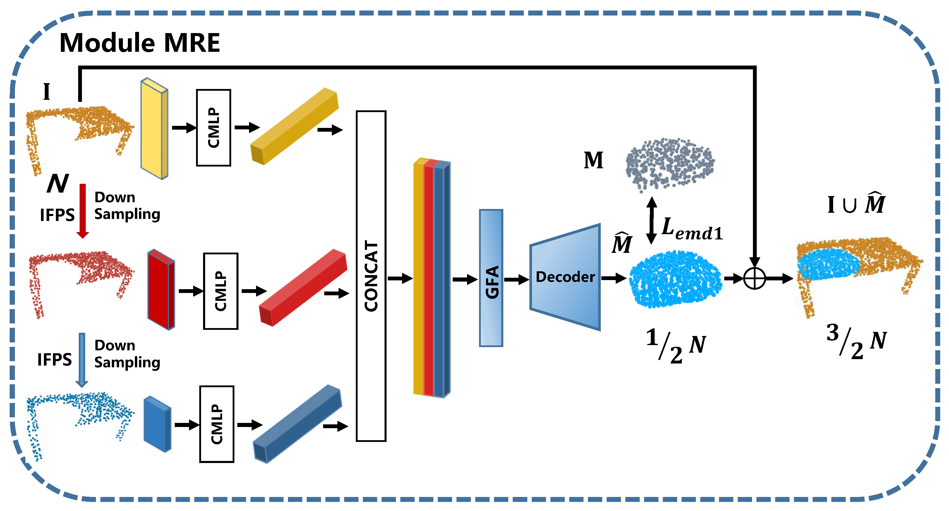
3.1.2. Multi-Resolution Encoder

The architecture of 3DPCTN-MRE is shown in Figure 4. We first introduce the feature extractor of 3DPCTN-MRE, namely, combined multi-layer perception (CMLP). Conventionally, the feature extractor in the encoder is to use a multi-layer perceptron (MLP) structure similar to PointNet. This type of method maps each point to a three-dimensional space, and extracts the maximum value from the final multi-dimensions to form a global feature vector. However, this type of method does not make good use of the rich local information of the low-level and middle-level features. In the CMLP [15], MLP is also used to encode each point of the point cloud into multiple dimensions [64, 64, 128, 256, 512, 1024]. Differently to PointNet, CMLP performs max pooling on the output of the last four layers of MLP to obtain a multi-dimensional feature vector $f_i$, where the dimensions of $f_i$ are [128, 256, 512, 1024], $i=1,\cdots ,4$. Then, we connect all the multi-dimensional features to form a combined feature vector $F_j$, which can be represented as:

$$F_j=concat(f_1,f_2,f_3,f_4),j=1,2,3$$

(6)

where the dimension of $F_j$ is 1920, which contains both low-level and high-level feature information.

The input of multi-resolution encoder is also an $N\times 3$ unordered point cloud. We sample the input point cloud by IFPS to obtain two other scales with different resolutions, where the sizes are $(N⁄x)\times 3$ and $(N⁄x^2)\times 3$ ($x=2$ in the experiments). Since applying these three incomplete point clouds with different resolutions into three CMLPs will lead to three sets of features with different resolutions, we use the above MRE data-dependent method to obtain the feature points of different input scale-point sets to help the encoder focus on those more representative points. These three point clouds with different resolutions will be mapped to three independent combined-feature vectors $F_j$ by CMLP, where $j=1,2,3$. Each vector $F_j$ represents the features extracted from the point cloud at a certain resolution of [2048, 1024, 512]. Then all $F_j$ are connected to form a dimension of $1920\times 3$, which is expressed as $F_o$:

$$\begin{array}{c}{F}_o=concat(F_1,F_2,F_3).\end{array}$$

(7)

Then, we use MLP to integrate the feature-vector mapping into the global feature vector $F_g$, whose size is 1920:

$$\begin{array}{c}{F}_g=MLP\left(F_o\right).\end{array}$$

(8)

3.1.3. Missing-Part Network Decoder

The decoder converts the feature vector $F_g$ into the required missing-part point cloud. The dimension of the missing part of the point cloud to be output is expressed as $X\times 3$, $(X=1⁄2N)$. To improve the overall architecture performance, morph-based decoder (MBD) is used as the decoder; the architecture is described in Ref. [14]. The decoder consists of K (as per setting in Ref. [14], $K=16$) surface morph-based networks to generate complex shapes. It is expected that the shape of each surface generated by the morph-based network will be concentrated on a relatively simple local area, thus making the generation of local surfaces easier. Therefore, the MBD is more suitable for our goal of generating partially missing point clouds. Each element of the network output is a map of a 2D square to a 3D surface. Each 2D surface is randomly extracted from the unit square ${[0,1]}^2$, and then an MLP is used to map them to a 3D surface. The perceptron is used to mimic a 2D square morphing into a 3D surface. In each forward transmission, we randomly sample $X⁄K$ points from the unit square. Then, before passing feature as an input to the K MLPs, we first connect the feature vector $F_g$ with the 2D point. Each sampled 2D point will be mapped to K 3D points located on K different surface elements. As a result, point cloud with a predicted shape of $K·X⁄K=X$ points is output in each forward direction. Since MLP learns continuous mapping from 2D to 3D, the decoder can generate a smooth surface by densely sampling on 2D, and this method can combine the results of multiple forward passes to generate point clouds with arbitrary resolutions.

Since the MLP in AtlasNet does not explicitly prevent the generation of point clouds with the same coordinates, overlap or excessive dispersion between surface point clouds are inevitable. This can also cause surface elements to expand and cover a larger area, which makes it more difficult to deform 2D squares and capture local details. To this end, we use an expansion penalty loss $L_{expansion}$ [14] as a regularizer for surface elements. It makes every surface element compact and concentrated in a local area. As the expansion penalizes loss, the overlap between the surface elements is reduced. Therefore, it allows each surface element to generate a more flexible shape. Finally, the size of the missing-part point cloud $\widehat{M}$ predicted by the encoder is $1⁄2\times N\times 3$.

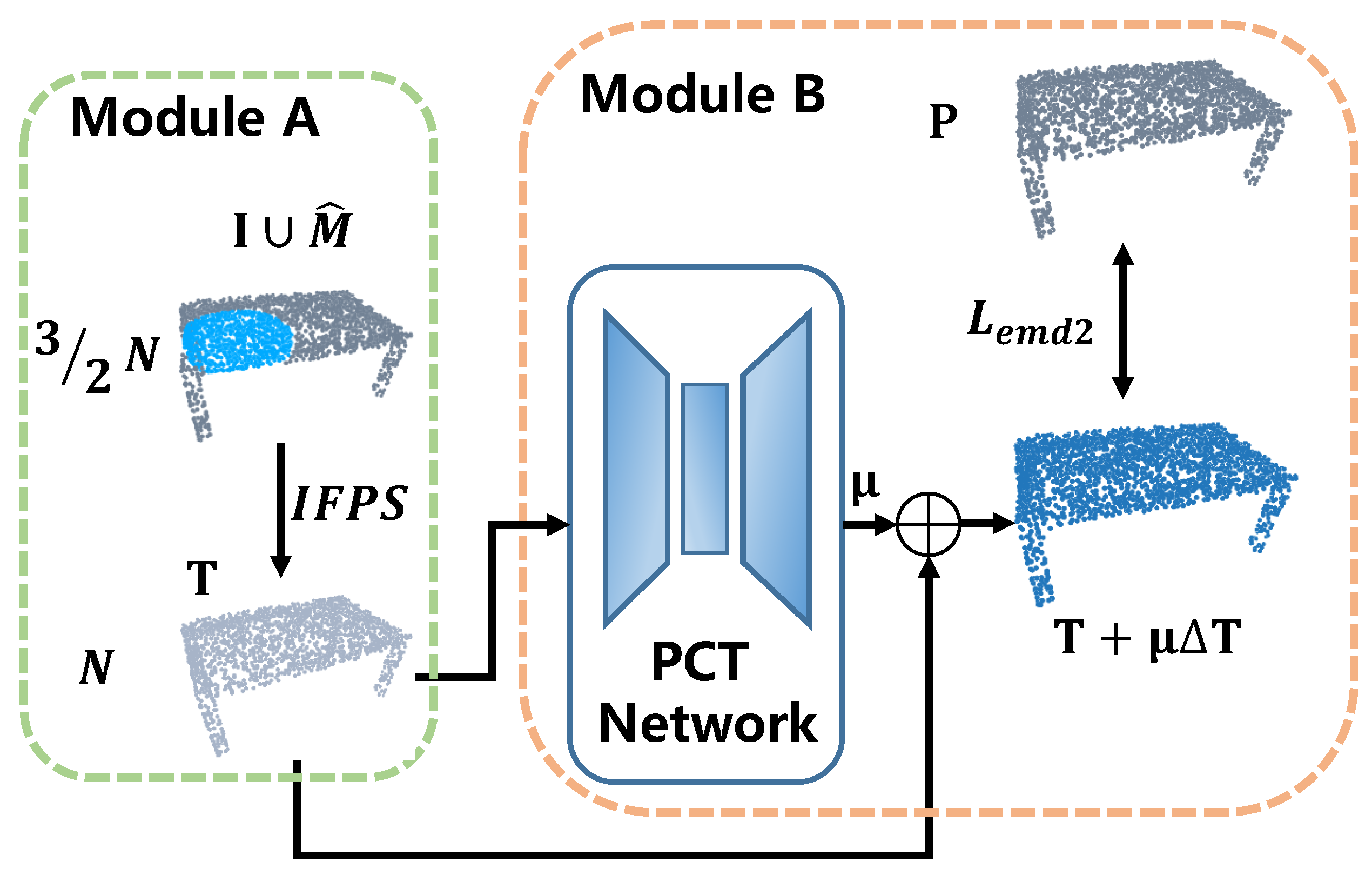
3.2. Merging and Sampling

Using an MBD, we can generate a smooth point cloud that predicts the shape of the missing part. However, due to its limited capabilities, the decoder may ignore certain structures, such as relatively subtle shapes that cannot be reconstructed, incomplete point cloud I and the predicted missing part of the point cloud $\widehat{M}$ with different densities and uneven distributions. The uniformity problem will make the final merged structure unrealistic. At the same time, fixed-size surface elements are not flexible enough for fine-grained local details.

By connecting the input point cloud I to the missing part of the point cloud $\widehat{M}$ and the result of the connection is a point cloud $I\cup \widehat{M}$ with a size of $3/2\times N\times 3$, we realize that there are two problems with the connection. First, the density of the missing part of the point cloud $\widehat{M}$ is higher than the density of the input point cloud I, because the missing part of the point cloud $\widehat{M}$ is only a small area, but there is half number of the points to the input point cloud I. Secondly, the size of our spliced point cloud does not match the size of the ground truth. To solve these problems, we use sampling methods to adjust the point distribution and the size of the merged point cloud. Since the density of the two point clouds may be different and they may overlap, the merged point cloud may be unevenly distributed. Therefore, we hope to sample a subset of point clouds with a uniform distribution from the combination. Thus, we use IFPS, as it has been effectively applied in PointNet++ [12]. After sampling $I\cup \widehat{M}$ using IFPS, T with a size of N is obtained. The architecture of our merging and sampling is shown in Module A of Figure 5.

3.3. Point-Refiner Network (PRN)

As a concatenation of the incomplete input I and the missing part of the prediction $\widehat{M}$ may create a visible gap in the final point cloud, the goal of our refining network is to solve this problem by smoothing the transition between the two merged point clouds. In addition, the refined network can also enhance the final distribution of the point cloud in the object. Module B in Figure 5 shows the abbreviated structure of the PRN. It mainly contains PCT modules. The architecture of the PCT is shown in Figure 6.

The encoder in PCT functions similar to the SAE in self-attention encoder, but the global feature vector is not just $F_o$ pass MP. The maximum feature vector $F_m$ and the average feature vector $F_a$ will be generated by $F_o$, respectively, fed-MP and average-pooling (AP) learning. Specifically, we choose to connect the output of two pooling operators: MP and AP operator in the cloud-point-feature-representation learning process. Both the maximum pooling feature and the average pooling features are repeated N times, then we connect them to obtain the global feature $F_g$. Next, we connect the global feature $F_g$ with the point-wise feature $F_o$, and then obtain the final completed point cloud after three one-dimensional convolutions. At this stage, we move the predicted missing part of the point cloud to a reasonable position, which preserves the completeness of the features of the original predicted missing part of the point cloud.

PRN is to learn a parameter function to improve the sampled point set T. We use the PCT network to predict the displacement $▵T$ to move T to a more desirable position to improve the distribution of points within T. The final output is a point cloud $T+\mu ▵T$, where $\mu \in [0,1]$ is a hyper-parameter that controls the amount of displacement we intend to maintain. In our experiments, $\mu =0.15$, which ensures that the shape of the original point cloud is not seriously changed. The displacement $▵T$ is obtained by using the PCT network.

3.4. Loss Function

The existing similarity indicators mainly include chamfer distance (CD) and earth mover’s distance (EMD). For two point clouds $S_1$ and $S_2$, CD measures the average distance from each point in $S_1$ to the nearest neighbor in $S_2$ space, added with the average distance from each point in $S_2$ to the nearest point in $S_1$ space.

$$\begin{array}{c}\hfill L_{CD}(S_1,S_2)=\frac{1}{2}\left(\frac{1}{S_1}{\Sigma }_{x\in S_1}\underset{y\in S_2}{min}\parallel x-y\parallel \right)+\frac{1}{S_2}{\Sigma }_{y\in S_2}\underset{x\in S_1}{min}\parallel x-y\parallel ).\end{array}$$

(9)

In contrast, EMD is a metric between two distributions, only when $S_1$ and $S_2$ have the same size, based on the minimum cost of converting one distribution to the other. Given two point clouds of the same size, the definition of EMD is as follows:

$$L_{EMD}(S_1,S_2)=\underset{\phi :S_1\to S_2}{min}\frac{1}{S_1}{\Sigma }_{x\in S_1}{\parallel x-\phi \left(x\right)\parallel }_2,$$

(10)

where $\phi$ is a bijective function. Due to the lower computational cost of CD, most of the existing works use CD as their loss function. However, CD turned a blind eye to certain visual disadvantages. The output points of general point-cloud autoencoders are often over-filled in parts of huge volume, i.e., the top of a table, and the details of the variable part are always blurred. However, it is difficult for CD to penalize this type of deception, because one of these types of deception may increase very little, and the other may be negligible.

EMD provides better reconstruction results attributed to its one-to-one mapping. By solving the linear-distribution problem, EMD forces the output to have the same density distribution as the ground-truth value, so that the local details and density distribution have better fidelity. In our paper, we use the EMD implemented in [14], which has an $O\left(n\right)$ memory footprint and takes up less computational cost.

In the proposed architecture, we calculated the losses of both the missing-part prediction network and the point-refiner network. The first loss calculates the EMD between the predicted missing point cloud $\widehat{M}$ and the missing ground truth point cloud M. The second loss is the EMD between the more refined point cloud $\widehat{P}$ and the completed ground-truth point cloud P. Our final joint loss can be expressed as:

$$L=L_{EMD}(\widehat{M},M)+L_{expansion}+L_{EMD}(\widehat{P},P).$$

(11)

The EMD term and the extended penalty work in opposite directions. The former encourages the point cloud to cover the shape of the entire object; the latter, as an adjustment, encourages each surface element to shrink. The mutual restraint allows each surface element to be concentrated in a local area, each element stays as close as possible to the ground-truth value.

4. Experimental Results and Analysis

4.1. Data Generation and Implementation Details

Our evaluation method uses the protocol [16]. To train our model, we use 13 categories of different objects in the benchmark dataset ShapeNet-Part [30]. The dataset consists of 13 categories in the ShapeNet-Part dataset: Airplane, Bag, Cap, Car, Chair, Guitar, Lamp, Laptop, Motorbike, Mug, Pistol, Skateboard and Table. The data set contains 14,473 models (11,705 for training and 2768 for testing). Before using these point-cloud models, we first standardize their position and scale. As the position and scale are standardized, we move the center of all input point clouds to the origin, and then normalize the input point-cloud data to $[-1,1]$; that is, we normalize the data to a radius of 1. Finally, we uniformly sample each point-cloud model into 2048 points to create ground-truth point-cloud data.

In each epoch, we generate an incomplete point cloud from the completed point-cloud model. Incomplete point-cloud data is usually generated by randomly selecting a perspective from multiple views, then randomly selecting a point as the center, and deleting all points within a sphere of a certain radius r from the completed point cloud. We control the radius to obtain missing data with different sizes, and the size of r is 0.35 in our experiment. As shown in the experiments in Section 4.3, all methods have better results when the radius is 0.35. Hence, our completed point cloud can be divided into two groups: points outside the sphere (incomplete point cloud) and points inside the sphere (missing point cloud). Finally, we sample the originally completed point cloud as 2048 points to obtain the ground truth of the completed point cloud, sample 2048 points from the original incomplete point cloud as the input in the experiment, and sample 1024 points from the original missing-part point cloud as the ground truth of the missing part in the experiment. It should be noted that, in 3DPCTN-MRE, in addition to generating incomplete point clouds, we also need to perform IFPS sampling on incomplete input point clouds to obtain two additional scales with different resolutions; therefore, in the 3DPCTN-MRE experiment, our incomplete point-cloud input has three different resolution scales, namely, 2048, 1024 and 512.

4.2. Comparsions with State-of-the-Art Methods

In this section, we compare our method with several representative benchmarks that run directly on 3D point clouds, including 3D point-capsule networks (3D-Capsule) [26], PCN [16], morphing and sampling Network (MSN) [14], PF-Net [15], and RP-MBD [31], which are briefly introduced as follows:

• 3D-Capsule uses the most advanced autoencoder to process point clouds for point-cloud reconstruction, which is based on a capsule network.
• PCN completes a partial point cloud by an autoencoder. It uses a stacked version of PointNet as the encoder and generates the point cloud in a coarse-to-fine form.
• MSN is generated using two stages, first predicting the coarse point cloud, and then using the residual network to further enhance for obtaining a high-density point cloud.
• PF-Net learns multi-scale features from local shapes and regenerates missing parts at different resolutions. Additionally, an adversarial loss is included to match the distribution of predicted and actual missing regions.
• RP-MBD consists of two PointNet-based networks. The first network is based on focusing on extracting information from incomplete inputs to infer missing geometries, and the other network merges two point clouds and improves point distribution.

ShapeNet-Part test datasets are used for quantitative and qualitative comparisons. We have trained and tested all methods using the same dataset to perform fair quantitative evaluations.

The quantitative results for the comparison are shown in

Table 1. Quantitative comparison between our methods and existing methods on ShapeNet-Part dataset using chamfer distance (CD × 1000) with 2048 points. The best results are highlighted in bold.

Categories	3D-Capsule	PCN	MSN	PF-Net	RP-MBD	3DPCTN-SAE	3DPCTN-MRE
Airplane	2.277	1.579	0.661	0.533	0.467	0.325	0.326
Bag	6.501	4.872	2.333	2.252	1.670	0.598	0.580
Cap	6.939	5.782	2.266	1.927	1.109	0.408	0.390
Car	5.467	3.882	1.543	0.853	0.946	0.655	0.597
Chair	4.496	2.560	1.036	0.745	0.663	0.396	0.395
Guitar	3.741	0.809	0.859	0.437	0.381	0.280	0.390
Lamp	9.258	5.466	2.969	2.358	2.325	1.489	1.527
Laptop	2.565	1.708	0.745	0.516	0.379	0.335	0.305
Motorbike	4.770	3.121	1.398	0.854	1.084	0.784	0.804
Mug	6.219	5.108	1.453	1.025	0.743	0.644	0.546
Pistol	3.411	2.277	1.144	0.855	0.867	0.546	0.547
Skateboard	3.015	1.923	0.720	0.571	0.454	0.332	0.308
Table	4.099	2.982	1.196	1.071	0.833	0.400	0.424
Average	4.827	3.236	1.409	1.077	0.917	0.553	0.549

and

Table 2. Quantitative comparison between our methods and existing methods on ShapeNet-Part dataset using earth mover’s distance (EMD × 100) with 2048 points. The best results are highlighted in bold.

Categories	3D-Capsule	PCN	MSN	PF-Net	RP-MBD	3DPCTN-SAE	3DPCTN-MRE
Airplane	4.038	4.122	2.078	1.474	1.394	1.131	1.119
Bag	7.480	8.263	3.903	2.199	2.438	1.863	1.723
Cap	6.818	7.224	3.299	1.937	2.074	1.382	1.438
Car	6.157	5.953	3.336	1.758	2.140	1.733	1.701
Chair	5.322	5.646	2.439	1.575	1.638	1.318	1.288
Guitar	3.769	3.866	2.107	1.528	1.234	1.103	1.232
Lamp	8.535	7.798	3.603	2.588	2.848	2.235	2.233
Laptop	4.303	4.068	2.180	1.428	1.435	1.312	1.268
Motorbike	6.005	5.769	3.295	2.183	2.291	1.936	1.989
Mug	6.822	7.226	2.780	1.620	1.628	1.622	1.519
Pistol	4.873	4.994	2.643	2.034	1.938	1.521	1.502
Skateboard	4.309	4.035	1.958	1.509	1.341	1.103	1.100
Table	5.565	5.403	2.424	1.606	1.617	1.253	1.262
Average	5.692	5.720	2.772	1.803	1.847	1.501	1.490

. Both in CD and EMD metrics, 3DPCTN-SAE and 3DPCTN-MRE outperform the other methods in the mean of all categories and show significant improvement in all categories. The error of the completed point cloud as a whole may come from two parts: the prediction error of the missing area and the change in the original local shape. Since our method takes a part of the shape as input and outputs only the missing region, it basically does not change the original part of the shape. In both CD and EMD metrics, 3DPCTN-MRE outperforms 3DPCTN-SAE in most categories. Our method performs well even for the harder classes in the dataset, such as Bag, Cap and Lamp. The problem with the Bag and Cap classes is the imbalanace in the number of shapes in the dataset (Bag contains 54 training shapes and Cap contains 39 training shapes), while the Lamp class has a problem with high intra-class variability. However, our method still has a strong performance in these categories compared to other methods. This is mainly due to the combined advantage of missing-part prediction and refinement in our method: for the challenging classes, the prediction of the missing point cloud will first compute a rough output, which is then corrected by refinement.

Visual comparison in Figure 7 and Figure 8 demonstrate that our 3DPCTN also achieves much better visual results than the other counterparts on the sparse point-cloud completion task. All the methods are relatively good in the complete effect of simple objects, such as the chair in the third column, but in more complex cases, the difference in methods is obvious. Specifically, for 3D-Capsule and PCN, since the encoder–decoder-based feature extraction and full point-cloud generation use fully connected layers to directly output coordinates, they tend to generate ambiguous details such as Plane and Cap. For MSN, although it is based on the first rough and then refined generative model, and then uses the residual network to optimize it, only the global features of the input residual fault cloud are extracted in the early stage, so some detailed information, such as Chair and Cup, will be lost. In the Lamp category, 3DPCTN is the only way to reconstruct the missing light posts without any noticeable noise. The Pistol highlights the obvious advantage of generating only the missing parts, rather than recreating the entire shape, and also shows how the 3DPCTN is more accurate than the PF-Net and RP-MBD.

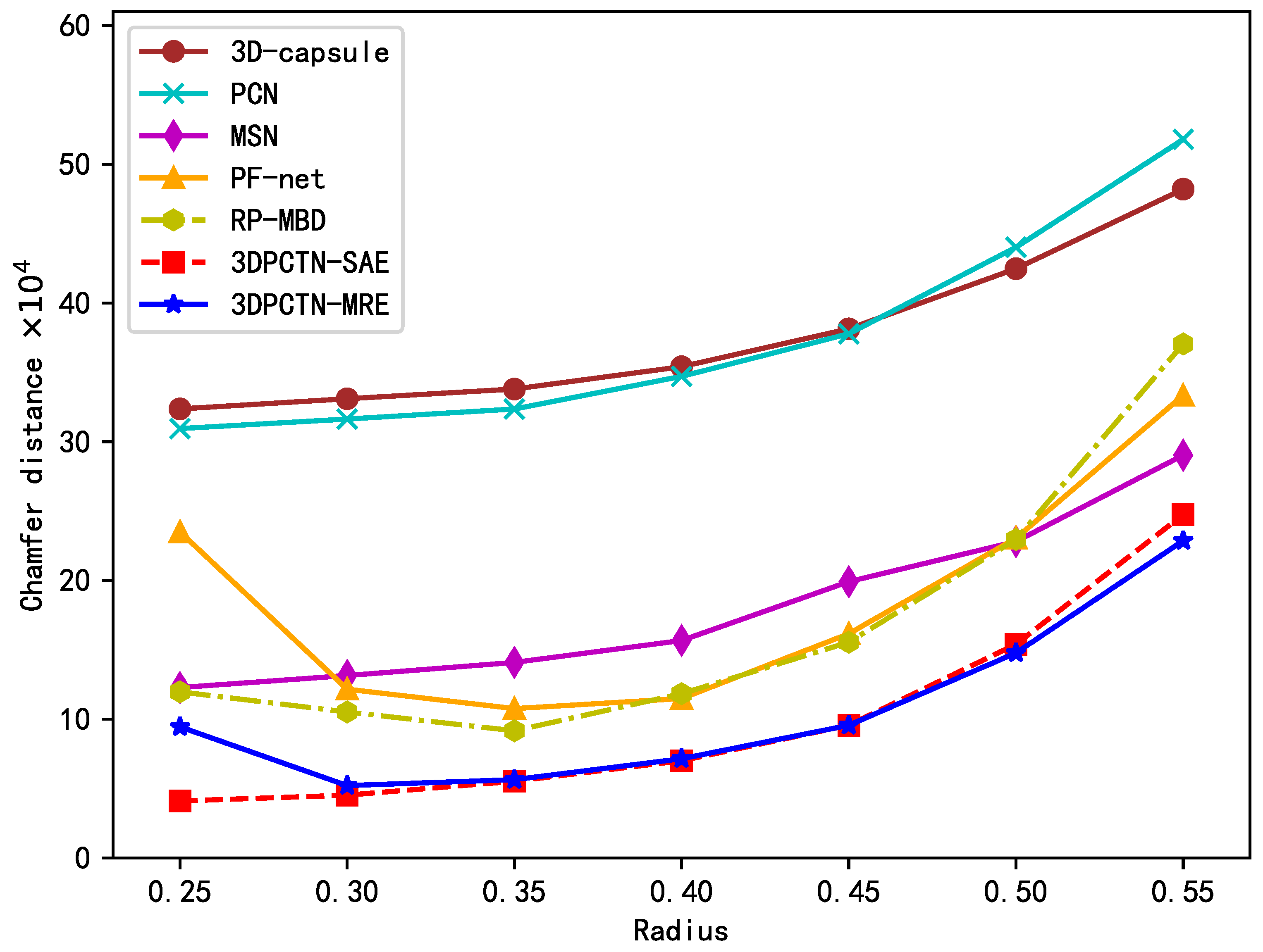
4.3. Robustness Test

In this robustness test experiment, our purpose is to evaluate the robustness of our proposed model with some point clouds with missing holes of a different radius. The model used in this experiment is the same as the model compared in Section 4.2, except that the radius of the missing part of the incomplete point cloud that needs to be completed in this test is different. In the previous comparison, we used a radius of 0.35. However, when the test shape has missing parts of different sizes, we measure the robustness of the model to completion. We change the radius from 0.25 to 0.55 and calculate the average chamfer distance for each algorithm.

Figure 9 shows the results. When the size of the missing part varies between 0.25 and 0.45, our method is always better than other methods. Our method always performed better than other methods. That is, our method of predicting the completed point cloud shows better robustness. When the radius increases, the performance of all methods generally shows a downward trend; especially, when the radius is greater than 0.5, the performance decline is greater. We believe that the reason for the decrease in the robustness of all methods is that our fixed number of points cannot cover and represent the missing parts. One of the main limitations of our method is the lack of adaptability and the inability to express the missing part according to the extent of the proportions that are missing. It is a promising idea to calculate an adaptive variable size point cloud through a neural network, which can be incorporated into our method to improve robustness.

4.4. Ablation Study

The performance improvement of 3DPCTN should be attributed to three key components, SAE, MRE and PCT. To prove the effectiveness of each component in the proposed method, we evaluated the 3DPCTN performance using the same parameters as Section 4.2. In this experiment, we demonstrated the importance of these key components to the point-cloud completion results. Furthermore, the contribution of each component could be verified by deleting any components that will reduce performance. Comparison results between different ablation methods are listed in

Table 3. Quantitative comparison between our method and the ablated versions on ShapeNet-Part dataset using chamfer distance (CD × 1000) with 2048 points. The best results are highlighted in bold and underlined. The lower results are the better.

Categories	3DPCTN-SAE	3DPCTN-SAE w/o PCT	3DPCTN-MRE	3DPCTN-MRE w/o PCT	Only PCT w/o SAE and MRE
Airplane	0.325	0.493	0.326	0.448	0.329
Bag	0.598	1.375	0.580	1.305	0.610
Cap	0.408	1.092	0.390	0.85	1.300
Car	0.655	1.080	0.597	0.857	0.632
Chair	0.396	0.701	0.395	0.622	0.404
Guitar	0.280	0.724	0.390	0.33	0.334
Lamp	1.489	7.157	1.527	2.275	1.550
Laptop	0.335	0.522	0.305	0.379	0.323
Motorbike	0.784	0.926	0.804	0.925	0.784
Mug	0.644	0.646	0.546	0.779	0.626
Pistol	0.546	0.702	0.547	0.736	0.575
Skateboard	0.332	0.428	0.308	0.436	0.314
Table	0.400	0.638	0.424	0.764	0.438
Average	0.553	1.271	0.549	0.824	0.632

.

In the experimental results of the PCT importance test, the comparison between the second column and the third column, and the comparison between the fourth column and the fifth column, are worthy of attention. From the bold fonts (the ones with bold fonts are the best), it is obvious that the two experimental results of the PCT method are almost excellent whether in the SAE or MRE networks. Moreover, the average of all categories is much better than the result without PCT. When testing the significance of SAE and MRE, we observed the second and sixth columns, and the fourth and sixth columns, respectively, and found that both SAE and MRE can also reduce the CD value of the complete shape after completion. In addition, the average reduction in each category is relatively large. Overall, the PCT, SAE and MRE modules play an integral role in our proposed network.

5. Conclusions

In this paper, we have presented a novel neural network for point-cloud completion called 3DPTCN, which completes the original point cloud in three stages. Furthermore, 3DPTCN extracts fine-grained point-cloud features from self-attention and multi-resolution, respectively, and can effectively control point distribution using the expansion penalty during point-cloud generation. The PCT-based point-refiner network is used to predict the fine tuning of each point to achieve fine-grained details while preserving the original shape. We conducted comprehensive experiments on the ShapeNet-Part dataset, which show that our 3DPTCN is superior to the current SOTA point-cloud completion method and produces more uniform point clouds. In future work, we will work on adaptive strategies to compute missing dimensions to improve the complete performance of our network.

References

1. Chen, T.; Lin, L.; Hui, X.; Chen, R.; Wu, H. Knowledge-guided multi-label few-shot learning for general image recognition. IEEE Trans. Pattern Anal. Mach. Intell. 2020, 44, 1371–1384. [Google Scholar] [CrossRef]
2. Chen, T.; Pu, T.; Wu, H.; Xie, Y.; Liu, L.; Lin, L. Cross-domain facial expression recognition: A unified evaluation benchmark and adversarial graph learning. IEEE Trans. Pattern Anal. Mach. Intell. 2021. [Google Scholar] [CrossRef] [PubMed]
3. Yang, Z.; Wang, L. Learning relationships for multi-view 3D object recognition. In Proceedings of the IEEE/CVF International Conference on Computer Vision, Seoul, Korea, 27–28 October 2019; pp. 7505–7514. [Google Scholar] [CrossRef]
4. Wei, X.; Yu, R.; Sun, J. View-GCN: View-based graph convolutional network for 3D shape analysis. In Proceedings of the IEEE/CVF Conference on Computer Vision and Pattern Recognition, Seattle, WA, USA, 13–19 June 2020; pp. 1850–1859. [Google Scholar]
5. Maturana, D.; Scherer, S. Voxnet: A 3d convolutional neural network for real-time object recognition. In Proceedings of the 2015 IEEE/RSJ International Conference on Intelligent Robots and Systems (IROS), Hamburg, Germany, 28 September–2 October 2015; pp. 922–928. [Google Scholar]
6. Riegler, G.; Osman Ulusoy, A.; Geiger, A. Octnet: Learning deep 3d representations at high resolutions. In Proceedings of the IEEE Conference on Computer Vision and Pattern Recognition, Honolulu, HI, USA, 21–26 July 2017; pp. 3577–3586. [Google Scholar]
7. Le, T.; Duan, Y. Pointgrid: A deep network for 3d shape understanding. In Proceedings of the IEEE Conference on Computer Vision and Pattern Recognition, Salt Lake City, UT, USA, 18–23 June 2018; pp. 9204–9214. [Google Scholar]
8. Wang, N.; Zhang, Y.; Li, Z.; Fu, Y.; Liu, W.; Jiang, Y.G. Pixel2mesh: Generating 3d mesh models from single rgb images. In Proceedings of the European Conference on Computer Vision (ECCV), Munich, Germany, 8–14 September 2018; pp. 52–67. [Google Scholar]
9. Zeng, W.; Ouyang, W.; Luo, P.; Liu, W.; Wang, X. 3d human mesh regression with dense correspondence. In Proceedings of the IEEE/CVF Conference on Computer Vision and Pattern Recognition, Seattle, WA, USA, 13–19 June 2020; pp. 7054–7063. [Google Scholar]
10. Zhu, H.; Zuo, X.; Wang, S.; Cao, X.; Yang, R. Detailed human shape estimation from a single image by hierarchical mesh deformation. In Proceedings of the IEEE/CVF Conference on Computer Vision and Pattern Recognition, Long Beach, CA, USA, 15–20 June 2019; pp. 4491–4500. [Google Scholar]
11. Qi, C.R.; Su, H.; Mo, K.; Guibas, L.J. Pointnet: Deep learning on point sets for 3d classification and segmentation. In Proceedings of the IEEE Conference on Computer Vision and Pattern Recognition, Honolulu, HI, USA, 21–26 July 2017; pp. 652–660. [Google Scholar]
12. Qi, C.R.; Yi, L.; Su, H.; Guibas, L.J. Pointnet++: Deep hierarchical feature learning on point sets in a metric space. arXiv 2017, arXiv:1706.02413. [Google Scholar]
13. Wu, H.; Miao, Y.; Fu, R. Point cloud completion using multiscale feature fusion and cross-regional attention. Image Vis. Comput. 2021, 111, 104193. [Google Scholar] [CrossRef]
14. Liu, M.; Sheng, L.; Yang, S.; Shao, J.; Hu, S.M. Morphing and sampling network for dense point cloud completion. In Proceedings of the AAAI Conference on Artificial Intelligence, New York, NY, USA, 7–12 February 2020; Volume 34, pp. 11596–11603. [Google Scholar]
15. Huang, Z.; Yu, Y.; Xu, J.; Ni, F.; Le, X. Pf-net: Point fractal network for 3d point cloud completion. In Proceedings of the IEEE/CVF Conference on Computer Vision and Pattern Recognition, Seattle, WA, USA, 13–19 June 2020; pp. 7662–7670. [Google Scholar]
16. Yuan, W.; Khot, T.; Held, D.; Mertz, C.; Hebert, M. Pcn: Point completion network. In Proceedings of the 2018 International Conference on 3D Vision (3DV), Verona, Italy, 5–8 September 2018; pp. 728–737. [Google Scholar]
17. Xie, H.; Yao, H.; Zhou, S.; Mao, J.; Zhang, S.; Sun, W. Grnet: Gridding residual network for dense point cloud completion. In Proceedings of the European Conference on Computer Vision, Glasgow, UK, 23–28 August 2020; pp. 365–381. [Google Scholar]
18. Tchapmi, L.P.; Kosaraju, V.; Rezatofighi, H.; Reid, I.; Savarese, S. Topnet: Structural point cloud decoder. In Proceedings of the IEEE/CVF Conference on Computer Vision and Pattern Recognition, Long Beach, CA, USA, 15–20 June 2019; pp. 383–392. [Google Scholar]
19. Wang, X.; Ang Jr, M.H.; Lee, G.H. Cascaded refinement network for point cloud completion. In Proceedings of the IEEE/CVF Conference on Computer Vision and Pattern Recognition, Seattle, WA, USA, 13–19 June 2020; pp. 790–799. [Google Scholar]
20. Guo, M.H.; Cai, J.X.; Liu, Z.N.; Mu, T.J.; Martin, R.R.; Hu, S.M. PCT: Point cloud transformer. arXiv 2020, arXiv:2012.09688. [Google Scholar] [CrossRef]
21. Yuan, M.; Li, X.; Cheng, L.; Li, X.; Tan, H. A Coarse-to-Fine Registration Approach for Point Cloud Data with Bipartite Graph Structure. Electronics 2022, 11, 263. [Google Scholar] [CrossRef]
22. Fan, H.; Su, H.; Guibas, L.J. A point set generation network for 3d object reconstruction from a single image. In Proceedings of the IEEE Conference on Computer Vision and Pattern Recognition, Honolulu, HI, USA, 21–26 July 2017; pp. 605–613. [Google Scholar]
23. Achlioptas, P.; Diamanti, O.; Mitliagkas, I.; Guibas, L. Learning representations and generative models for 3d point clouds. In Proceedings of the International Conference on Machine Learning, Stockholm, Sweden, 10–15 July 2018; pp. 40–49. [Google Scholar]
24. Yang, Y.; Feng, C.; Shen, Y.; Tian, D. Foldingnet: Point cloud auto-encoder via deep grid deformation. In Proceedings of the IEEE Conference on Computer Vision and Pattern Recognition, Salt Lake City, UT, USA, 18–23 June 2018; pp. 206–215. [Google Scholar]
25. Groueix, T.; Fisher, M.; Kim, V.G.; Russell, B.C.; Aubry, M. A papier-mâché approach to learning 3d surface generation. In Proceedings of the IEEE Conference on Computer Vision and Pattern Recognition, Salt Lake City, UT, USA, 18–23 June 2018; pp. 216–224. [Google Scholar]
26. Zhao, Y.; Birdal, T.; Deng, H.; Tombari, F. 3D point capsule networks. In Proceedings of the IEEE/CVF Conference on Computer Vision and Pattern Recognition, Long Beach, CA, USA, 15–20 June 2019; pp. 1009–1018. [Google Scholar]
27. Zhao, H.; Jiang, L.; Jia, J.; Torr, P.; Koltun, V. Point transformer. arXiv 2020, arXiv:2012.09164. [Google Scholar]
28. Zhao, H.; Jia, J.; Koltun, V. Exploring self-attention for image recognition. In Proceedings of the IEEE/CVF Conference on Computer Vision and Pattern Recognition, Seattle, WA, USA, 13–19 June 2020; pp. 10076–10085. [Google Scholar]
29. Vaswani, A.; Shazeer, N.; Parmar, N.; Uszkoreit, J.; Jones, L.; Gomez, A.N.; Kaiser, Ł.; Polosukhin, I. Attention is all you need. In Proceedings of the Advances in Neural Information Processing Systems 30 (NIPS 2017), Long Beach, CA, USA, 4–9 December 2017; pp. 5998–6008. [Google Scholar]
30. Yi, L.; Kim, V.G.; Ceylan, D.; Shen, I.C.; Yan, M.; Su, H.; Lu, C.; Huang, Q.; Sheffer, A.; Guibas, L. A scalable active framework for region annotation in 3d shape collections. ACM Trans. Graph. (ToG) 2016, 35, 1–12. [Google Scholar] [CrossRef]
31. Mendoza, A.; Apaza, A.; Sipiran, I.; Lopez, C. Refinement of Predicted Missing Parts Enhance Point Cloud Completion. arXiv 2020, arXiv:2010.04278. [Google Scholar]
Figure 1. The overall point-cloud structure of the object is outputted directly from the trained neural network. Traditional approach tends to ignore the hollow pattern design on the backrest.
Electronics 11 01351 g001
Figure 2. Intuitive architecture of the proposed method. It consists of three modules: The missing-part prediction network uses an autoencoder structure to take the incomplete point cloud I as input and output the corresponding missing part M ^ . The merging and sampling module connects and samples the incomplete input cloud and the missing part of the prediction. The point-refiner network improves the distribution of point clouds and narrows the gap caused by merging.
Electronics 11 01351 g002
Figure 3. The 3DPCTN-SAE encoder mainly comprises an input-embedding module and four stacked attention modules. We connect the feature dimensions of the attention output of each attention layer, and then perform a linear transformation. Finally, a global feature of the missing part of the point cloud is obtained, which is fed into the missing-part network decoder to obtain a completed shape point cloud M ^ .
Electronics 11 01351 g003
Figure 4. The 3DPCTN-MRE encoder first performs IFPS sampling on the input point cloud to obtain multi-scale features with resolution of [2048, 1024, 512]. Then, multi-scale feature representations are fed into the missing-part network decoder to obtain a completed shape point cloud M ^ .
Electronics 11 01351 g004
Figure 5. The architecture of our merging and sampling (Module A) and point-refiner network (Module B).
Electronics 11 01351 g005
Figure 6. The architecture of PCT. The encoder consists of an input-embedding module and four stacked attention modules. The decoder comprises multiple linear layers. MA-Pool concatenates MP and AP. LBR combines Linear, BatchNorm and ReLU layers. LBRD means LBR followed by a Dropout layer.
Electronics 11 01351 g006
Figure 7. Comparison of completion results between our method and state-of-the-art methods. Our 3DPCTN (3DPCTN-SAE and 3DPCTN-MRE) successfully predicts the missing part and integrates it to produce a good result.
Electronics 11 01351 g007
Figure 8. Comparison of completion results between our method and state-of-the-art methods. Our 3DPCTN (3DPCTN-SAE and 3DPCTN-MRE) successfully predicts the missing part and integrates it to produce a good result.
Electronics 11 01351 g008
Figure 9. Robustness against the variable size of missing parts. Our methods are robust when the size of the missing part is similar to the size of the trained missing part. A smaller value of CD indicates a better result.
Electronics 11 01351 g009