Communication

Learning Local Distribution for Extremely Efficient Single-Image Super-Resolution

School of Automation, Hangzhou Dianzi University, Hangzhou 310018, China
*
Author to whom correspondence should be addressed.
Electronics 2022, 11(9), 1348; https://doi.org/10.3390/electronics11091348
Submission received: 12 March 2022 / Revised: 14 April 2022 / Accepted: 19 April 2022 / Published: 24 April 2022
(This article belongs to the Topic Machine and Deep Learning)

Abstract

:
Achieving balance between efficiency and performance is a key problem for convolution neural network (CNN)-based single-image super-resolution (SISR) algorithms. Existing methods tend to directly output high-resolution (HR) pixels or residuals to reconstruct the HR image and focus a lot of attention on designing powerful CNN backbones. However, this reconstruction way requires the CNN backbone to have good ability to fit the mapping function from LR pixels to HR pixels, which certainly held these methods back from achieving extreme efficiency and from working in embedded environments. In this work, we propose a novel distribution learning architecture to estimate the local distribution and reconstruct HR pixels by sampling the local distribution with the corresponding 2D coordinates. We also improve the backbone structure to better support the proposed distribution learning architecture. The experimental results demonstrate that the proposed method achieves state-of-the-art performance for extremely efficient SISR and exhibits a good balance between efficiency and performance.

1. Introduction

Single image super-resolution (SISR) is a classic image processing task, which has been catching researchers’ attention for decades. The SISR targets reconstructing a high-resolution (HR) image with only one low-resolution (LR) image as input. Reconstructing clear and accurate edges is one of the major challenges in SISR.
Early studies focus on interpolation-based algorithms [1,2,3] that aim to calculate the sub-pixels with neighboring pixels.Due to the limited information on the neighboring pixels, interpolation-based methods fail to reconstruct visually clear edges. Introducing filtering-based methods for post-processing to enhance the interpolated image is another option [4,5]. These methods introduce non-local information [6] and non-linear filtering and certainly enhance the visual quality of the interpolated image. However, limited by the fronted interpolation methods, they also struggle to handle the large upsampling factors. The optimization-based methods introduce kinds of priors and approach the optimal results in an iterative way [7,8]. Limited by the complicated iterative solutions, these methods are usually quite inefficient. Moreover, because the statistical priors cannot fit all samples, the optimization-based methods also suffer from poor robustness. With the development of machine learning, lots of data-driven methods have been proposed [9,10,11]. The sparse coding-based methods [12,13,14] introduce a learning-based encoder to sparsely encode both LR patches and HR patches and then try to build the mapping function from LR patches to HR patches with sparse representation. However, the separated learning strategy and limited sparse representation certainly limit the performance of these methods.
Benefiting from the great growth of computation devices, deep-learning-based methods exhibit a promising performance, and some of them widely are adopted in the edge devices, such as surveillance cameras and mobile phones. Due to the power limitation and computational resource limitation, the efficiency is always firstly considered when deploying the algorithms to such edge devices.
Dong et al. [11] introduced a convolution neural network [15] and provided an end-to-end learning architecture named SRCNN for the SISR task. They first use bi-cubic interpolation to upsample the LR image to the target resolution and then introduce CNN to reconstruct the HR image from the upsampled LR image. In this situation, the CNN has to work on the upsampled images, which extends the time of calculation and is quite inefficient. Several studies [16,17] introduce transpose convolution [18] to conduct the upsampling operation within the CNN architecture. Some studies try to implement bi-linear interpolation within the CNN architecture to directly upsample the convolution feature map using bilinear interpolation. Due to the limited upsampling accuracy, these two operations could only work in the middle of the network. Therefore, parts of the convolution layers also have to work on the upsampled resolution. To overcome this limitation, Shi et al. [19] introduce a pixel shuffle operation and propose a sub-pixel learning network named ESPCN for SISR. Unlike previous studies that directly output the reconstructed HR image, ESPCN outputs the sub-pixels at each position and shuffle the sub-pixels to obtain the final HR image. By doing so, the upsampling operation is moved to the end of the network, so that the whole CNN could work on the original resolution.
Then, lots of studies adopted the pixel shuffle operation to reconstruct the HR pixels and focus on the powerful and efficient backbone to achieve a balance between performance and efficiency. Increasing the depth and introducing more components are general ways to obtain more powerful backbones [20,21]. Introducing and optimizing the residual-like components are widely adopted in relative research [22,23]. Liu et al. [24] propose a residual feature aggregation (RFA) framework to aggregate these informative residual features to produce more representative features. Zhang et al. [25] propose a context reasoning attention network (CRAN) to adaptively modulate the convolution kernel according to the global context for the SISR task. Zhang et al. [26] propose an end-to-end trainable unfolding network that leverages both learning-based methods and model-based methods. The network inherits the flexibility of model-based methods while maintaining the advantages of learning-based methods. Other studies [27,28] introduce a Generative Adversarial Network (GAN) to process real-world LR images, which are do not perform well based on CNN methods.
Though these methods could significantly improve the performance, they are hardly deployed on hardware platforms [29,30] because of the extreme efficiency requirement. In this paper, we rethink the SISR task along the signal sampling direction and propose a CNN-based local distribution reconstruction network (LDRN) for an extremely efficient SISR task, aiming to provide a new baseline for hardware platforms.
The LDRN first introduces a neural network model to reconstruct the distribution of the neighbor area of each LR pixel and then calculates the sub-pixels within the neighboring area based on their relative coordinates from the center pixel. Compared to existing methods, the proposed method achieves an excellent balance in efficiency and performance, exhibiting good potential for being deployed to hardware platforms.

2. Proposed Method

Given a scene and a camera lens, the resolution of the captured image depends on the number of photosensitive cells on the image sensor. Increasing the density of the photosensitive cells is a direct way to increase the resolution of the captured image. Assuming the real signal distribution of the scene is D , the sampling matrix of the image sensor is M , and the captured image I can be expressed as:
I = S ( D , M ) ,
where S denotes a sampling function. Therefore, changing the sampling matrix M directly affects the resolution of the captured image. Because M is always uniformly arranged, the corresponding sampling matrix of an HR image M H R can be easily calculated. Therefore, the keypoint of calculating the HR image from an LR image is reconstructing the scene’s distribution D .

2.1. Motivation

A static natural scene is a 3D signal. After the optic transformation is conducted by the camera lens, the scene’s signal degrades to a 2D signal S ( x , y ) lying on the image plane. Because the S ( x , y ) totally depends on the scene, it is hard to give a specific mathematical model to describe the S ( x , y ) . We try to decompose the S ( x , y ) into multiple patches and reconstruct the local distribution of each patch for sub-pixel reconstruction.
Because all observed pixels are uniformly arranged, we set the horizontal (or vertical) distance between two adjacent pixels in the LR image as the unit length. Then, given a image patch P with the size of 2 ω × 2 ω , whose center is located at ( x P , y P ) , its local distribution can be expressed as:
S P , ω ( x , y ) = L ( x x P , y y P ; H P )
where x [ x ω , x + ω ] , y [ y ω , y + ω ] , L denotes a parameterized mathematical model to describe the local distribution, and H P denotes the corresponding parameters to formulate L .
Assuming the sampling points in the HR image are { ( x p 1 , y p 1 ) , ( x p 2 , y p 2 ) , , ( x p k , y p k ) } , we can easily calculate all observed pixels with Equation (2). Given a specific upsampling factor s and the corresponding matrix M s , the observed k HR pixels of the corresponding region of the LR patch P can be quickly located in M s . Enlarging the patch size and conducting the overlapped calculation are widely adopted by traditional methods [31]. However, such strategy is quite inefficient in CNN-based methods. Inspired by [19], we adopt a pixel-wise local reconstruction strategy. As shown in Figure 1, each local patch contains one pixel in the LR image and the corresponding sub-pixel in the HR image. In this way, the reconstruction area and sampling points are both minimized, which could significantly simplify the local distribution reconstruction and avoid redundant sampling calculations.

2.2. Local Distribution Reconstruction

Linear models, polynomial models, frequency models and Gaussian models are widely used mathematical models for describing the local image distribution and estimating the sub-pixels [32,33,34,35,36]. However, estimating the real scene’s distribution is a ill-posed problem. The above simple mathematical models struggle to precisely describe the real scene. Inspired by artificial neural networks, we introduce a multi-layer neural network operator (MNNO) to approach the real scene’s distribution.
As shown in Figure 2, the MNNO is a multi-layer full connection neural network. As argued in Equation (2), the MNNO takes the 2D coordinate of the sampling point as the input and then outputs a c-channel sampling value, where c = 1 is for gray pixels and c = 3 is for color pixels. In this situation, the local distribution is certainly determined by the parameters of MNNO. Assuming MNNO is formulated by N full connection layers, for the i-th layer, its input and output are denoted as f i and f i + 1 , respectively. Then, the process of the i-th layer can be expressed as:
f i + 1 = FC ( f i , H i ) = σ ( f i H i ) i < N f i H i i = N
where FC denotes the process of a full connection layer, σ denotes the activation function, ∘ refers to matrix multiplication and H i denotes the parameter matrix of the i-th layer. Specifically, the calculation of the i-th full connection layer can be expressed as:
f i + 1 u = v f i v · h i u , v
where u and v are the channel indexes of f i + 1 and f i , respectively, and h i u , v is the element at ( u , v ) of H i .
Assuming f i and f i + 1 obtains n i and n i + 1 channels, respectively, the size of H i can be obtained by n i · n i + 1 . Then, the complete process of MNNO can be expressed as:
M N N O ( [ x p j , y p j ] ) = FC ( FC ( [ x p j x P , y p j y P ] , H 1 ) , H N ) + H b i a s
where H b i a s receives the same channel number of the output pixel. We denote the MNNO formulated by such N full connection layers as M N N O { n 1 , n 2 , , n N } . Therefore, the total parameters of the MNNO can be obtained as:
T ( M N N O { n 1 , n 2 , , n N } ) = c + i = 1 N n i · n i + 1
where n 1 = 2 , n N + 1 = c and T is a function returning the total of the parameters in the model.
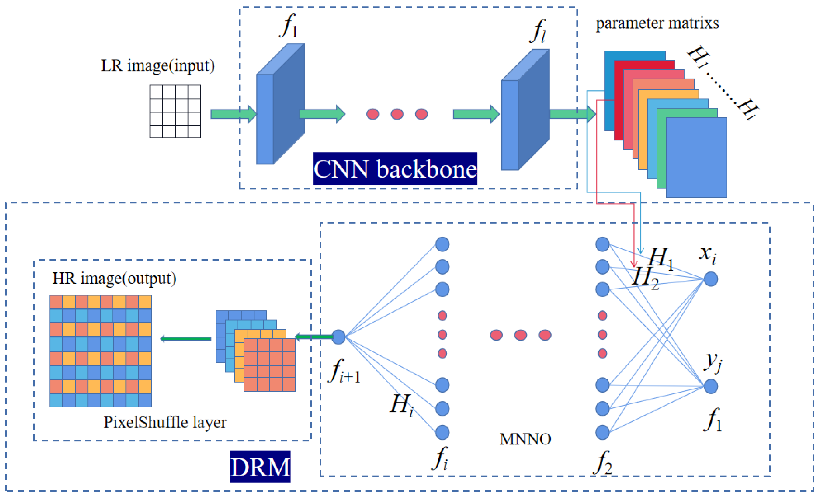
Unlike traditional CNN-based SISR methods that directly output the reconstructed HR pixels, we adopt a CNN backbone to estimate the parameters of the MNNO for each pixel.

2.3. Sampling Matrix

As argued in the previous subsection, the neighborhood of each pixel is only supposed to cover the corresponding sub-pixels in the HR image. It is clear that given a random float upsampling factor, the sub-pixels’ relative position in a local patch are probably different from other patches. However, for integer upsampling factors, the situations will be much simpler. Given a integer upsampling factor s, one LR pixel can be uniformly divided into s 2 sub-pixels. Assuming the origin is at the LR pixel, the relative coordinates of the sub-pixel at the i-th column and j-th row can be easily calculated by the symmetry principle as:
( x i ^ , y j ^ ) = ( 2 i s 1 2 s , 2 j s 1 2 s )
where ( x i ^ , y j ^ ) denotes the relative coordinates. Then, we can obtain an s 2 × 2 -sized coordinate matrix for each LR pixel.

2.4. Overview of the Architecture

Figure 3 illustrates the architecture of the proposed LDRN. The proposed method consists of two parts: the CNN backbone and the distribution reconstruction module (DRM). The CNN backbone is supposed to estimate the parameters for constructing the local distributions. The DRM then reconstructs the sub-pixels using Equations (3) and (5) and finally outputs the HR image via the pixel shuffle operation.
The recurrent-like architectures [37,38,39] are widely adopted by SISR methods to formulate the backbone. Though they exhibit outstanding performance, they clearly suffer from the expensive computation cost resulting from the multiple residual convolution blocks. For instance, typical light recurrent networks such as EDSR-baseline [40], SRResnet [41], etc., obtain over millions of parameters and take over 2.8 trillion Flops to process a 1920 × 1080 -sized image. Even the much more efficient VDSR [42] is also too large to be implemented on the hardware platforms [30]. To achieve extreme efficiency, we only adopt a few convolution layers to construct the baseline. Assuming the CNN backbone is formulated by L convolution layers, these L convolution layers are sequentially stacked. For the l-th layer, f l and f l + 1 are recorded as its input and output. Then, the process of the l-th layer can be expressed as:
f l + 1 = CN f l , W l , B l = σ 0 , W l f l + B l l < L W l f l + B l l = L
where W l and B l denote the convolution kernel and bias of the i-th layer, and ‘∗’ denotes the convolution operation. As a 2D convolution kernel, the shape of W l can be written as c l 1 × c l × k l × k l , where c l denotes the channel size of the output of the l-th layer and k l denotes the size of square kernel.
The DRM is supposed to conduct MNNO to obtain the final sub-pixels for each LR pixel via the sampling matrix and the parameters estimated by the CNN backbone. Then, these sub-pixels are re-arranged by the shuffling operation to reconstruct the final HR image. As described in Equation (5), using a larger N and larger n i to formulate the MNNO could help to approach a more complex and non-linear distribution. However, this will also introduce too high of a computation cost and make the algorithm quite inefficient. Moreover, the vanishing gradient is another serious challenge for a deep full connection neural network. To solve these two problems, we adopt a shallow and small-scale MNNO to formulate the DRM. First, the small-scale MNNO could save lots of parameters and computation. Second, the shallow depth could ensure back-propagating the gradient to the shallow layers of the CNN backbone and avoid the vanishing gradient.

2.5. Implementation Details

The proposed LDRN consists of a CNN backbone and DRM. For the CNN backbone, we set L = 4 , k 1 , c 1 = 5 , 64 , k 2 , c 2 = 3 , 32 , k 3 , c 3 = 3 , 32 , k 4 , c 4 = 3 , T M N N O { n 1 , n 2 , , n N } . To keep the size of the input LR image unchanged, we set the padding size of the l-th layer to k l 1 2 . As described in Section 2.4, we adopt shallow and small-scale settings for the DRM, so we set N = 2 and { n 1 , n 2 } = { 12 , 1 } . Therefore, we can easily obtain that c 4 = 37 based on Equation (6). Moreover, we adopt PReLU as the activation function for the CNN backbone and ReLU as the activation function for the DRM. With the above settings, the proposed method has 40k parameters in total.
To train the proposed LDRN, we adopt the DIV2K [43] as the training dataset and Set5 [44] as the validation set. The LR images are generated using Bicubic interpolation. The 32 × 32 pixel I L R patches are extracted from I L R sub-images, and 32 s × 32 s pixel I H R patches are extracted from I H R sub-images. The details of obtaining I L R and I H R will be extended in Section 3.1. We utilized random clipping to augment the training patches. Like previous studies, we transformed each patch into YCbCr space and only trained on the Y-channel. To train our model, we adopt Adam [45] as the optimizer and set the batchsize to 32. The learning rate is initialized to 10 3 . We test the PSNR performance on the validation set after the end of each training epoch. The learning rate will be halved when the PSNR performance on validation does not increase for 10 consecutive epochs. The minimum learning rate is set to 10 6 , and the maximum training epochs is set to 200. When the minimum learning rate is achieved or when the maximum training epoch is finished, the training will immediately stop. We choose the L1 loss as the loss function. The training takes roughly 90 min on a 2080Ti GPU. The PSNR is also used as the performance metric to evaluate our model. For each upscaling factor, we train a specific network. It is worth mentioning that because of the good Adam optimizer and the mature training strategy, the performance fluctuation of each method is less than 0.01 dB and hardly affects the comparison results. Therefore, we will not report the confidence intervals of the results in the following experiments.

3. Experiments

In this section, we evaluate the performance of the proposed method using five benchmark datasets. First, we describe the five benchmark datasets in detail. Then, we demonstrate the effectiveness of the proposed CNN backbone and DRM. Moreover, we also show that the settings given in Section 2.5 are the most appropriate settings for the proposed method. Finally, we compare the proposed method with several extremely efficient SISR methods to demonstrate the superiority of the proposed method.

3.1. Datasets

To train the proposed method, we adopt a training set from the DIV2K dataset as the training dataset, which contains 800 HR images with 2K resolution. To obtain the LR images, we downsample the HR images using bicubic kernels with a scale factor of s { 2 , 3 , 4 } . We group the I H R into 192 × 192 -sized patches with a stride of 192 and crop I L R patches to the size of 192 s × 192 s from the corresponding LR image with a stride of 192 s . In this way, we obtain 55510 non-overlapped training data pairs in total. In the testing stage, we introduced five widely used public datasets, including the Set5, Set14 [46], B100 [47], Urban100 [48] and Manga109 [49], to evaluate the performance of the proposed method and compared methods.

3.2. Ablation Investigation

In this subsection, we demonstrate the contribution of the proposed components, including the CNN backbone and the distribution reconstruction module, in detail.

3.2.1. CNN Backbone

We first compare the performance of the proposed CNN backbone with several existing backbones adopted by extremely efficient SISR methods, including SRCNN [11], ESPCN [19] and FSRCNN [50].
As shown in Table 1, the proposed backbone clearly surpasses existing backbones for all datasets. Especially on the most challenging datasets Manga109 and Urban100, the proposed backbone beats the second-best FSRCNN backbone by over 0.1 dB. The SRCNN’s backbone introducing large-sized convolution kernel does not provide positive effects for local distribution learning. Though FSRCNN’s backbone obtains the least parameters, it suffers from the poor receptive field of the 1 × 1 -sized convolution kernel, which cannot provide much information to support reconstructing the local distribution.

3.2.2. Distribution Reconstruction Module

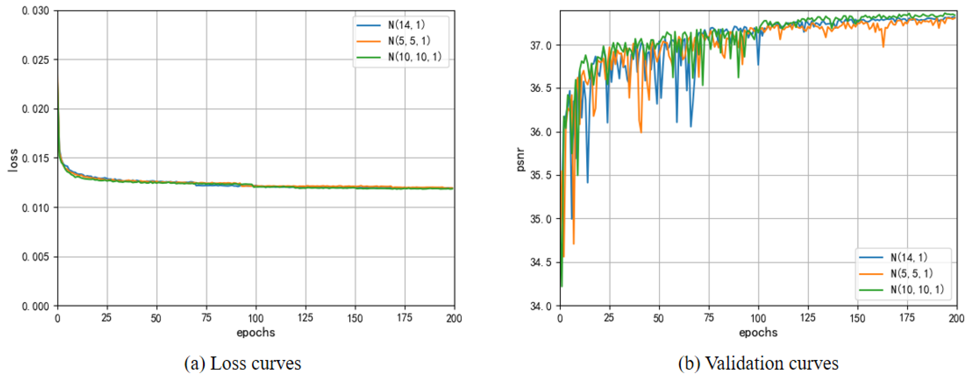
The distribution reconstruction module (DRM) is the core module in achieving the super resolution. As argued in Section 2.4, a deeper neural network in MNNO would suffer from gradient back-propagation and cannot achieve a better performance. We show the training loss curves and validation PSNR curves using N = { 12 , 1 } , N = { 5 , 5 , 1 } and N = { 10 , 10 , 1 } settings in Figure 4. The N = { 5 , 5 , 1 } setting obtains a closed number of parameters to N = { 12 , 1 } . Comparing the curves of N = { 12 , 1 } and N = { 5 , 5 , 1 } , using a similar scale of parameters to construct a deeper neural network cannot achieve a better performance. Moreover, from the results of N = { 10 , 10 , 1 } , using much more parameters to construct a deeper neural network also provides little help in improving the performance. Therefore, we adopt a two-layer neural network in MNNO to formulate the DRM.
Then, we investigate the best settings for a two-layer neural network. We construct a group of models with different MNNO settings thatinclude N = 0 , N = { 4 , 1 } , N = { 6 , 1 } , …, N = { 20 , 1 } , where N = 0 denotes the model using only a convolution layer rather than MNNO to output sub-pixels. From the results shown in Table 2, using small-scale settings to construct MNNO shows closed performances to a normal convolution layer. However, the larger MNNO does not always lead to a better performance. The larger MNNO leads to a more complex distribution model, which certainly increases the difficulty of estimating the MNNO parameters. Observing that the setting N = { 12 , 1 } achieves the best balance between complexity and performance, we adopt N = { 12 , 1 } setting to formulate the DRM.

3.3. Comparison with State-of-the-Art Methods

To fairly evaluate the performance of the proposed method, we compare the method with three typical, extremely efficient SISR methods, including SRCNN, FSRCNN and ESPCN, and another two recently proposed methods—HFSR [30] and TSSRN [29]. We retrained all compared methods using the same training strategy to ensure fair comparisons. Because HFSR [30] could only be applied on a × 2 scale, we only train the HFSR for a × 2 scale comparison.
For an objective evaluation, we calculate the PSNR and SSIM for different upscaling factors on five benchmark datasets. The quantitative results are shown in Table 3. The proposed method outperforms both × 2 (0.244 dB higher than the second average) and × 3 (0.106 dB higher than the second best) on five benchmark datasets of all compared methods. Although the proposed method is not the best in terms of × 4 (lower than the first average by 0.032 dB), the gap is very small and does not exceed 0.04 dB on average. To further illustrate the effects of different downsampling methods, we conduct an additional experiment by producing the LR images with Gaussian downsampling. Specifically, the Gaussian downsapling firstly blurs the HR image with a 3 × 3 Gaussian blur kernel and then downsamples the blurred image with a mean filter. Table 4 shows the comparison result. Comparing the bicubic results shown in Table 3 and Table 4, the Gaussian downsampling produces more serious LR degradation. Obviously, TSSRN obtains relatively good results for bicubic downsampling degradation and exhibits poor performance on the Gaussian downsampling degradation. By contrast, our LDRN achieves even greater performance gain from the bicubic interpolation. This observation certainly demonstrates that the proposed distribution learning architecture is robust to tougher situations.
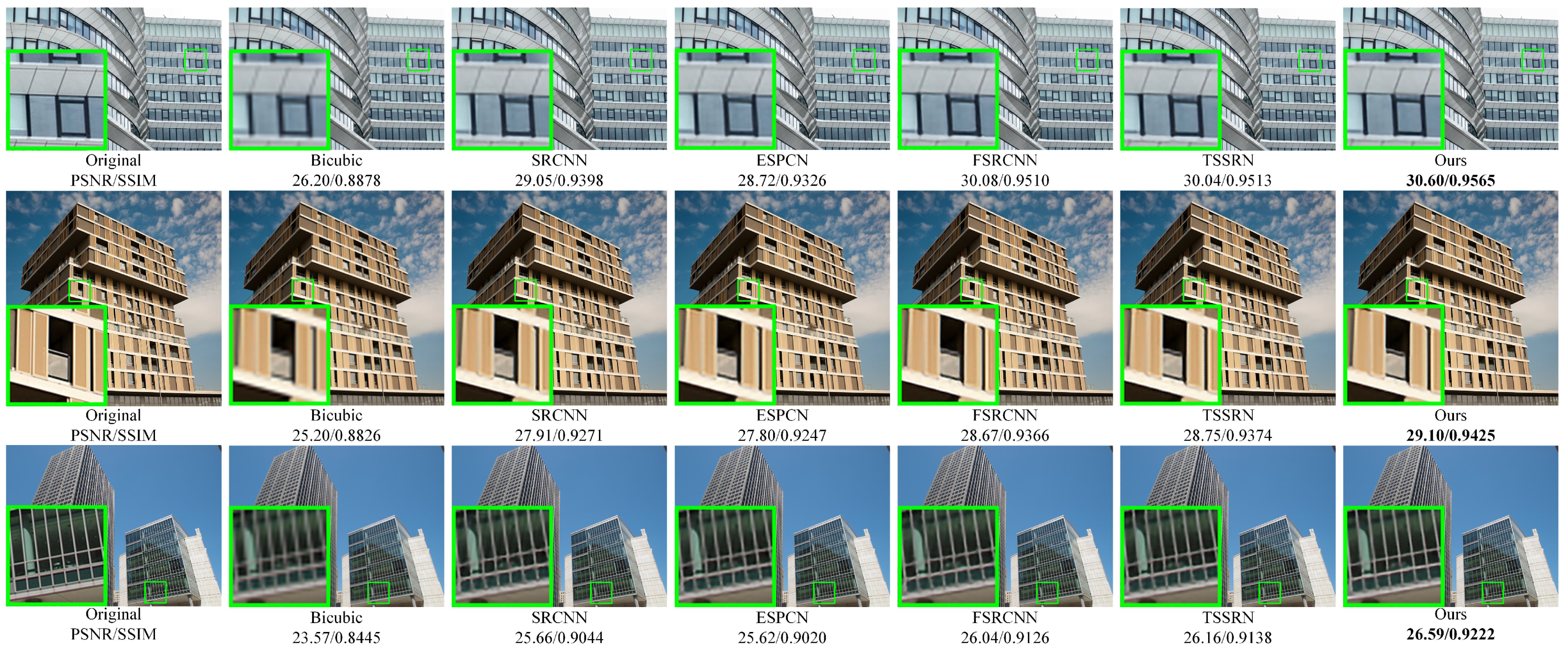
Moreover, we also provide the results of the subjective evaluation for the more challenging × 3 and × 4 scales, respectively, in Figure 5 and Figure 6. Because the HFSR can only process × 2 scaled images, it will not be included in this comparison. In the more challenging Urban100 and Manga109 datasets, our LDRN exhibits better detailed reconstruction ability caused by the MNNO.
To fully investigate the efficiency of all compared methods, we list the running times, parameters, FLOPs and memory costs of all compared methods for processing a 1920 × 1080 -sized image on the RTX 2080Ti GPU in Table 5. We also include typical efficient SISR methods VDSR [42] and EDSR [40] as references in the comparison. Compared to other methods, these two efficient methods have unaffordable computation and memory costs—VDSR requires 9.3 GB memory, and EDSR takes over 2.8T FLOPs and 244 ms to process a 1920 × 1080 sized images. As far as we know, other efficient SISR methods [24,25,52] (also called as lightweight methods) always achieve similar efficiencies between EDSR and VDSR. In contrast, the other methods contain less than 50k parameters and consume less than 3 GB memory for the same processing except for SRCNN. Accordingly, we can conclude the extreme efficiencies of these methods. Our method has a close running speed to HFSR and close memory cost to ESPCN, which certainly satisfies real-time processing. However, our LDRN contains the most parameters and the second most flops among these extremely efficient methods due to the MNNO.

4. Conclusions

In this paper, we propose a novel local distribution reconstruction network for extremely efficient single-image super-resolution. The proposed method consists of a CNN backbone and a distribution reconstruction module. To achieve extreme efficiency, we adopt a four-layer CNN to formulate the backbone. In the distribution reconstruction module, we propose a multi-layer neural network operator to approach the distribution model of the real scene and calculate the HR pixels by sampling. The ablation study demonstrates the effectiveness of the proposed CNN backbone and MNNO. The experiments on two downsampling methods show that the proposed method exhibits the ability to solve different kinds of LR degradation and clearly beats the second-best method with large margins (over 0.244 dB for × 2 in average) for more challenging Gaussian downsampling. Overall, the proposed method presents good performance and efficiency and shows a promising performance when deployed on hardware platforms.

Author Contributions

Conceptualization, W.W. and B.Z.; methodology, W.W. and B.Z.; software, W.X.; validation, W.W. and B.Z.; formal analysis, W.W. and A.H.; investigation, W.W., W.X. and A.H.; resources, W.W. and W.X.; data curation, W.X.; writing—original draft preparation, W.W., W.X. and B.Z.; writing—review and editing, B.Z.; visualization, W.X.; supervision, C.Y.; project administration, W.W. and B.Z.; funding acquisition, W.W. and B.Z. All authors have read and agreed to the published version of the manuscript.

Funding

This research is funded by National Nature Science Foundation of China (61501154, 62001146), and the APC is funded by National Nature Science Foundation of China (61501154).

Institutional Review Board Statement

Our study does not require ethical approval.

Informed Consent Statement

Our study does not involve humans.

Data Availability Statement

The research project will be available at https://github.com/XuWen6666/LDRN (accessed on 11 March 2022).

Conflicts of Interest

The authors declare that there is no conflict of interest exists in this research.

References

  1. Zhou, F.; Yang, W.; Liao, Q. Interpolation-based image super-resolution using multisurface fitting. IEEE Trans. Image Process. 2012, 21, 3312–3318. [Google Scholar] [CrossRef]
  2. Gilman, A.; Bailey, D.G.; Marsland, S.R. Interpolation models for image super-resolution. In Proceedings of the 4th IEEE International Symposium on Electronic Design, Test and Applications (Delta 2008), Hong Kong, China, 23–25 January 2008; pp. 55–60. [Google Scholar]
  3. Mallat, S.; Yu, G. Super-resolution with sparse mixing estimators. IEEE Trans. Image Process. 2010, 19, 2889–2900. [Google Scholar] [CrossRef] [Green Version]
  4. Chappalli, M.B.; Bose, N.K. Simultaneous noise filtering and super-resolution with second-generation wavelets. IEEE Signal Process. Lett. 2005, 12, 772–775. [Google Scholar] [CrossRef]
  5. Lo, K.H.; Wang, Y.C.F.; Hua, K.L. Joint trilateral filtering for depth map super-resolution. In Proceedings of the 2013 Visual Communications and Image Processing (VCIP), Kuching, Malaysia, 17–20 November 2013; pp. 1–6. [Google Scholar]
  6. Mei, Y.; Fan, Y.; Zhou, Y. Image super-resolution with non-local sparse attention. In Proceedings of the IEEE/CVF Conference on Computer Vision and Pattern Recognition, Nashville, TN, USA, 20–25 June 2021; pp. 3517–3526. [Google Scholar]
  7. Bendory, T.; Dekel, S.; Feuer, A. Super-resolution on the sphere using convex optimization. IEEE Trans. Signal Process. 2015, 63, 2253–2262. [Google Scholar] [CrossRef] [Green Version]
  8. Ng, M.K.; Bose, N.K. Mathematical analysis of super-resolution methodology. IEEE Signal Process. Mag. 2003, 20, 62–74. [Google Scholar] [CrossRef]
  9. Sun, L.; Hays, J. Super-resolution from internet-scale scene matching. In Proceedings of the 2012 IEEE International Conference on Computational Photography (ICCP), Seattle, WA, USA, 28–29 April 2012; pp. 1–12. [Google Scholar]
  10. Qu, Y.Y.; Liao, M.J.; Zhou, Y.W.; Fang, T.Z.; Lin, L.; Zhang, H.Y. Image super-resolution based on data-driven Gaussian process regression. In International Conference on Intelligent Science and Big Data Engineering; Springer: Berlin, Germany, 2013; pp. 513–520. [Google Scholar]
  11. Dong, C.; Loy, C.C.; He, K.; Tang, X. Learning a deep convolutional network for image super-resolution. In Proceedings of the ECCV, Zurich, Switzerland, 6–12 September 2014. [Google Scholar]
  12. Yang, S.; Wang, M.; Chen, Y.; Sun, Y. Single-image super-resolution reconstruction via learned geometric dictionaries and clustered sparse coding. IEEE Trans. Image Process. 2012, 21, 4016–4028. [Google Scholar] [CrossRef]
  13. Gu, S.; Zuo, W.; Xie, Q.; Meng, D.; Feng, X.; Zhang, L. Convolutional sparse coding for image super-resolution. In Proceedings of the IEEE International Conference on Computer Vision, Santiago, Chile, 7–13 December 2015; pp. 1823–1831. [Google Scholar]
  14. Wang, Z.; Liu, D.; Yang, J.; Han, W.; Huang, T. Deep Networks for Image Super-Resolution with Sparse Prior. In Proceedings of the ICCV, Santiago, Chile, 7–13 December 2015; pp. 370–378. [Google Scholar] [CrossRef] [Green Version]
  15. Yamashita, R.; Nishio, M.; Do, R.K.G.; Togashi, K. Convolutional neural networks: An overview and application in radiology. Insights Into Imaging 2018, 9, 611–629. [Google Scholar] [CrossRef] [Green Version]
  16. Yang, X.; Mei, H.; Zhang, J.; Xu, K.; Yin, B.; Zhang, Q.; Wei, X. DRFN: Deep recurrent fusion network for single-image super-resolution with large factors. IEEE Trans. Multimed. 2018, 21, 328–337. [Google Scholar] [CrossRef] [Green Version]
  17. Hui, Z.; Wang, X.; Gao, X. Two-stage convolutional network for image super-resolution. In Proceedings of the 2018 24th International Conference on Pattern Recognition (ICPR), IEEE, Beijing, China, 20–24 August 2018; pp. 2670–2675. [Google Scholar]
  18. Ronneberger, O.; Fischer, P.; Brox, T. U-Net: Convolutional Networks for Biomedical Image Segmentation. In Proceedings of the International Conference on Medical Image Computing and Computer-assisted Intervention, Munich, Germany, 5–9 October 2015. [Google Scholar]
  19. Shi, W.; Caballero, J.; Huszar, F.; Totz, J.; Aitken, A.P.; Bishop, R.; Rueckert, D.; Wang, Z. Real-Time Single Image and Video Super-Resolution Using an Efficient Sub-Pixel Convolutional Neural Network. In Proceedings of the CVPR, IEEE, Las Vegas, NV, USA, 27–30 June 2016. [Google Scholar] [CrossRef] [Green Version]
  20. Arirangan, S.; Kottursamy, K. Multi-scaled feature fusion enabled convolutional neural network for predicting fibrous dysplasia bone disorder. Expert Syst. 2021, e12882. [Google Scholar] [CrossRef]
  21. Saranya, A.; Kottursamy, K.; AlZubi, A.A.; Bashir, A.K. Analyzing fibrous tissue pattern in fibrous dysplasia bone images using deep R-CNN networks for segmentation. Soft Comput. 2021, 1–15. [Google Scholar] [CrossRef]
  22. Lan, R.; Sun, L.; Liu, Z.; Lu, H.; Pang, C.; Luo, X. MADNet: A fast and lightweight network for single-image super resolution. IEEE Trans. Cybern. 2020, 51, 1443–1453. [Google Scholar] [CrossRef]
  23. Chudasama, V.; Prajapati, K.; Upla, K. Computationally efficient super-resolution approach for real-world images. In Proceedings of the National Conference on Computer Vision, Pattern Recognition, Image Processing, and Graphics, Hubballi, India, 22–24 December 2019; Springer: Berlin, Germany, 2019; pp. 143–153. [Google Scholar]
  24. Liu, J.; Zhang, W.; Tang, Y.; Tang, J.; Wu, G. Residual feature aggregation network for image super-resolution. In Proceedings of the IEEE/CVF Conference on Computer Vision and Pattern Recognition, Seattle, WA, USA, 13–19 June 2020; pp. 2359–2368. [Google Scholar]
  25. Zhang, Y.; Wei, D.; Qin, C.; Wang, H.; Pfister, H.; Fu, Y. Context reasoning attention network for image super-resolution. In Proceedings of the IEEE/CVF International Conference on Computer Vision, Montreal, QC, Canada, 10–17 October 2021; pp. 4278–4287. [Google Scholar]
  26. Zhang, K.; Gool, L.V.; Timofte, R. Deep unfolding network for image super-resolution. In Proceedings of the IEEE/CVF Conference on Computer Vision and Pattern Recognition, Seattle, WA, USA, 13–19 June 2020; pp. 3217–3226. [Google Scholar]
  27. Prajapati, K.; Chudasama, V.; Patel, H.; Upla, K.; Raja, K.; Ramachandra, R.; Busch, C. Direct Unsupervised Super-Resolution Using Generative Adversarial Network (DUS-GAN) for Real-World Data. IEEE Trans. Image Process. 2021, 30, 8251–8264. [Google Scholar] [CrossRef]
  28. Prajapati, K.; Chudasama, V.; Patel, H.; Upla, K.; Raja, K.; Ramachandra, R.; Busch, C. Unsupervised Real-World Super-resolution Using Variational Auto-encoder and Generative Adversarial Network. In Proceedings of the International Conference on Pattern Recognition, Virtual, 4–6 February 2021; Springer: Berlin, Germany, 2021; pp. 703–718. [Google Scholar]
  29. Lee, J.; Lee, J.; Yoo, H.J. SRNPU: An Energy-Efficient CNN-Based Super-Resolution Processor With Tile-Based Selective Super-Resolution in Mobile Devices. IEEE J. Emerg. Sel. Top. Circuits Syst. 2020, 10, 320–334. [Google Scholar] [CrossRef]
  30. Kim, Y.; Choi, J.S.; Kim, M. A Real-Time Convolutional Neural Network for Super-Resolution on FPGA With Applications to 4K UHD 60 fps Video Services. IEEE Trans. Circuits Syst. Video Technol. 2019, 29, 2521–2534. [Google Scholar] [CrossRef]
  31. Dabov, K.; Foi, A.; Katkovnik, V.; Egiazarian, K. Image Denoising by Sparse 3-D Transform-Domain Collaborative Filtering. IEEE Trans. Image Process. 2007, 16, 2080–2095. [Google Scholar] [CrossRef]
  32. Zheng, B.; Chen, Y.; Tian, X.; Zhou, F.; Liu, X. Implicit dual-domain convolutional network for robust color image compression artifact reduction. IEEE Trans. Circuits Syst. Video Technol. 2019, 30, 3982–3994. [Google Scholar] [CrossRef]
  33. Zheng, B.; Yuan, S.; Slabaugh, G.; Leonardis, A. Image demoireing with learnable bandpass filters. In Proceedings of the IEEE/CVF Conference on Computer Vision and Pattern Recognition, Seattle, WA, USA, 13–19 June 2020; pp. 3636–3645. [Google Scholar]
  34. Zhou, X.; Fang, H.; Liu, Z.; Zheng, B.; Sun, Y.; Zhang, J.; Yan, C. Dense Attention-guided Cascaded Network for Salient Object Detection of Strip Steel Surface Defects. IEEE Trans. Instrum. Meas. 2021, 71, 5004914. [Google Scholar] [CrossRef]
  35. Zheng, B.; Yuan, S.; Yan, C.; Tian, X.; Zhang, J.; Sun, Y.; Liu, L.; Leonardis, A.; Slabaugh, G. Learning Frequency Domain Priors for Image Demoireing. IEEE Trans. Pattern Anal. Mach. Intell. 2021. [Google Scholar] [CrossRef]
  36. Zhao, H.; Zheng, B.; Yuan, S.; Zhang, H.; Yan, C.; Li, L.; Slabaugh, G. CBREN: Convolutional Neural Networks for Constant Bit Rate Video Quality Enhancement. IEEE Trans. Circuits Syst. Video Technol. 2021. [Google Scholar] [CrossRef]
  37. Zheng, B.; Tian, X.; Chen, Y.; Jiang, R.; Liu, X. Build receptive pyramid for efficient color image compression artifact reduction. J. Electron. Imaging 2020, 29, 033009. [Google Scholar] [CrossRef]
  38. Zheng, B.; Sun, R.; Tian, X.; Chen, Y. S-Net: A scalable convolutional neural network for JPEG compression artifact reduction. J. Electron. Imaging 2018, 27, 1. [Google Scholar] [CrossRef] [Green Version]
  39. Tian, X.; Zheng, B.; Li, S.; Yan, C.; Zhang, J.; Sun, Y.; Shen, T.; Xiao, M. Hard parameter sharing for compressing dense-connection-based image restoration network. J. Electron. Imaging 2021, 30, 053025. [Google Scholar] [CrossRef]
  40. Lim, B.; Son, S.; Kim, H.; Nah, S.; Mu Lee, K. Enhanced deep residual networks for single image super-resolution. In Proceedings of the CVPRW, Honolulu, HI, USA, 21–26 July 2017. [Google Scholar]
  41. Wang, X.; Yu, K.; Wu, S.; Gu, J.; Liu, Y.; Dong, C.; Qiao, Y.; Change Loy, C. Esrgan: Enhanced super-resolution generative adversarial networks. In Proceedings of the ECCV, Munich, Germany, 8–14 September 2018. [Google Scholar]
  42. Kim, J.; Kwon Lee, J.; Mu Lee, K. Accurate image super-resolution using very deep convolutional networks. In Proceedings of the CVPR, Las Vegas, NV, USA, 27–30 June 2016. [Google Scholar]
  43. Timofte, R.; Agustsson, E.; Gool, L.V.; Yang, M.H.; Zhang, L.; Lim, B.; Son, S.; Kim, H.; Nah, S.; Lee, K.M.; et al. NTIRE 2017 Challenge on Single Image Super-Resolution: Methods and Results. In Proceedings of the 2017 IEEE Conference on Computer Vision and Pattern Recognition Workshops (CVPRW), Honolulu, HI, USA, 21–26 July 2017. [Google Scholar] [CrossRef]
  44. Bevilacqua, M.; Roumy, A.; Guillemot, C.; Alberi-Morel, M.L. Low-complexity single-image super-resolution based on nonnegative neighbor embedding. In Proceedings of the British Machine Vision Conference 2012, Surrey, UK, 3–7 September 2012; pp. 1–135. [Google Scholar]
  45. Kingma, D.; Ba, J. Adam: A Method for Stochastic Optimization. In Proceedings of the ICLR, Banff, AB, Canada, 14–16 April 2014. [Google Scholar]
  46. Yang, J.; Wright, J.; Huang, T.S.; Ma, Y. Image super-resolution via sparse representation. IEEE Trans. Image Process. 2010, 19, 2861–2873. [Google Scholar] [CrossRef] [PubMed]
  47. Arbelaez, P.; Maire, M.; Fowlkes, C.; Malik, J. Contour detection and hierarchical image segmentation. IEEE Trans. Pattern Anal. Mach. Intell. 2010, 33, 898–916. [Google Scholar] [CrossRef] [PubMed] [Green Version]
  48. Huang, J.B.; Singh, A.; Ahuja, N. Single image super-resolution from transformed self-exemplars. In Proceedings of the IEEE Conference on Computer Vision and Pattern Recognition, San Diego, CA, USA, 20–25 June 2005; pp. 5197–5206. [Google Scholar]
  49. Matsui, Y.; Ito, K.; Aramaki, Y.; Fujimoto, A.; Ogawa, T.; Yamasaki, T.; Aizawa, K. Sketch-based manga retrieval using manga109 dataset. Multimed. Tools Appl. 2017, 76, 21811–21838. [Google Scholar] [CrossRef] [Green Version]
  50. Dong, C.; Loy, C.C.; Tang, X. Accelerating the Super-Resolution Convolutional Neural Network. In Proceedings of the Computer Vision–ECCV 2016, Amsterdam, The Netherlands, 11–14 October 2016; Leibe, B., Matas, J., Sebe, N., Welling, M., Eds.; Springer International Publishing: Cham, Switzerland, 2016; pp. 391–407. [Google Scholar]
  51. Wang, Z.; Bovik, A.; Sheikh, H.; Simoncelli, E. Image Quality Assessment: From Error Visibility to Structural Similarity. IEEE Trans. Image Process. 2004, 13, 600–612. [Google Scholar] [CrossRef] [Green Version]
  52. Hui, Z.; Gao, X.; Yang, Y.; Wang, X. Lightweight image super-resolution with information multi-distillation network. In Proceedings of the 27th Acm International Conference on Multimedia, Nice, France, 21–25 October 2019; pp. 2024–2032. [Google Scholar]
Figure 1. The local distribution of an LR pixel in situation. The green point denotes the pixel in the LR image, and the red point denotes the corresponding sub-pixels in the HR image.
Electronics 11 01348 g001
Figure 2. The proposed multi-layer neural network operator (MNNO) takes two-dimensional sampling coordinate points as input and outputs sampling values.
Electronics 11 01348 g002
Figure 3. The proposed LDRN consists of the CNN backbone and the DRM. The CNN backbone is used to generate the parameter matrix, and the DRM is used to generate the HR image.
Electronics 11 01348 g003
Figure 4. Training curves for N = (12,1), N = (5,5,1) and N = (10,10,1).
Electronics 11 01348 g004
Figure 5. The “052”, “087” and “096” images from the Urban100 dataset with an upscaling factor of 3.
Electronics 11 01348 g005
Figure 6. The “HighschoolKimengumi_vol20”, “AosugiruHaru” and “Nekodama” images from the Manga109 dataset with an upscaling factor of 4.
Electronics 11 01348 g006
Table 1. The comparison of PSNR and SSIM [51] with different CNN backbone settings on benchmark datasets. Bold indicates the best performance, while Underline indicates the second best.
DatasetScaleSRCNN BackboneFSRCNN BackboneESPCN BackboneOurs Backbone
Set5×2
×3
×4
37.10/0.9807
33.57/0.9647
30.59/0.9315
37.21/0.9809
33.80/0.9622
30.77/0.9343
36.62/0.9792
33.13/0.9612
30.19/0.9252
37.35/0.9812
33.81/0.9663
30.81/0.9349
Set14×2
×3
×4
32.63/0.9506
29.70/0.9104
27.44/0.8594
32.73/0.9509
29.86/0.9119
27.58/0.8619
32.33/0.9487
29.47/0.9069
27.21/0.8539
32.84/0.9514
29.88/0.9122
27.62/0.8626
B100×2
×3
×4
33.53/0.9534
28.99/0.8843
27.81/0.8478
33.41/0.9536
29.09/0.8856
27.89/0.8493
33.03/0.9512
28.76/0.8805
27.61/0.8429
33.49/0.9514
29.13/0.8863
27.93/0.8501
Urban100×2
×3
×4
30.00/0.9385
27.29/0.8914
24.51/0.8167
30.17/0.9397
27.51/0.8954
24.68/0.8220
29.34/0.9315
26.84/0.8827
24.22/0.8065
30.36/0.9417
27.61/0.8971
24.73/0.8239
Manga109×2
×3
×4
36.92/0.9864
31.03/0.9559
28.09/0.9199
37.20/0.9869
31.48/0.9591
28.45/0.9254
35.89/0.9839
30.16/0.9481
27.41/0.9090
37.45/0.9873
31.60/0.9601
28.57/0.9270
Table 2. The comparison of PSNR and SSIM of different N settings with upsampling factor 2 on benchmark datasets. Blod indicates the best performance, while Underline indicates the second best.
DatasetN = 0N = (4,1)N = (6,1)N = (8,1)N = (10,1)N = (12,1)N = (14,1)N = (16,1)N = (18,1)N = (20,1)
Set537.2637.2637.2837.3137.3437.3537.3537.3637.3437.35
Set1432.8032.8132.8132.8632.8632.8832.8432.8432.8832.83
B10033.4733.4633.4733.4933.5033.5133.4933.5033.5133.49
Urban10030.2330.2530.3130.3330.4030.4130.3630.4130.4330.36
Manga10937.2537.3637.3237.4037.4937.5037.4537.4437.4837.36
Table 3. The results of PSNR and SSIM on public benchmark datasets (Bicubic). Bold indicates the best performance, while Underline indicates the second best.
DatasetScaleBicubicSRCNN
ECCV’14
FSRCNN
ECCV’16
ESPCN
CVPR’16
HFSR
TCSVT’19
TSSRN
JETCAS’20
LDRN
Proposed
Set5×2
×3
×4
33.68/0.9644
30.90/0.9366
28.46/0.8918
36.83/0.9798
33.37/0.9633
30.45/0.9298
37.09/0.9806
33.78/0.9660
30.84/0.9350
36.82/0.9797
33.42/0.9632
30.48/0.9291
37.13/0.9807
-/-
-/-
37.18/0.9808
33.78/0.9662
30.87/0.9355
37.35/0.9812
33.86/0.9666
30.82/0.9349
Set14×2
×3
×4
30.23/0.9260
27.89/0.8785
25.99/0.8219
32.46/0.9495
29.60/0.9090
27.34/0.8573
32.68/0.9505
29.87/0.9117
27.61/0.8617
32.46/0.9494
29.65/0.9090
27.40/0.8578
32.67/0.9505
-/-
-/-
32.71/0.9507
29.84/0.9115
27.64/0.8624
32.88/0.9516
29.92/0.9125
27.61/0.8624
B100×2
×3
×4
30.95/0.9266
27.65/0.8520
26.70/0.8142
33.20/0.9522
28.91/0.8829
27.74/0.8453
33.34/0.9532
29.09/0.8854
27.92/0.8493
33.16/0.9519
28.89/0.8823
27.74/0.8459
33.36/0.9532
-/-
-/-
33.39/0.9535
29.08/0.8854
27.94/0.8497
33.51/0.9543
29.14/0.8865
27.92/0.8498
Urban100×2
×3
×4
26.89/0.8935
25.22/0.8406
23.17/0.7631
29.68/0.9355
27.20/0.8891
24.47/0.8140
29.95/0.9380
27.51/0.8944
24.69/0.8214
29.49/0.9332
27.08/0.8864
24.42/0.8124
29.97/0.9384
-/-
-/-
30.05/0.9391
27.51/0.8947
24.73/0.8223
30.41/0.9422
27.64/0.8978
24.73/0.8238
Manga109×2
×3
×4
31.27/0.9628
27.27/0.9123
25.30/0.8655
36.39/0.9851
30.78/0.9536
27.95/0.8173
37.02/0.9864
31.46/0.9585
28.50/0.9252
36.46/0.9850
30.71/0.9521
27.89/0.9158
37.05/0.9865
-/-
-/-
37.10/0.9866
31.49/0.9587
28.63/0.9266
37.50/0.9875
31.67/0.9604
28.57/0.9270
Table 4. The results of PSNR and SSIM on public benchmark datasets (Gaussian). Bold indicates the best performance, while Underline indicates the second best.
DatasetScaleBicubicSRCNNFSRCNNESPCNHFSRTSSRNLDRN
Set5×2
×3
×4
32.10/0.9517
30.27/0.9292
28.18/0.8884
36.71/0.9793
33.35/0.9633
30.39/09298
36.99/0.9803
33.64/0.9654
30.61/0.9330
36.64/0.9791
33.27/0.9624
30.27/0.9269
36.55/0.9788
-/-
-/-
35.57/0.9754
32.03/0.9518
29.82/0.9207
37.24/0.9809
33.69/0.9658
30.72/0.9345
Set14×2
×3
×4
29.02/0.9054
27.48/0.8696
25.50/0.8091
32.39/0.9489
29.50/0.9083
27.22/0.8561
32.59/0.9502
29.70/0.9101
27.37/0.8580
32.29/0.9486
29.52/0.9077
27.18/0.8543
32.12/0.9465
-/-
-/-
31.53/0.9428
28.72/0.8982
26.32/0.8369
32.85/0.9515
29.73/0.9109
27.45/0.8605
B100×2
×3
×4
29.73/0.9038
27.35/0.8429
26.56/0.8115
33.15/0.9519
28.85/0.8820
27.67/0.8453
33.33/0.9532
28.94/0.8832
27.73/0.8465
33.05/0.9511
28.74/0.8803
27.61/0.8442
32.80/0.9483
-/-
-/-
32.30/0.9451
28.22/0.8725
27.36/0.8395
33.48/0.9542
28.99/0.8847
27.82/0.8485
Urban100×2
×3
×4
25.87/0.8679
24.88/0.8303
23.04/0.7604
29.57/0.9341
27.15/0.8889
24.43/0.8154
29.95/0.9377
27.40/0.8929
24.59/0.8203
29.40/0.9319
26.98/0.8855
24.28/0.8103
29.35/0.9323
-/-
-/-
28.14/0.9187
25.93/0.8664
23.92/0.8010
30.37/0.9418
27.59/0.8978
24.71/0.8254
Manga109×2
×3
×4
29.38/0.9461
26.74/0.9045
23.14/0.8248
36.32/0.9846
30.74/0.9537
27.71/0.9156
37.09/0.9864
31.38/0.9582
28.21/0.9225
36.29/0.9845
30.58/0.9517
27.50/0.9120
36.31/0.9845
-/-
-/-
34.41/0.9790
28.55/0.9335
23.19/0.8430
37.43/0.9872
31.56/0.9600
28.32/0.9247
Table 5. The results of running time evaluation and parameters.
MethodSRCNNESPCNFSRCNNHFSRTSSRNVDSREDSRLDRN
Parameters57k21k13k20k14k680k1368k40k
Time (ms)0.910.490.811.020.601.64244.211.16
FLOPs475.1G44.1G54.4G41.5G44.7G6124.9G2839.3G83.1G
Memory (GB)5.22.62.92.12.39.37.22.6
Publisher’s Note: MDPI stays neutral with regard to jurisdictional claims in published maps and institutional affiliations.