Mode Switching Frequency of Electrohydraulic-Power-Coupled Electric Vehicles with Different Delay Control Times

Abstract

The variability of vehicle operating conditions and the multiplicity of coupler dynamics inevitably increase the frequency and complexity of cooperative power control. In this study, a novel electromechanical–hydraulic-power-coupled electric vehicle is developed and investigated. This vehicle integrates a conventional electric motor with a hydraulic pump/motor to interconvert electrical, mechanical, and hydraulic energies, while a rule-based dynamic optimal energy management strategy is designed to achieve dynamic switching of operating modes according to the operating conditions. Thus, the power-switching sensitivity is reduced by adding a delay determination link to the Stateflow. Results show that the addition of the delay link has a small effect on classical road conditions and significant suppression of road conditions with high-power-switching frequency. Therefore, the method proposed in this paper improves the energy efficiency, stability, and economic performance of electrohydraulic-power-coupled electric vehicles, which will hopefully provide a good reference for the development of electrohydraulic vehicles.

1. Introduction

1.1. Research Motivation

Since peak carbon occurred in the 1970s, carbon neutral national goals have been proposed, and the research and application of new energy vehicles is becoming increasingly more focused, but the development of electric vehicles is gradually encountering bottlenecks. Batteries must be improved in terms of size, cost, and capacity; conversely, the frequent start and stop of pure electric vehicles generate peak torque, creating load shocks and damaging the state of charge (SOC) of the battery, reducing its service life. Also, the use of braking energy recovered as electric energy in many working conditions of pure electric vehicles is low [1,2]. With high-power density; fast-energy charging and discharging; and high braking energy recovery rates, hydraulic systems are widely used in hybrid vehicles for auxiliary drive, to reduce peak motor power, and to improve vehicle dynamics [3,4,5]. However, most of the recent research on hydraulic hybrid electric vehicles has been to add a hydraulic auxiliary facility to the original pure electric vehicle, as the addition of a hydraulic system has a more obvious change to the starting acceleration characteristics of the electric vehicle. In addition, very little research has been done to couple the electric energy device with the hydraulic energy device to form a new device where the mechanical energy inside the new device can be the interconversion of electrical and hydraulic energy that replaces the original vehicle components. Additionally, the design and research of the control strategy is also the key to give full play to the advantages of electro-hydraulic vehicles. The logic threshold control strategy is a simple and effective control algorithm, but there is still little research on the logic threshold control strategy that focuses on the frequency of multi-mode switching in the vehicle under the control of the strategy.

1.2. Literature Review

Electric vehicles (EVs) and battery technology are gaining huge popularity, and the trend toward low-energy consumption, environmental pollution prevention, and other advantages of EVs has developed markedly. As an important component of on-board energy storage, battery technology strongly affects safety and economy; however, poor battery design, high battery maintenance costs, and abnormal battery failure make battery safety a potential problem [6,7,8]. Electrohydraulic-power-coupled high-performance electric vehicles have become an important research topic in the emerging field of energy vehicles because the HPC-EV design replaces the traditional drive motor, transmission, and auxiliary drive system of electric commercial vehicles. The organic combination of mechanical and electrohydraulic properties can effectively increase vehicle lifetime, and hydraulic power synergy can markedly reduce electric peak torque and allow a substantial increase in power for fast-starting vehicles. Researchers have investigated these topics in detail.

Table 1. Summary of the literature.

Researchers	Contribution	Year
Liu, H., Y. Jiang, and S. Li	Designed an electrohydrostatic hybrid power system, proposed a downhill speed control method	2019
Hu, J., B. Mei, H. Peng, and Z. Guo	Proposed a discrete speed ratio control strategy for the characteristics of a hydraulic system with high-energy loss	2019
Gong, J., D. Zhang, Y. Guo, C. Liu, Y. Zhao, P. Hu, and W. Quan	Proposed a new electrohydraulic system integrating recovery and regeneration devices	2019
Liu, H., G. Chen, C. Xie, D. Li, J. Wang, and S	Study of the energy-saving characteristics of electrohydrostatic hybrid railcars	2020
Yang, J., T. Zhang, H. Zhang, J. Hong, and Z. Meng	Start-up acceleration characteristics of a new power-coupled electric vehicle	2020
Yang, J., T. Zhang, J. Hong, H. Zhang, Q. Zhao, and Z. Meng	Proposed a new drive control strategy and fuzzy logic optimization study for electric vehicles	2021
Hong, J., F. Ma, and X. Xu	Characteristics of a new power-coupled electric vehicle considering different electrohydraulic distribution ratios	2021

details the research results produced by different researchers in related areas. Liu Huanlong et al. designed an electrohydrostatic hybrid power system. The energy-saving characteristics of the system’s hydraulic energy recovery and coupling were verified through simulation and indicated an energy recovery efficiency of up to 50%; the new coupling method can also markedly reduce power consumption. Concurrently, they designed an electrohydrostatic hybrid power system, proposed a downhill speed control method, and verified the effectiveness of the method through experiments [9,10]. Hu et al. proposed a discrete speed ratio control strategy for the characteristics of a hydraulic system with high-energy loss and used a genetic algorithm to optimize the discrete speed ratio. The proposed control strategy markedly reduced the energy loss of the hydraulic system [11]. Gong proposed a new electrohydraulic system integrating recovery and regeneration devices. A rule-based control strategy was used to achieve real-time control. Results showed that vehicles with this energy-saving system could reduce energy consumption by approximately 17.6% compared with ordinary vehicles [12]. Yang Jian and Meng Zewen et al. proposed a new electromechanical–hydraulic power-coupled drive system to simplify the layout of the pure electric vehicle drive system and improve vehicle acceleration and proposed a new electromechanical–hydraulic power-coupled drive system for the characteristics of high torque of the hydraulic drive system. They also proposed a method that combines real-time feedback of the accumulator output torque with PID control so that the feasibility and power performance of the system can be substantially improved by the feasibility and correctness of the system, which are verified by studying the starting acceleration characteristics and braking characteristics of the new electromechanical–hydraulic power-coupled electric vehicle [13,14,15]. By redesigning the drive control strategy and performing a fuzzy logic optimization study of the new electromechanical–hydraulic power-coupled electric vehicle, the energy utilization efficiency improved, and the driving range increased.

1.3. Challenges and Problems

First, the electromechanical–hydraulic-power-coupling device is currently in development and design stage due to the limitations of hybrid technology and theoretical research. There is no way to directly apply the device to the vehicle; only through simulations can we verify the rationality of the control strategy.

Second, the vehicle speed, SOC, and battery pressure have fast real-time response characteristics during operation, and hysteresis is inevitable.

Third, because the project is implemented in AMEsim and Simulink joint simulations, road information can only be used with some international standard road conditions and real measured road conditions as the formal road conditions of the vehicle.

1.4. Contributions of This Work

To address these issues, this study makes several notable contributions and improvements to the literature as follows:

A new electromechanical–hydraulic coupled power unit is proposed, which integrates a conventional electric motor with a piston pump/motor, allowing the interconversion of electrical, mechanical, and hydraulic energy.

Based on the new electromechanical–hydraulic-coupling power unit, a rule-based dynamic optimal energy management strategy is designed to switch the operating modes.

The incorporation of a delayed control link is proposed based on the switching frequency problem for the operating modes.

The effect of the inclusion of the delayed control link on the vehicle following speed, battery SOC, and mode-switching frequency under different road conditions is analysed.

1.5. Organization of the Paper

Section 2 primarily clarifies the structural principles of the electromechanical–hydraulic-power-coupled electric vehicle. Section 3 focuses on the selection of model parameters and the creation of the model, the construction of the control strategy, and the addition of the time-delay control strategy. Section 4 focuses on the analysis and discussion of the effects caused by the addition of the time-delay link under classical road conditions. Section 5 focuses on the validity of the delay control strategy through self-testing road conditions and the effect of different delay control times on the mode-switching frequency.

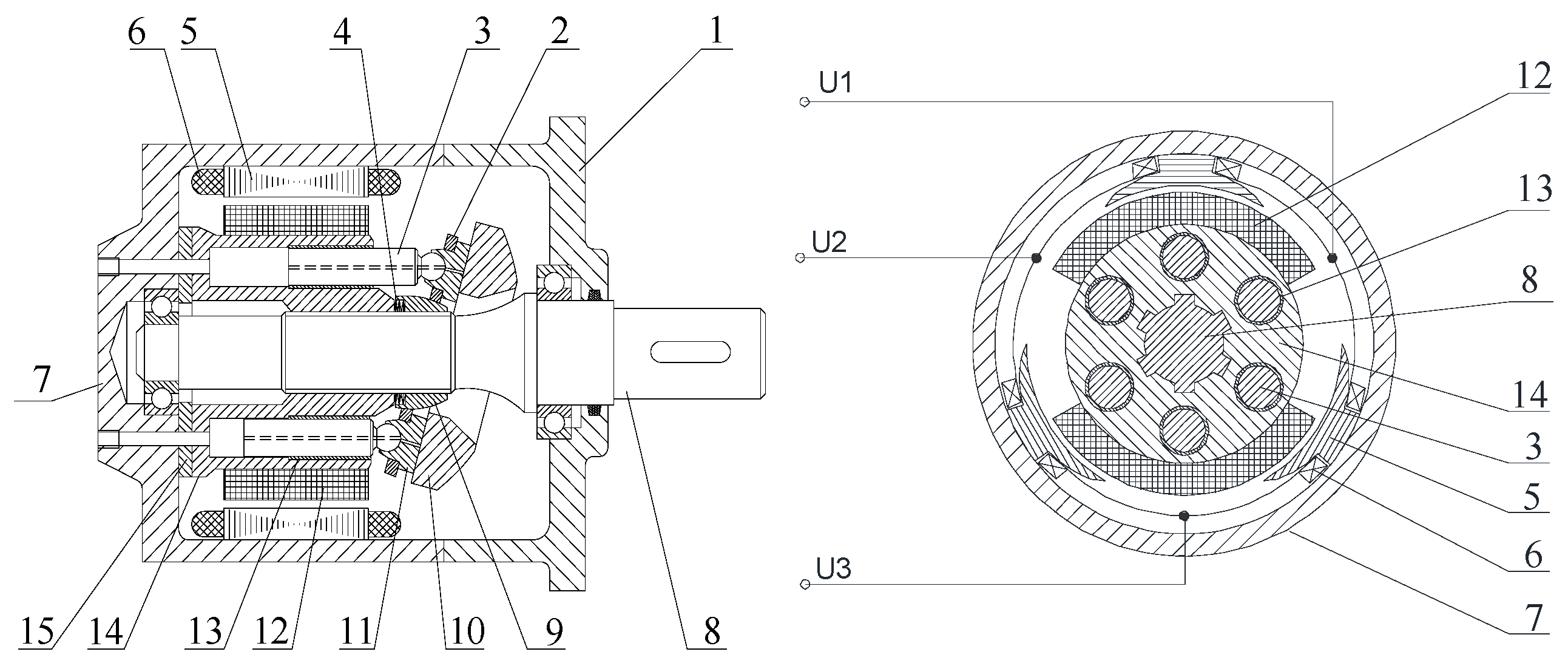
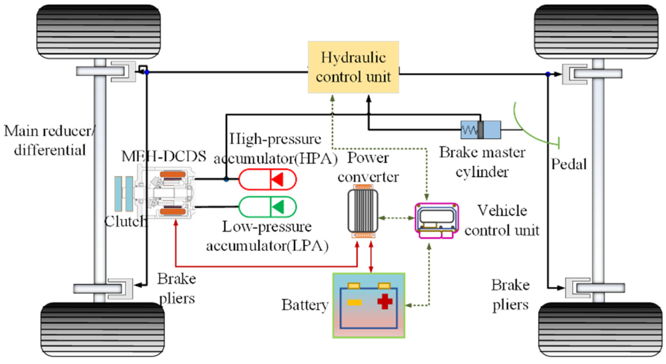
2. Structural Principle of an Electrohydraulic-Power-Coupled Electric Vehicle

The structure of the electrohydraulic coupler is shown in Figure 1 and can be described as a hydraulic energy device that consists of an electrical energy device composed of an external lead terminal, a stator core, a stator winding, a permanent magnet, a plunger, a valve plate, and other structures. This device mutually converts electric, mechanical, and hydraulic energies.

When the electrohydraulic coupler is used as a motor, the three-phase AC voltage is connected to the external lead terminal. The stator core and stator winding are affected by the energized current to form a composite electromagnetic field. The generated electromagnetic force drives the rotor and cylinder to rotate, thereby driving the drive shaft to output externally. Mechanical energy converts the electrical energy into mechanical energy. When used as a generator, the drive shaft is rotated by an external force, which in turn, drives the cylinder rotor to rotate and finally outputs electrical energy through the lead terminal, converting mechanical energy into electrical energy.

When the electrohydraulic coupler is used as a hydraulic pump, the rotating shaft is driven by electric power or external mechanical power, and then, the cylinder block and other components are driven to rotate. The plunger reciprocates under the action of the swashplate and moves to the right, changing the pump chamber’s volume. Hydraulic oil enters the pump cavity; the plunger moves to the left; the volume of the pump cavity decreases; the oil pressure rises; and high-pressure oil is output from the pump cavity through the valve plate. This reciprocal process transforms mechanical energy into hydraulic energy. As a hydraulic motor, the device inputs hydraulic power and outputs mechanical power, transforming hydraulic energy into mechanical energy.

The electrohydraulic coupler [16,17,18,19] is installed on the electric vehicle to create an electromechanical–hydraulic-power-coupled electric vehicle and primarily includes battery packs, high-voltage accumulators, low-voltage accumulators, electrohydraulic couplers, and primary reducer/differential components. The basic structure is shown in Figure 2. The only power source of electrohydraulic-power-coupled electric vehicles comes from the battery, and the hydraulic energy of the high-pressure accumulator comes from braking regeneration or conversion of electrical energy. During driving, hydraulic power is used to drive the vehicle independently or with auxiliary electric power when driving at low speed; electric power is primarily used to drive the vehicle when driving at high speed. During braking, when the initial braking speed is high, electric dynamic braking is used, and the inertial energy is recovered into the power battery in the form of electric energy; when the braking speed is low, hydraulic dynamic braking is used, and the inertial energy is in the form of hydraulic energy. Recycled to the high-pressure accumulator; when the braking intensity is high, hydraulic power and electric power will be used to brake concurrently, and the braking energy will be converted into electric and hydraulic energy and stored in the battery and high-pressure accumulator, respectively [20,21].

3. Model Building and Control Strategy Building

The power-matching models of electromechanical–hydraulic-power-coupled electric vehicles primarily include mechanical power (vehicle power), electric power, and hydraulic power models.

3.1. Vehicle Dynamic Model

When a car is running on a straight road, the total resistance, ΣF_t, generally consists of four parts: rolling resistance, F_f, gradient resistance, F_i, acceleration resistance, F_j, and air resistance, F_w. The balance equation of the car driving process is:

$$\{\begin{array}{l}{\displaystyle \sum F_t=F_f+F_i+F_j+F_w}\\ F_f=G\times f\\ F_i=mg\times sin\alpha \\ F_j=\delta m\frac{du}{dt}\\ F_w=\frac{C_{D}A{u}^2}{21.25}\end{array}$$

(1)

where G is the total gravity of the vehicle; u is the speed of the vehicle; f is the rolling resistance coefficient; m is the total mass of the vehicle; g is the acceleration of gravity; α is the gradient; δ is the rotation mass conversion coefficient; and C_D is the air resistance coefficient.

3.2. Electrodynamic Model

3.2.1. Motor Parameter Matching

Electromechanical–hydraulic-power-coupled electric vehicles are essentially pure electric vehicles [22,23,24]. Although there are hydraulic power forms in the power transmission, the parameters of the electric power must be matched and designed first, which directly affects the power and economy of the vehicle. The drive motor is a key component of an electrohydraulic hybrid vehicle, which not only needs to meet the operating requirements of the vehicle but also needs to adapt to the environmental changes in various driving conditions. It also needs to provide the driver with as much comfort as possible, which requires a high degree of smoothness in the operation of the drive motor, as well as a high torque at low speeds and a relatively wide range of constant power characteristics. Compared with motors such as DC motors, AC induction motors, stepper motors, switched reluctance motors, and permanent magnet synchronous motors have the advantages of good smoothness of operation, fast response, easy control, and small volume per unit of power, and in recent years, the research on permanent magnet synchronous motors has gradually matured [25,26] so the motor power system of this system uses permanent magnet synchronous motors [27].The power of the driving motor of an electric vehicle should be able to meet the requirements for maximum vehicle speed, acceleration time, and maximum gradeability. Therefore, the drive motor should meet the requirements of the three working conditions simultaneously:

$$P_{mmax}\ge max\left(P_1,P_2,P_3\right)$$

(2)

where P₁ [28,29] is the required power when the vehicle is climbing at a stable speed, and the acceleration resistance can be ignored; P₂ is the required power when the vehicle is traveling at the maximum speed evenly; P₃ is the power required during acceleration, and the gradient resistance is ignored during acceleration, which is primarily affected by air resistance, rolling resistance, and acceleration resistance:

$$\{\begin{array}{l}{P}_1=\frac{1}{{\eta }_T}\left(\frac{Gfcos\theta u_1}{3600}+\frac{Gsin\theta u_1}{3600}+\frac{C_{D}A{u}_1^3}{76140}\right)+P_{acc}\\ P_2=\frac{1}{{\eta }_T}\left(\frac{Gf{u}_{maxm}}{3600}+\frac{C_{D}A{u}_{maxm}^3}{76140}\right)+P_{acc}\\ P_3=\frac{1}{{\eta }_T}\left(\frac{Gf{u}_2}{5400}+\frac{\delta m{u}_2^2}{3600\times 7.2\times t}+\frac{C_{D}A{u}_2^3}{76140\times 2.5}\right)+P_{acc}\end{array}$$

(3)

where u_maxm is the highest vehicle speed in pure electric mode; u₁ is the required vehicle speed at the maximum climbing degree in pure electric mode; u₂ is the final acceleration speed when starting on the spot; Pacc is the total power consumed by the on-board accessories; η_T is the mechanical transmission efficiency; C_D is the drag coefficient; A is the windward area; G is the total weight of the vehicle; and δ is the rotational mass transfer coefficient; θ is the angle of the slope.

3.2.2. Battery Parameter Matching

It is necessary to consider the selection of battery peak power, P_maxb, while also satisfying factors such as maximum vehicle speed, equipment power consumption, and vehicle load [30]. According to the real situation and the matching result of the motor, the maximum design power of the battery pack is:

$$P_{maxb}=\frac{P_{max}}{{\eta }_b}$$

(4)

where η_b is the total efficiency of the battery pack. If a nickel-metal hydride battery is used as an energy storage element, according to the change curve of single internal resistance, the battery’s internal resistance is lower in the range of battery state of charge of 0.2 to 0.8, and the battery efficiency is higher at this time. This interval is beneficial to prolong the service life of the battery when η_b = 0.6. The total number of battery cells, n_bc, is:

$$\{\begin{array}{l}{P}_{maxb}{}_c=\frac{U_{bc}^2}{4\times R_{bc}}\\ n_{bc}=\frac{1000\times P_{maxb}}{P_{maxb}{}_c}\end{array}$$

(5)

where U_bc is the rated voltage of the single battery, and R_bc is the internal resistance of the single battery.

According to the calculation of the total number of batteries, n_bc = 219, according to the real situation and the arrangement of battery cells, n_bc = 240 is used in this study to facilitate the arrangement. The rated voltage of the available battery pack is:

$$U_b=n_{bc}\times U_{bc}$$

(6)

3.3. Hydraulic Power Model

Hydraulic power participates in both driving and regenerative braking, which is the unique feature of this power transmission system and plays an irreplaceable role in the smooth operation and transmission efficiency of the overall system [31]. It is necessary to calculate the maximum required power in each driving state first and then match the parameters of the hydraulic power and the hydraulic accumulator. The power consumed by the vehicle under accelerated driving conditions on a flat road is:

$$P_{max}=\frac{1}{{\eta }_T}\left(\frac{Gf{u}_3}{5400}+\frac{\delta m{u}_3^2}{3600\times 7.2\times t}+\frac{C_{D}A{u}_3^3}{76140\times 2.5}\right)+P_{acc}$$

(7)

where u₃ is the final acceleration speed in the hydraulic pump/motor single drive mode; η_h is the mechanical transmission efficiency from the hydraulic system to the wheels; and P_max is the maximum power required in the hydraulic pump/motor single drive mode.

The swashplate opening, β, and output torque, T_p, of the hydraulic pump/motor can be described as:

$$\{\begin{array}{l}-1\le \beta \le 1\\ T_p=\frac{\Delta p{V}_p\beta }{2\pi }\end{array}$$

(8)

where β is the opening of the swashplate [−1, 1], which corresponds to [−20°, 20°]; ∆p is the inlet and outlet pressure difference; and V_p is the displacement.

The formula for calculating the maximum torque, T, of hydraulic power is:

$$T=9549\times \frac{\partial \times P_{maxa}}{n_{maxa}}$$

(9)

where $\partial$ is the torque adaptability coefficient, and n_maxa is the maximum power speed.

The volume and initial pressure of a hydraulic accumulator determine how much energy it can absorb and how much energy it can provide as output; thus, the focus of the matching of hydraulic accumulators lies in the volume and initial pressure of the accumulator. The greater the volume and initial pressure of the hydraulic accumulator are, the stronger the hydraulic power system’s ability to provide torque and recover braking energy.

Accumulator Model

The accumulator model is designed according to the real working conditions, such as the size of the car space, the material of the hydraulic accumulator, the sealing capacity of the hydraulic accumulator, and the working pressure of the commonly used hydraulic equipment.

According to Boyle’s gas law:

$$p_0{V}_0^n=p_1{V}_1^n=p_2{V}_2^n$$

(10)

where p₀ is the charging pressure of the accumulator; V₀ is the charging volume of the accumulator and the total volume of the accumulator; p₁ is the lowest working pressure of the accumulator; V₁ is the gas volume when the pressure in the accumulator is p₁; p₂ is the highest working pressure of the accumulator; V₂ is the gas volume when the pressure of the accumulator is p₂; and n is a multivariable index, where n = 1 in an isothermal state, and n = 1.4 in an adiabatic state.

The calculation formula for the minimum working pressure, p₁, of the accumulator is:

$$p_1=\frac{2\mathsf{\pi }\left(Gf+\frac{C_{D}A{u}_{maxa}^2}{21.15}\right)}{V_{a}i}$$

(11)

where V_a is the displacement of the hydraulic pump/motor, i is the transmission ratio, and u_maxa is the highest vehicle speed in the hydraulic pump/motor single drive mode.

Assuming that the vehicle is driving on a straight road, the energy lost and recovered by the vehicle is:

$$\{\begin{array}{l}\frac{1}{2}\delta m\left(u_4{}^2-u_3{}^2\right)=E_1+E_2\\ E_1=mgfS+\frac{C_{D}A}{21.15}{\left(u_4-at\right)}^2\\ E_2=-{\displaystyle {\int }_{v1}^{v2}pdv=\frac{p_1{v}_1{}^{\mathrm{n}}}{n-1}\left(v_2^{1-n}-v_1{}^{1-n}\right)=\frac{p_1{v}_1}{n-1}\left[{\left(\frac{p_1}{p_2}\right)}^{\frac{1-n}{n}}-1\right]}\end{array}$$

(12)

where u₃ and u₄ are the speeds of the vehicle at t₃ and t_4, respectively; E₁ is the lost energy; E₂ is the recovered energy; δ is the conversion coefficient of the car’s rotating mass; S is the braking displacement of the vehicle; and a is the deceleration of the vehicle braking.

We now combine these formulae to obtain:

$$V_0=\frac{\left(n-1\right)\left[\frac{1}{2}\delta m\left(u_4^2-u_3^2\right)-\frac{C_{D}A}{21.15}{\left(u_4-at\right)}^2-GfS\right]}{p_1\left[{\left(\frac{p_1}{p_2}\right)}^{\frac{1-n}{n}}-1\right]}$$

(13)

The effective working volume, V_x, is the variability of the gas volume during the change from the lowest working pressure, P₁, to the highest working pressure, P₂, in the hydraulic accumulator:

$$V_x=\frac{V_0{\left(p_1/p_0\right)}^{-1/n}}{{\left(1-p_1/p_2\right)}^{-1/n}}$$

(14)

The basic parameters of the complete vehicle are shown in

Table 2. Basic parameters of the entire vehicle.

Component Name	Parameter Name	Value
Entire vehicle	Full load mass/kg	1206
	Main reducer	5
	Rolling resistance coefficient	0.0135
	Air resistance coefficient	0.32
	Wheel width/mm	290
motor	Maximum motor speed/r·min−1	6000
	Peak power/kW	30
	Actual power/kW	20
Battery	Peak power/kW	220
	Voltage/V	310
	Battery capacity/Ah	65
Secondary element	Displacement/mL·r−1	30
	Torque/N·m	140
	Peak power/kW	70
High-pressure accumulator	working pressure/MPa	22–35
	Precharge pressure/MPa	10
	Initial volume/L	35
Low-pressure accumulator	working pressure/MPa	12.5–21
	Precharge pressure/MPa	10
	Initial volume/L	35

.

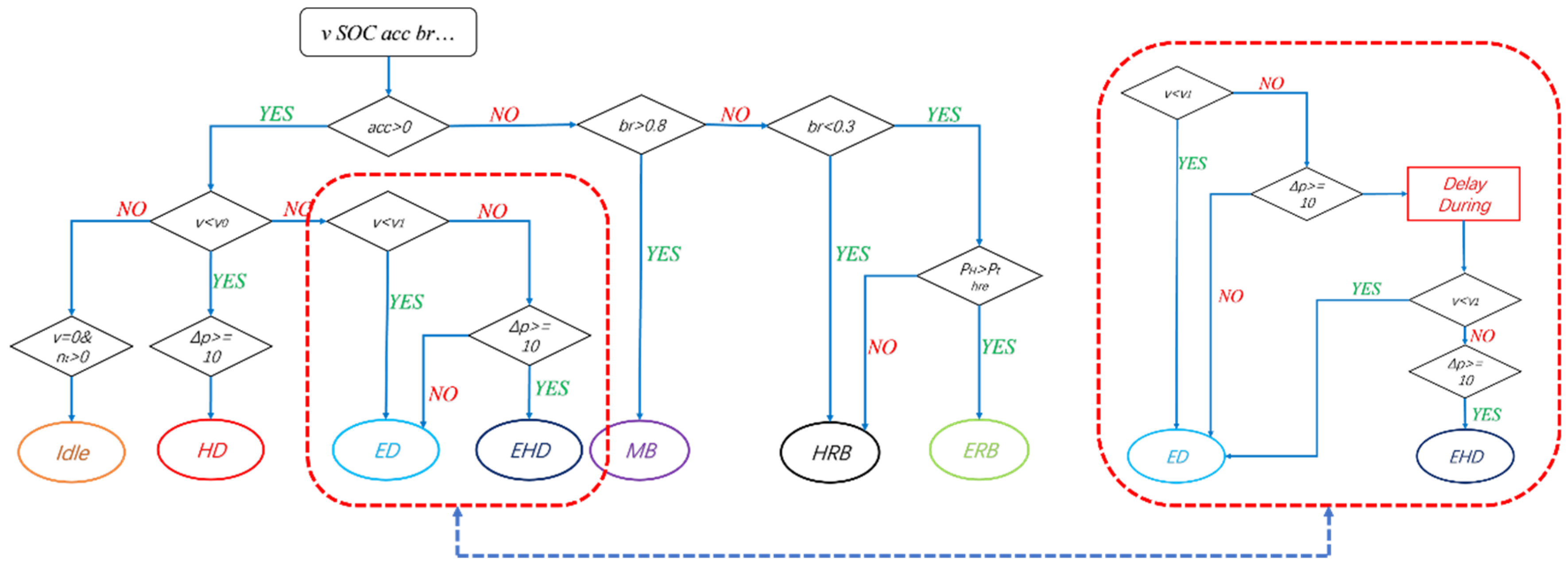
3.4. Simplified Diagram of Strategy Construction

The electromechanical–hydraulic-coupling electric vehicle is based on the desired vehicle speed as input signal and real-time monitoring of the battery SOC, pressure difference, and energy storage condition, thus, ensuring that the output torque can meet the torque required with the vehicle. Finally, these signals are used to regulate the swashplate opening of the hydraulic pump/motor and the output torque of the motor in real time to reasonably control the stability of the hydraulic power and the electric power when working together, thus, reducing the peak torque and achieving a smooth switch between its different working modes.

When the accelerator pedal signal acc is greater than 0, the vehicle is in drive mode. If the vehicle speed, v, is less than or equal to the low-speed threshold, v₀, and the pressure difference, Δp, is greater than or equal to 10 MPa, the vehicle enters the hydraulic power drive mode. At this point, the vehicle speed is low, and the hydraulic energy is sufficient, the electromechanical–hydraulic-power-coupled electric vehicle can be started using hydraulic power.

When the vehicle speed, v, is greater than the low-speed threshold value, v₀, but less than the high-speed threshold value, v₁, the vehicle enters the electric power drive mode, and only electric power is output.

When the vehicle speed, v, is greater than the high-speed threshold, v₁, the vehicle enters the electrohydraulic hybrid drive mode. At this point, the energy available from the hydraulics is not sufficient to meet the vehicle’s needs. Therefore, the electric power also starts to work, coupling with the hydraulic power for torque and outputting torque externally.

When v = 0 and the motor is not switched off, the vehicle enters the idle mode. At this point, the electromechanical–hydraulic power coupling does not output power externally; the electric power drives the hydraulic pump to work, internally converting electrical energy into hydraulic energy stored in the high-pressure accumulator for energy replenishment.

When the vehicle is braking, it is controlled according to the intensity signal, br, of the brake pedal and the high-pressure accumulator pressure, P_H. When the braking signal, br, is greater than 0.8, the vehicle enters mechanical braking mode, at which point no braking energy is recovered. When the brake signal, br, is less than 0.3 and the high-pressure accumulator pressure P_H is not sufficient, it enters the hydraulic-regenerative-braking mode; if the high-pressure accumulator pressure value, P_H, is greater than the pressure threshold, it means that the hydraulic energy is no longer recovered at which time it enters the motor regenerative braking mode. When the braking signal, br, is greater than 0.3 and less than 0.8, at this time, the pressure value of the high-pressure accumulator is judged first, and under the premise of meeting the requirements, hydraulic regenerative braking is carried out first; if there is surplus energy after the hydraulic energy is stored, then electric regenerative braking is carried out. The mode-switching process of the whole vehicle is shown in Figure 3.

The delay link is added when the vehicle speed reaches v₁. That is, when the vehicle wants to switch from ED mode to EHD mode, a duration decision is made first, and when the time is over, the speed value at the end is judged in relation to v₁. If the speed is still greater than v₁, the vehicle enters EHD mode. The battery and hydraulic motor drive the car forward together. If the speed is less than v₁, the vehicle should maintain the ED mode without moving, thus avoiding the frequent use of hydraulic components.

Shown in Figure 4 above are the vehicle controls, battery, motor, and hydraulic component parts (high- and low-pressure accumulators) via the control unit. In the original control strategy, the change in swashplate tilt angle through the road condition input and the electromechanical–hydraulic-coupling output varies dramatically at the places marked in the diagram and can be reduced more significantly by the inclusion of a time delay link.

In general, to avoid the impact of high current and high power on the battery, the vehicle enters HD mode when starting, receives an electromagnetic signal to open the swashplate, and the high-pressure oil flows into the low-pressure accumulator (LPA) through the hydraulic motor. The motor converts hydraulic energy into mechanical energy via the reciprocating movement of the plunger [32]. When the low-speed threshold is reached while driving, the vehicle switches from HD to ED mode, the swashplate begins to close, and the motor begins to output power to ensure normal vehicle operation. When the vehicle speed reaches the high-speed threshold, the vehicle automatically switches from ED mode to EHD mode. When accelerating, the required power of the vehicle is high. At this time, the hydraulic and electric torques are coupled in an appropriate ratio inside the electrohydraulic coupler, and then, the power is output through the rotating shaft. Thus, the electrical and hydraulic energies are converted into mechanical energy.

As shown in the figure above, the mode-switching strategy of electromechanical–hydraulic-power-coupled electric vehicles primarily relies on the vehicle speed threshold and the accumulator pressure value. When the road conditions appear around the speed threshold, and there are frequent fluctuations, it is bound to represent the inside of the electrohydraulic coupler. Frequent mode changes will also occur with frequent fluctuations in speed. To improve system reliability, a delay control module is added to the energy management strategy of the proposed basic rules. Considering ED and EHD modes as examples, when the high-speed threshold is reached, the system begins to switch from ED mode to EHD mode. During this period, a time delay determination (Γ) is set, and the power-switching sensitivity is reduced through the delay determination link.

4. Analysis of Basic Typical Road Conditions

The time delay between the ED and EHD modes is investigated as the research object. By entering classic road conditions (UDDS, NEDC, and WLTC) [33,34] using the AMEsim and Simulink cosimulation platform [35,36], the speed-following conditions and SOC changes can be described.

Figure 5 refers to the speed-following values at different delay times, in which six segments (A–F) are intercepted respectively to observe the speed-following condition [37] in which it can be seen that the speed-following condition basically does not change as the delay time increases or decreases, although there are very short localized periods of slow speed following, but in the vast majority of the time it is in full following condition, indicating that in the classical road conditions, the addition of delay links and the change of delay time did not have a significant impact on the speed-following situation.

Figure 6 refers to the final battery SOC values at different delay times, and time delays of 0.2 s were taken to observe the effect of delay time on the final battery SOC values [38] based on the histogram performance; the amount of change in the final battery SOC values was minimal with the highest final battery SOC value being 94.758% and the lowest being 94.751% under NEDC conditions with a very small difference of 0.007%. The highest final battery SOC value was 95.212% and the lowest was 95.202% under UDDS conditions with a great magnitude of 0.010%, and the highest final battery SOC value was 85.718% and the lowest was 85.703% under WLTC conditions with a great magnitude of 0.015%. The addition of the delay link and the change in delay time did not have a significant effect on the final battery SOC value under classical road conditions.

Figure 7 shows the sensitivity of the battery SOC to the delay time. The following figure shows the sensitivity of the battery SOC to the delay time, using the delay time of 0.5 s as the middle value of the delay time and the change in the delay time variable (±20%–±100%) based on the results obtained; the amount of change in the final battery SOC value remains largely between ±0.025%, indicating that the sensitivity of the final battery SOC value to the delay time variable is low.

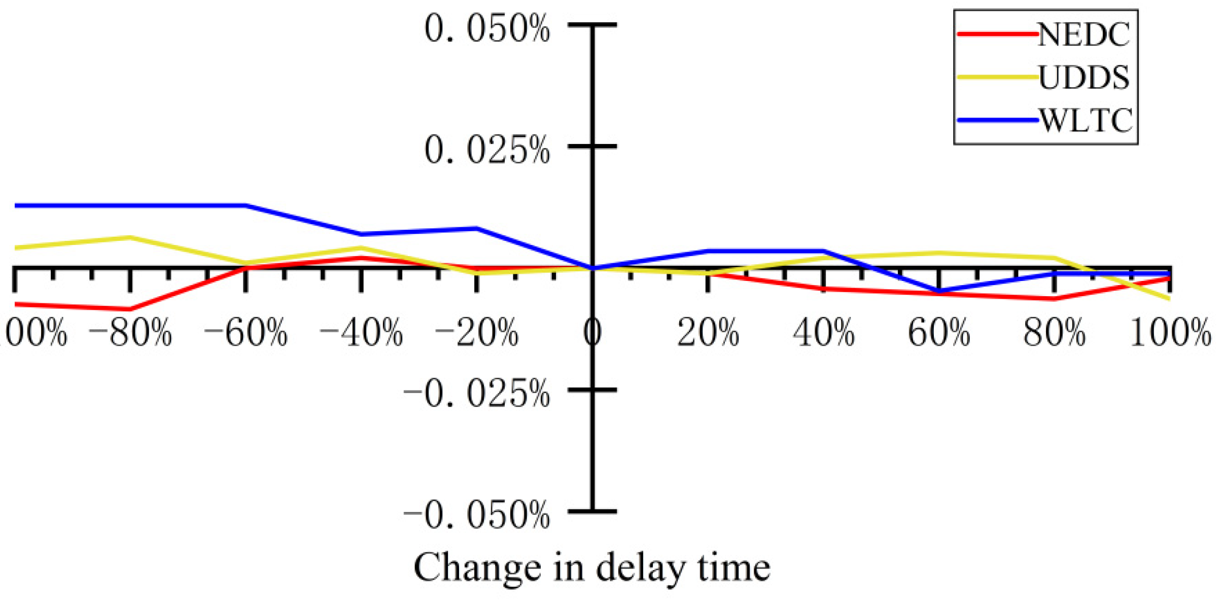
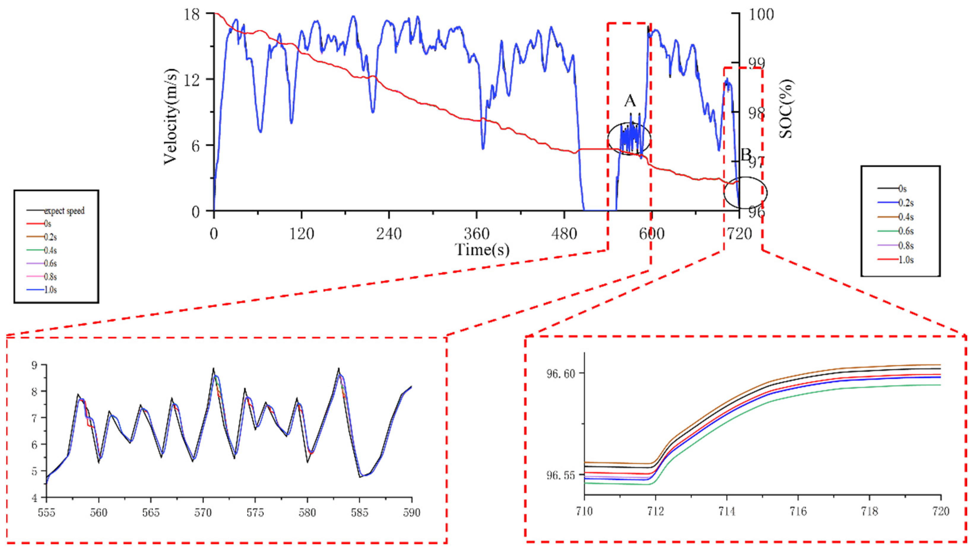
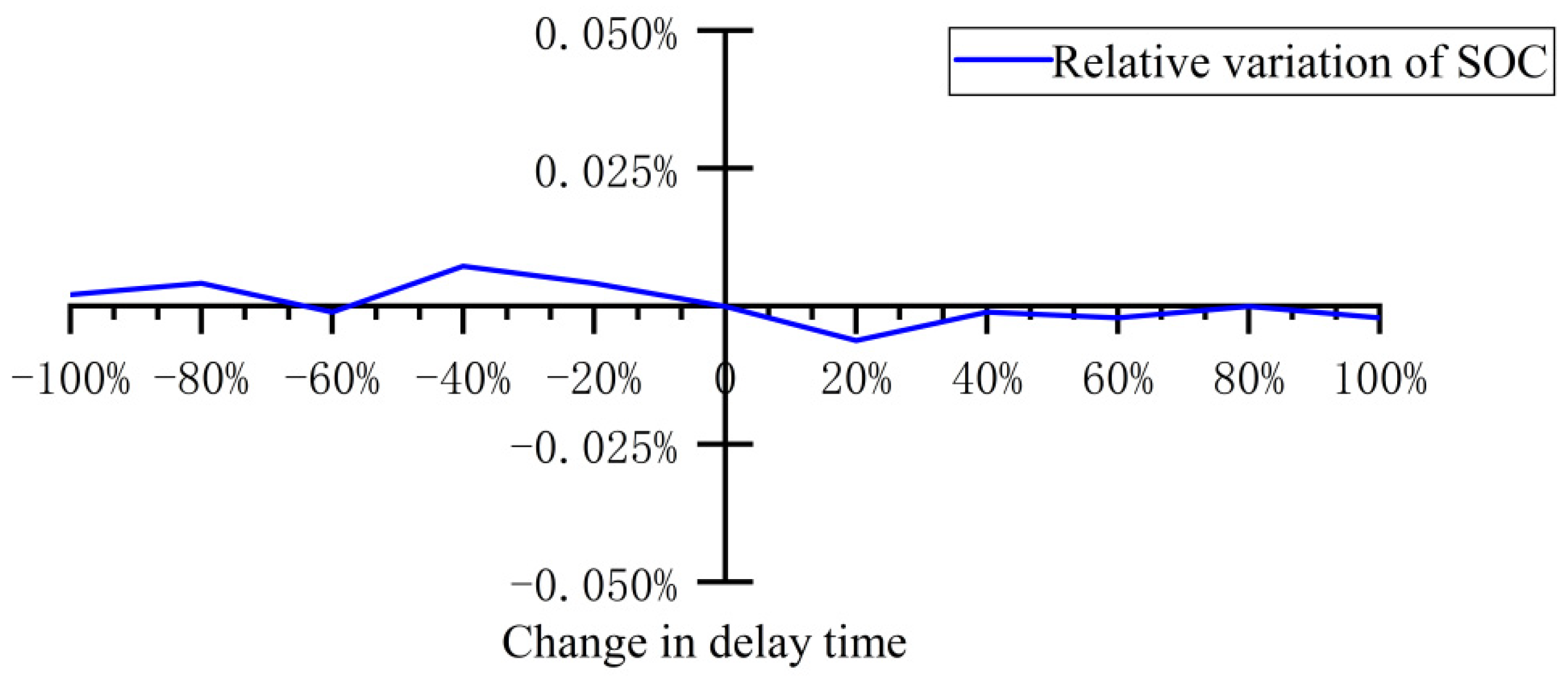
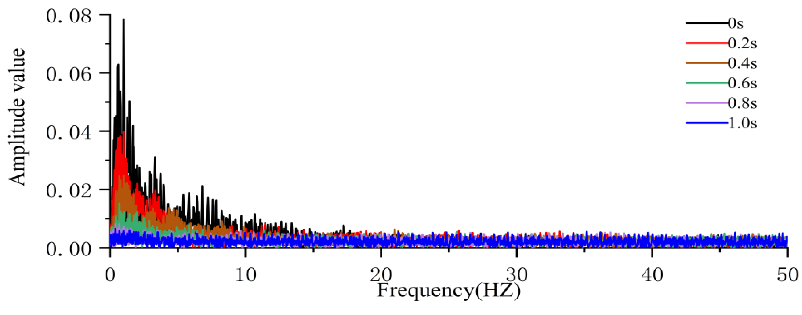
5. Verify the Feasibility of a Delay Control Strategy

To verify the feasibility of the delay control strategy, the delay control strategy was found to have almost no effect on the following conditions: the vehicle speed and the SOC value under typical operating conditions. In the real situation, vehicle speed frequently switches around the speed-switching threshold state, which allows us to verify the correctness and feasibility of the delay control strategy.

Figure 8 shows whether the different delay times have a significant effect on the vehicle speed following, and the final battery SOC value under frequent speed-switching road conditions is amount of change in the final value of SOC. From the enlarged graph of Circle A, it can be seen that the speed-following situation is relatively good. There is no delayed link or delay time change that causes the speed not to follow. There is no long-time ideal speed, and the actual speed difference is too large. It can be said that the overall speed-following situation is good. The graph in Box B shows that the change in delay time does have an effect on the final battery SOC value, as can be seen on the graph. The maximum final battery SOC value occurs at a delay time of 0.4 s, and the battery SOC value is 96.604%, while the minimum final battery SOC value occurs at a delay time of 0.6 s, and the battery SOC value is 96.594%, with a difference between the two of 0.010%. Although there is an effect, it can be seen that the change in the delay time value has a small effect on the final battery SOC value.

Figure 9 shows the sensitivity of the battery SOC to the delay time under this road condition, similar to the sensitivity to the classical road condition, using a delay time of 0.5 s as the middle value of the delay time, and using ±20%–±100% for the delay time variables, respectively, to observe the amount of change in the battery SOC. 0.025%, indicating that the sensitivity of the final battery SOC value to the delay time variable is indeed low.

Figure 10 shows the change in swashplate tilt angle for a given frequent speed condition by comparing the change in swashplate tilt angle for different delayed control times. When the value of the swashplate tilt angle is positive, it means that the hydraulic element is involved in the power output process, and the number of times the vehicle is in that drive mode can be judged by comparing the motor output curve when the value of the swashplate tilt angle is negative, it means that the hydraulic element is involved in the energy recovery process. From Figure 10 it can be seen with the change of vehicle speed that the swashplate inclination angle curve has a number of peaks up and down. From Figure 8, it can be derived that 555 s–590 s is the speed of the frequent stage change. The round box A represents the change of the swashplate inclination angle within this event. From the graph of the round box A, it can be found that there is no delay phase. The swashplate inclination angle of the positive direction of the change is more, it shows that the change in speed keeps adding more and more. The hydraulic power also enters the power output process briefly with the speed change when the valve value frequently switches, the delay module is added to the control strategy, and the delay time appears to change. The change of the positive direction of the swashplate tilt angle gradually decreases. From Figure 8, it is seen that the addition of the delay link and the change of the delay time have no greater influence on the vehicle speed-following situation and the battery SOC, thus, the delay in the link. The inclusion of the delay link can effectively reduce the number of hydraulic module engagements without affecting vehicle operation.

To describe more vividly the change in inclination of the swashplate from 555 s to 590 s, the plot of the change in inclination of the swashplate at times of 555 s–590 s shown in Figure 8 was processed with fast Fourier variation to obtain a plot that is easier to understand in the frequency domain [39,40,41].

A Fourier transform can transform any function into the sum of a series of sine/cosine functions. Any function refers to the vibration signal collected in this article, and the sine/cosine functions contain the frequency and corresponding amplitude information of the vibration signal. We assumed that the input vibration signal x(t)’s Fourier transform can be expressed as:

$$X\left(f\right)={\displaystyle {\int }_{-\infty }^{\infty }x\left(t\right)}{e}^{-j2\pi ft}dt$$

(15)

where t is time and f is frequency.

The fast Fourier transform (FFT) algorithm is orders of magnitude more efficient than the discrete Fourier transform (DFT). FFT can extract the frequency from the collected vibration signal, which is expressed as a time domain signal, the horizontal axis is the time or sampling point, and the vertical axis is the amplitude, forming a frequency domain map where the horizontal axis is the frequency and the vertical axis is the amplitude. The FFT algorithm expression is as follows:

$$\{\begin{array}{l}X\left(k\right)=X_1\left(k\right)+w_N^k{X}_2\left(k\right)\\ X\left(k+N/2\right)=X_1\left(k\right)-w_N^k{X}_2\left(k\right)\end{array},k=0,1\dots ,N/2-1,N=2^M$$

(16)

Figure 11 shows the frequency domain distribution obtained from Figure 10 by FFT. It can be seen that with the addition of the delay link, the amplitude of the swashplate tilt angle in the low frequency band has a significant reduction and improvement effect, and also reflects the gradual reduction of the change in the positive direction in the time domain distribution, which can also be concluded without affecting the vehicle specific It also reflects the gradual reduction of the positive directional variation in the time domain distribution, which can be concluded that the mode-switching frequency is suppressed without affecting the specific driving conditions of the vehicle.

Figure 12 shows the sensitivity of the average amplitude value to the delay time under this road condition, similar to the sensitivity to the battery SOC analysis, using the delay time of 0.5 s as the middle value of the delay time, and using ±20%–±100%, respectively, to observe the change of the average amplitude value. When the delay time variable was changed negatively, the change in the mean amplitude was always more obvious, but when it was changed in the positive direction, the change was obvious when the increase was 0%–60%, and the change was smaller when the increase was 60%–100%, which means that after the amplitude exceeded 60%, the increase in the amplitude was difficult to cause the fluctuation of the mean amplitude of large values, and the sensitivity of the battery SOC to the delay time differed greatly from the above analysis, which means that the mean amplitude mean is indeed more sensitive to the delay time variable, and is also a side reflection of the fact that the addition of the delay link and the increase in delay time has a significant inhibiting effect on the switching of vehicle operating modes.

6. Conclusions

To improve the reliability of the system and reduce the sensitivity of power switching, this study reduces the mode-switching frequency by adding a delay control module to the control strategy link, taking into account the established electrohydraulic-power-coupled electric vehicle model.

Simulation results show that within a certain delay control time, adding a delay control link has little effect on the driving of electrohydraulic-power-coupled electric vehicles under classical road conditions. Through a sensitive analysis, it can also be found that the change in delay time has a small effect on the speed-following situation and battery SOC; for road conditions with frequent changes near the speed threshold, through sensitive analysis, it can be found that different delay control times will have different effects on the road conditions with frequent changes around the speed threshold. A sensitive analysis reveals that different delay control times have different effects on the switching frequency of the modes, but compared to the effects of speed following and battery SOC, adding delay control links can effectively reduce the switching frequency between different modes.

The disadvantage is that due to the uncertainty of the vehicle road conditions, the effect of different delay times on the switching frequency of the vehicle can only be analysed, and it can be determined that the addition of the delay link has a significant effect on the switching frequency of the modes, but an optimal delay control time cannot be derived to minimise the mode control frequency.

The next step should be to try to introduce some optimisation algorithms to optimise the time value of the delay link to expect better results.

References

1. Zhou, Y.; Ravey, A.; Péra, M.-C. Multi-objective energy management for fuel cell electric vehicles using online-learning enhanced Markov speed predictor. Energy Convers. Manag. 2020, 213, 112821. [Google Scholar]
2. Hong, J.; Wang, Z.; Chen, W.; Wang, L.; Lin, P.; Qu, C. Online accurate state of health estimation for battery systems on real-world electric vehicles with variable driving conditions considered. J. Clean. Prod. 2021, 294, 125814. [Google Scholar] [CrossRef]
3. Wu, W.; Hu, J.; Yuan, S.; Di, C. A hydraulic hybrid propulsion method for automobiles with self-adaptive system. Energy 2016, 114, 683–692. [Google Scholar] [CrossRef]
4. Xia, L.; Quan, L.; Ge, L.; Hao, Y. Energy efficiency analysis of integrated drive and energy recuperation system for hydraulic excavator boom. Energy Convers. Manag. 2018, 156, 680–687. [Google Scholar] [CrossRef]
5. He, X.; Xiao, G.; Hu, B.; Tan, L.; Tang, H.; He, S.; He, Z. The applications of energy regeneration and conversion technologies based on hydraulic transmission systems: A review. Energy Convers. Manag. 2019, 205, 112413. [Google Scholar]
6. Hong, J.; Wang, Z.; Yao, Y. Fault prognosis of battery system based on accurate voltage abnormity prognosis using long short-term memory neural networks. Appl. Energy 2019, 251, 113381. [Google Scholar] [CrossRef]
7. Lu, X.; Chen, Y.; Wang, H. Multi-Objective Optimization Based Real-Time Control for PEV Hybrid Energy Management Systems. In Proceedings of the IEEE Applied Power Electronics Conference and Exposition (APEC), San Antonio, TX, USA, 4–8 March 2018. [Google Scholar]
8. Hong, J.; Wang, Z.; Chen, W.; Yao, Y. Synchronous multi-parameter prediction of battery systems on electric vehicles using long short-term memory networks. Appl. Energy 2019, 254, 113648. [Google Scholar] [CrossRef]
9. Liu, H.; Chen, G.; Xie, C.; Li, D.; Wang, J.; Li, S. Research on energy-saving characteristics of battery-powered electric-hydrostatic hydraulic hybrid rail vehicles. Energy 2020, 205, 118079. [Google Scholar] [CrossRef]
10. Liu, H.; Jiang, Y.; Li, S. Design and downhill speed control of an electric-hydrostatic hydraulic hybrid powertrain in battery-powered rail vehicles. Energy 2019, 187, 115957. [Google Scholar] [CrossRef]
11. Hu, J.; Mei, B.; Peng, H.; Guo, Z. Discretely variable speed ratio control strategy for continuously variable transmission system considering hydraulic energy loss. Energy 2019, 180, 714–727. [Google Scholar] [CrossRef]
12. Gong, J.; Zhang, D.; Guo, Y.; Liu, C.; Zhao, Y.; Hu, P.; Quan, W. Power control strategy and performance evaluation of a novel electro-hydraulic energy-saving system. Appl. Energy 2018, 233–234, 724–734. [Google Scholar] [CrossRef]
13. Yang, J.; Zhang, T.; Hong, J.; Zhang, H.; Zhao, Q.; Meng, Z. Research on Driving Control Strategy and Fuzzy Logic Optimization of a Novel Mechatronics-Electro-Hydraulic Power Coupling Electric Vehicle. Energy 2021, 233, 121221. [Google Scholar] [CrossRef]
14. Hong, J.; Ma, F.; Xu, X.; Yang, J.; Zhang, H. A novel mechanical-electric-hydraulic power coupling electric vehicle considering different electrohydraulic distribution ratios. Energy Convers. Manag. 2021, 249, 114870. [Google Scholar] [CrossRef]
15. Yang, J.; Zhang, T.; Zhang, H.; Hong, J.; Meng, Z. Research on the Starting Acceleration Characteristics of a New Mechanical–Electric–Hydraulic Power Coupling Electric Vehicle. Energies 2020, 13, 6279. [Google Scholar] [CrossRef]
16. Brol, S.; Czok, R.; Mróz, P. Control of energy conversion and flow in hydraulic-pneumatic system. Energy 2019, 194, 116849. [Google Scholar] [CrossRef]
17. Zhao, Q.; Zhang, H.; Xin, Y. Research on Control Strategy of Hydraulic Regenerative Braking of Electrohydraulic Hybrid Electric Vehicles. Math. Probl. Eng. 2021, 2021, 5391351. [Google Scholar] [CrossRef]
18. Xiong, W.; Zhang, Y.; Yin, C. Optimal energy management for a series–parallel hybrid electric bus. Energy Convers. Manag. 2009, 50, 1730–1738. [Google Scholar] [CrossRef]
19. He, H.; Wang, C.; Jia, H.; Cui, X. An intelligent braking system composed single-pedal and multi-objective optimization neural network braking control strategies for electric vehicle. Appl. Energy 2019, 259, 114172. [Google Scholar] [CrossRef]
20. Hong, J.; Wang, Z.; Ma, F.; Yang, J.; Xu, X.; Qu, C.; Zhang, J.; Shan, T.; Hou, Y.; Zhou, Y. Thermal Runaway Prognosis of Battery Systems Using the Modified Multiscale Entropy in Real-World Electric Vehicles. IEEE Trans. Transp. Electrif. 2021, 7, 2269–2278. [Google Scholar] [CrossRef]
21. Zeng, X.; Wu, Z.; Wang, Y.; Song, D.; Li, G. Multi-mode energy management strategy for hydraulic hub-motor auxiliary system based on improved global optimization algorithm. Sci. China Technol. Sci. 2020, 63, 2082–2097. [Google Scholar] [CrossRef]
22. Hong, J.; Wang, Z.; Zhang, T.; Yin, H.; Zhang, H.; Huo, W.; Zhang, Y.; Li, Y. Research on integration simulation and balance control of a novel load isolated pure electric driving system. Energy 2019, 189, 116220. [Google Scholar] [CrossRef]
23. Li, B.; Bei, S. Estimation algorithm research for lithium battery SOC in electric vehicles based on adaptive unscented Kalman filter. Neural Comput. Appl. 2018, 31, 8171–8183. [Google Scholar] [CrossRef]
24. Wu, W.; Hu, J.; Jing, C.; Jiang, Z.; Yuan, S. Investigation of energy efficient hydraulic hybrid propulsion system for automobiles. Energy 2014, 73, 497–505. [Google Scholar] [CrossRef]
25. Aymen, F.; Novak, M.; Lassaad, S. An improved reactive power MRAS speed estimator with optimization for a hybrid electric vehicles application. J. Dyn. Syst. Meas. Control. 2018, 140, 061016. [Google Scholar] [CrossRef]
26. Aymen, F.; Berkati, O.; Lassaad, S.; Srifi, M.N. BLDC control method optimized by PSO algorithm. In Proceedings of the 2019 International Symposium on Advanced Electrical and Communication Technologies (ISAECT), Rome, Italy, 27–29 November 2019; pp. 1–5. [Google Scholar]
27. Naoui, M.; Aymen, F.; Mouna, B.H.; Sbita, L. Brushless Motor and Wireless Recharge System for Electric Vehicle Design Modeling and Control. In Handbook of Research on Modeling, Analysis, and Control of Complex Systems; IGI Global: Hershey, PA, USA, 2020. [Google Scholar]
28. Gao, J.P.; Wei, Y.H.; Liu, Z.N.; Qiao, H.B. Matching and optimization for powertrain system of parallel hybrid electric vehicle. Appl. Mech. Mater. 2013, 341–342, 423–431. [Google Scholar]
29. Mu, Y.; Zhou, G.; Hou, D.; Zhu, M.; Xu, Y.; Song, N.; Gao, J. Parameter Matching and Simulation of Plug-in Hybrid Electric Bus. In Proceedings of the 2019 2nd International Conference on Information Systems and Computer Aided Education (ICISCAE), Dearborn, MI, USA, 7–10 September 2009; pp. 446–451. [Google Scholar]
30. Khare, N.; Chandra, S.; Govil, R. Statistical modeling of SoH of an automotive battery for online indication. In Proceedings of the INTELEC 2008–2008 IEEE 30th International Telecommunications Energy Conference, San Diego, CA, USA, 14–18 September 2008. [Google Scholar]
31. Miroslaw, T.; Szlagowski, J.; Zawadzki, A.; Zebrowski, Z. Simulation model of an off-road four-wheel-driven electric vehicle. Proc. Inst. Mech. Eng. Part I J. Syst. Control. Eng. 2018, 233, 1248–1262. [Google Scholar] [CrossRef]
32. Kamal, E.; Adouane, L. Hierarchical Energy Optimization Strategy and Its Integrated Reliable Battery Fault Management for Hybrid Hydraulic-Electric Vehicle. IEEE Trans. Veh. Technol. 2018, 67, 3740–3754. [Google Scholar] [CrossRef]
33. Işıklı, F.; Sürmen, A.; Gelen, A. Modelling and Performance Analysis of an Electric Vehicle Powered by a PEM Fuel Cell on New European Driving Cycle (NEDC). Arab. J. Sci. Eng. 2021, 46, 7597–7609. [Google Scholar] [CrossRef]
34. Kuittinen, N.; McCaffery, C.; Peng, W.; Zimmerman, S.; Roth, P.; Simonen, P.; Karjalainen, P.; Keskinen, J.; Cocker, D.R.; Durbin, T.D.; et al. Effects of driving conditions on secondary aerosol formation from a GDI vehicle using an oxidation flow reactor. Environ. Pollut. 2021, 282, 117069. [Google Scholar] [CrossRef]
35. Li, H.; Li, S.; Sun, W.; Wang, L.; Lv, D. The optimum matching control and dynamic analysis for air suspension of multi-axle vehicles with anti-roll hydraulically interconnected system. Mech. Syst. Signal Process. 2020, 139, 106605. [Google Scholar] [CrossRef]
36. Chen, Y.; Li, C.; Chen, S.; Ren, H.; Gao, Z. A combined robust approach based onauto-regressive longshort-term memory network and moving horizon estimation for state-of-charge estimation of lithium-ion batteries. Int. J. Energy Res. 2021, 45, 12838–12853. [Google Scholar] [CrossRef]
37. Xie, J.; Xu, X.; Wang, F.; Tang, Z.; Chen, L. Coordinated control based path following of distributed drive autonomous electric vehicles with yaw-moment control. Control Eng. Pract. 2020, 106, 104659. [Google Scholar] [CrossRef]
38. Ouyang, Q.; Han, W.; Zou, C.; Xu, G.; Wang, Z. Cell Balancing Control For Lithium-Ion Battery Packs: A Hierarchical Optimal Approach. IEEE Trans. Ind. Inform. 2019, 16, 5065–5075. [Google Scholar] [CrossRef]
39. Liu, S.; Shan, T.; Tao, R.; Zhang, Y.D.; Zhang, G.; Zhang, F.; Wang, Y. Sparse Discrete Fractional Fourier Transform and Its Applications. IEEE Trans. Signal Process. 2014, 62, 6582–6595. [Google Scholar] [CrossRef] [Green Version]
40. Schlegel, M.; Škarda, R.; Čech, M. Running discrete Fourier transform and its applications in control loop performance assessment. In Proceedings of the 2013 International Conference on Process Control (PC), Strbske Pleso, Slovakia, 18–21 June 2013. [Google Scholar]
41. Tao, R.; Li, Y.-L.; Wang, Y. Short-Time Fractional Fourier Transform and Its Applications. IEEE Trans. Signal Process. 2009, 58, 2568–2580. [Google Scholar] [CrossRef]
Figure 1. Schematic showing the structural principles of the electrohydraulic coupler. 1, front cover; 2, return disc; 3, plunger; 4, diaphragm spring; 5, stator core; 6, stator winding; 7, housing; 8, transmission shaft; 9, spherical spring seat; 10, swashplate; 11, slide shoe; 12, permanent magnet; 13, guide sleeve; 14, cylinder block; 15, distribution plate; U1, U2, U3, lead terminal.
Electronics 11 01299 g001
Figure 2. Structure of an electrohydraulic-power-coupled electric vehicle.
Electronics 11 01299 g002
Figure 3. Flow chart for mode switching.
Electronics 11 01299 g003
Figure 4. Initial control strategy diagram.
Electronics 11 01299 g004
Figure 5. Velocity values under different delay times.
Electronics 11 01299 g005
Figure 6. SOC values at different delay times.
Electronics 11 01299 g006
Figure 7. Sensitivity analysis of delay time values to SOC under different road conditions.
Electronics 11 01299 g007
Figure 8. Speed values and SOC with different delay times under real operating conditions.
Electronics 11 01299 g008
Figure 9. Sensitivity analysis of delay time values to SOC under road conditions.
Electronics 11 01299 g009
Figure 10. Variation in the tilt angle of the swashplate with different delay times under real working conditions.
Electronics 11 01299 g010
Figure 11. Swashplate inclination variation frequency domain curve for 555 s–590 s.
Electronics 11 01299 g011
Figure 12. Sensitivity analysis of delay time values to amplitude averages.
Electronics 11 01299 g012