1. Introduction
Wind energy is the fastest-growing renewable energy technology among other renewable energies. The global installed capacity of onshore wind power in 2018 was 542 GW, which will increase three-fold by 2030 (to 1787 GW) and ten-fold by 2050 (to 5044 GW) [
1]. The abundance of clean wind energy on the earth’s surface and the rapid developments in technology promises such high growth rate. Most wind energy conversion systems (WECS) integrated into the power grids are variable-speed wind turbine systems (VSWTS), due to their significant advantages over other wind turbine systems (WTS) [
2].
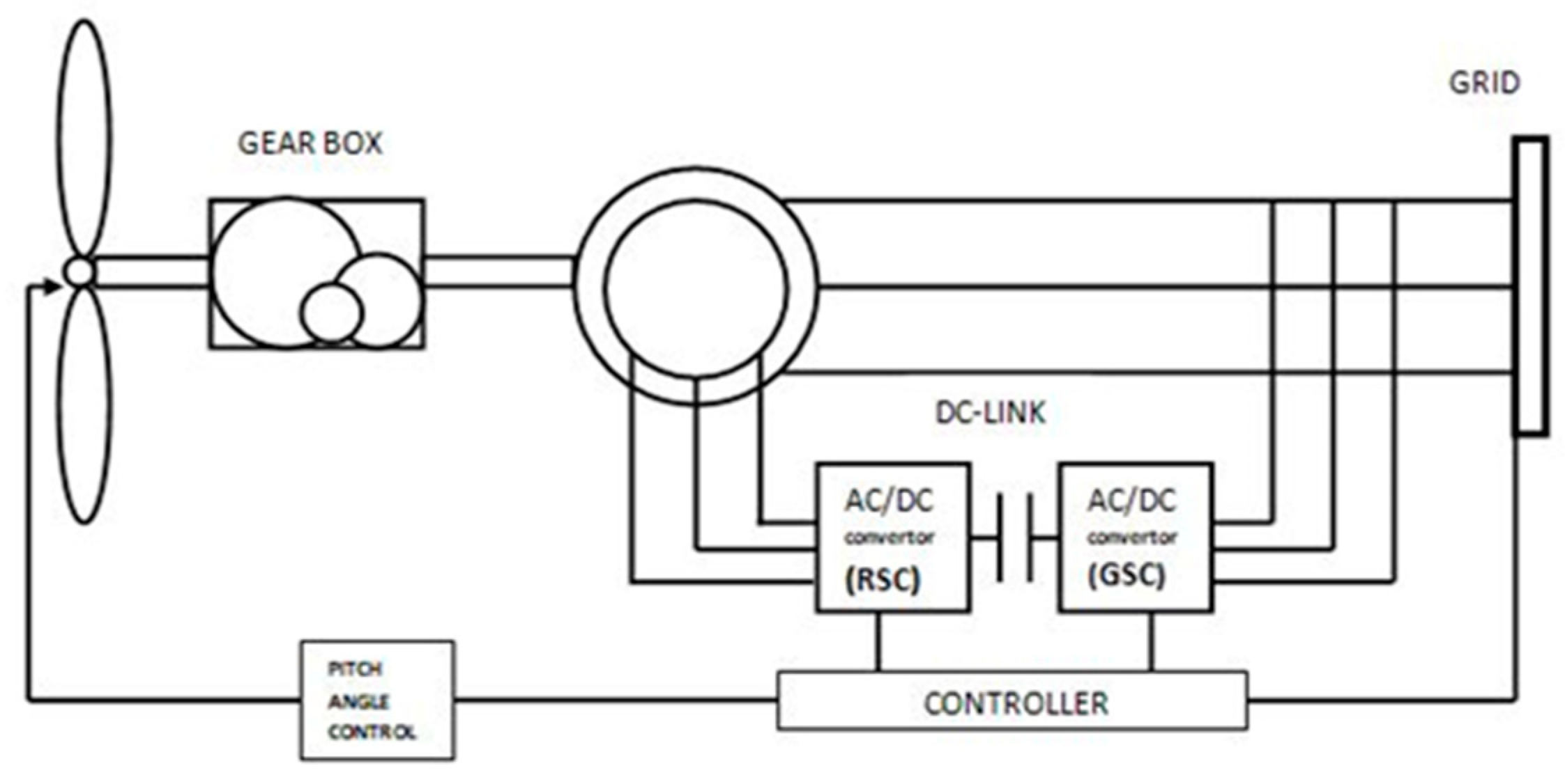
The doubly-fed induction generator (DFIG) is the most popular variable-speed generator used in WECS. The configuration of VSWTS with DFIG is shown in
Figure 1; in such a configuration, the stator windings of DFIG are directly connected to the grid, and the rotor windings are fed through a partially rated power electronic convertor system [
3]; usually, the convertor operates on less power—20–25% of the rated power [
4].
The control system of DFIG has significant importance in achieving good quality and maximum power from wind energy at different wind speeds. DFIG-based WTS has high nonlinearities and complexities due to unpredictable wind penetrations and a complex mechanical to electrical model. To overcome the problems in attaining good quality power in uncertain conditions, many nonlinear and adaptive approaches have been made to improve the control system. For convertor control, sliding mode control (SMC) is used in [
5]. The power control of DFIG via output feedback is discussed in [
6,
7]. A model reference adaptive system (MRAS) observer for sensorless control of DFIG is addressed in [
8]. The perturbation and observation (P&O) method is proposed in [
9] to improve power flow under fast variations of wind. For maximum power point tracking of DFIG, the grouped gray wolf optimizer (GWO) is used in [
10].
Pitch angle control is an essential part of the control system in VSWTS, where rated power is determined at rated wind speed. Different control schemes in [
11,
12,
13,
14] for VSWTS are suggested and applied to improve the response and control operations of the system.
This paper proposed computational optimization techniques to enhance the performance of the pitch angle controller by tuning the P and PI controllers used in pitch angle control operation. A multi-objective, multi-dimensional error function is minimized, not by the weighted sum method used in the previous articulating of preference methods in multi-objective optimization (MOO) [
15], but rather by selecting appropriate error criterion for each objective of the function that depicts the relative magnitude of each objective in the error function.
2. Wind Turbine Model
A simple model of a wind turbine will extract wind power and convert it into mechanical power. The wind power can be computed as [
16]:
where
is air density (1.225 kg/m
3 at 15 °C and normal pressure),
A is the swept area, or area of blades, and
v is the wind velocity.
The mechanical power
is obtained from the wind power
and depends upon the power coefficient
and is defined as [
16]
where
is a function of tip speed ratio
λ and pitch angle
β and is defined as [
17]
where
β is the pitch angle, and tip speed ratio
λ is defined as
where
is the rotational speed of the wind turbine rotor in p.u.
R is the radius of the swept area in
m and
is the speed of the wind and
is expressed as
The determines, how much wind power can be extracted from an air stream and its maximum value is defined by the Betz limit, which states that only 59.3% of the power from an airstream can be extracted. Practically, wind turbines have up to 50%.
3. Pitch Angle Control
Pitch angle control is the easy way to regulate the aerodynamic pressures on the wind turbine rotor blades when wind speed is beyond the rated speed [
18]. It enables servo operations which adjust the pitch of the blade according to wind velocity to extract optimal wind power. For DFIG-based wind turbines, different pitch angle controller designs have been proposed in [
19,
20,
21,
22].
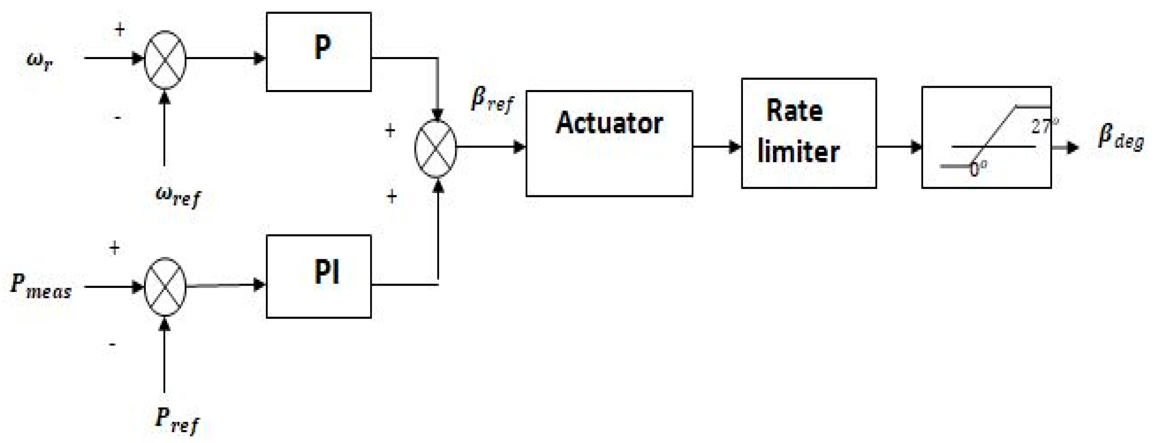
Pitch angle control is achieved using P and PI-controllers that feed the reference pitch signal to the actuator to enable the servo motor and change the pitch angle by the desire value [
23].
Figure 2 shows an open-loop pitch angle control model with a rate-limited actuator.
Two error signals, and , are connected to P and PI controllers, respectively. is the difference between the generator rotor speed () and its reference value () and is the difference between the measured turbine system power () and the reference power (). The controllers use proportional and integral gains to process the error signals. is the P-controller gain, referred to as pitch control gain. and are the PI-controller gains, referred to as pitch compensation gains. The controllers process the error signals to generate a reference pitch signal.
The system is limited as:
For a better dynamic response of the pitch angle controller, the parameters
,
, and
must be tuned properly; but due to the non-linearity and high complexity of the system, it is very difficult to find the optimal values of these parameters traditionally [
24]. Several computational optimization techniques can be used to find the optimal values of these parameters.
4. Computational Optimization Techniques
Modelling, simulation, and computational optimization are the three requirements in modern-design practices. Optimization techniques are used in all quantitative disciplines of the contemporary world [
25]. Computational optimization techniques are used for finding or selecting the best possible solution from a set of possible solutions. Different algorithms for optimization have been developed and applied since the inception of computational optimization.
The most popular algorithms for optimizing nonlinear and high complexity problems are particle swarm optimization (PSO) and genetic algorithm (GA). These algorithms are overviewed as:
4.1. Particle Swarm Optimization
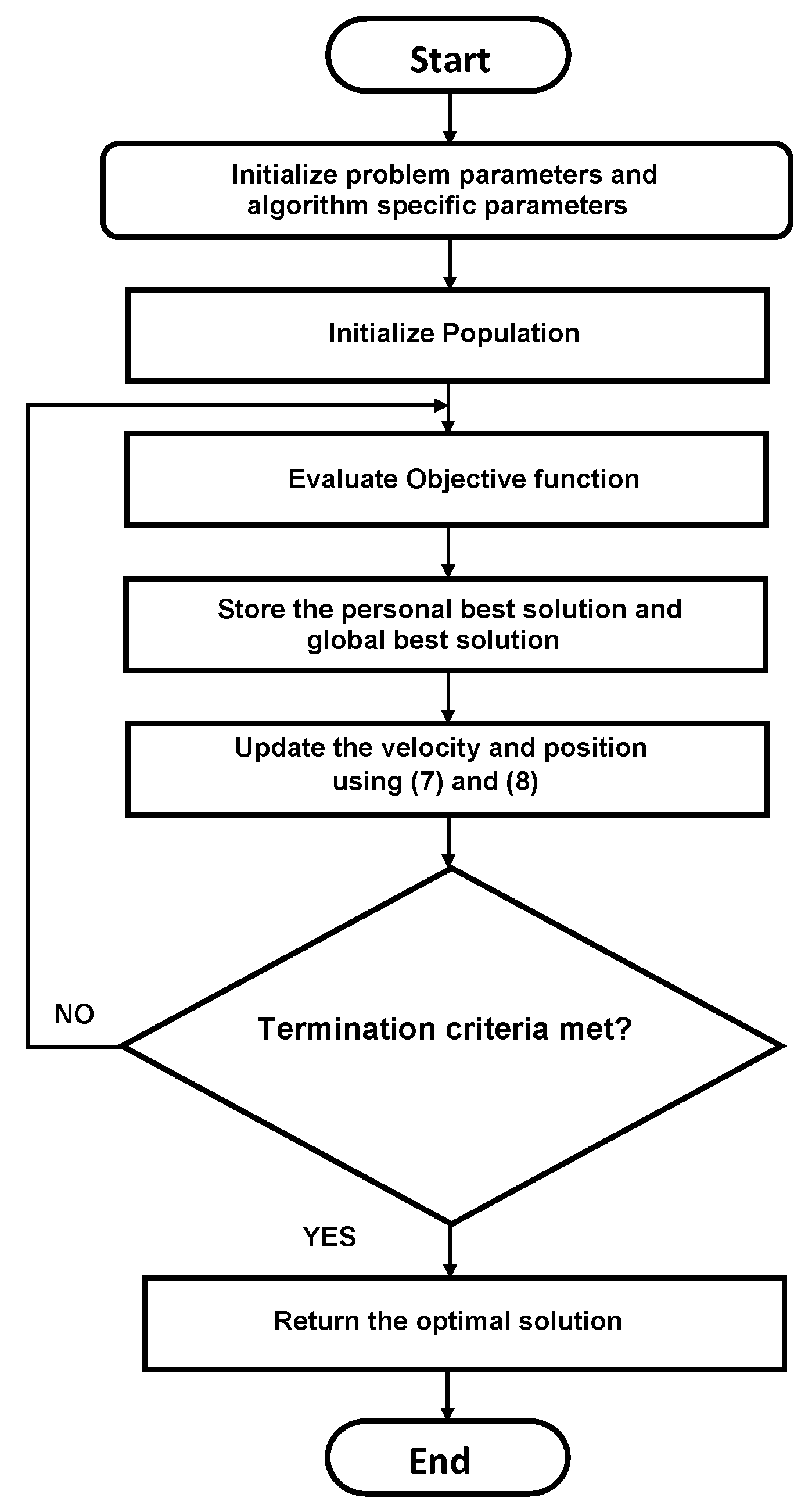
PSO was developed by Kennedy and Eberhart in 1995 [
26]. PSO is a stochastic optimization technique that is based on population and which virtually imitates bird flocking or fish schooling behaviours. PSO searches for the best possible solution from a number of moving particles. Each particle has a position in the problem space and represents a potential solution. The particles can be represented via a position vector
. The velocity of the moving swarm particles in the problem space can be represented via the velocity vector
. At each time,
is utilized to compute the fitness/objective function
. Every particle keeps track of its best position, which is represented via
(personal best). The best position among the entire swarm is also tracked and represented via
(global best). The positions of the particles in each iteration t are updated as follows:
The velocities of the particles in each iteration
t are updated as follows;
In the velocity update equation,
is the inertia, and
and
are random numbers which are uniformly distributed within the range of 0 and 1;
and
are acceleration coefficients. The velocity
is limited by
. PSO can be utilized for single, as well as for multi-objective nonlinear optimization problems [
27]. The algorithm is terminated once the optimal solution is found to the desired accuracy or a certain number of iterations are met. The flow diagram of the PSO algorithm is depicted in
Figure 3.
4.2. Genetic Algorithm
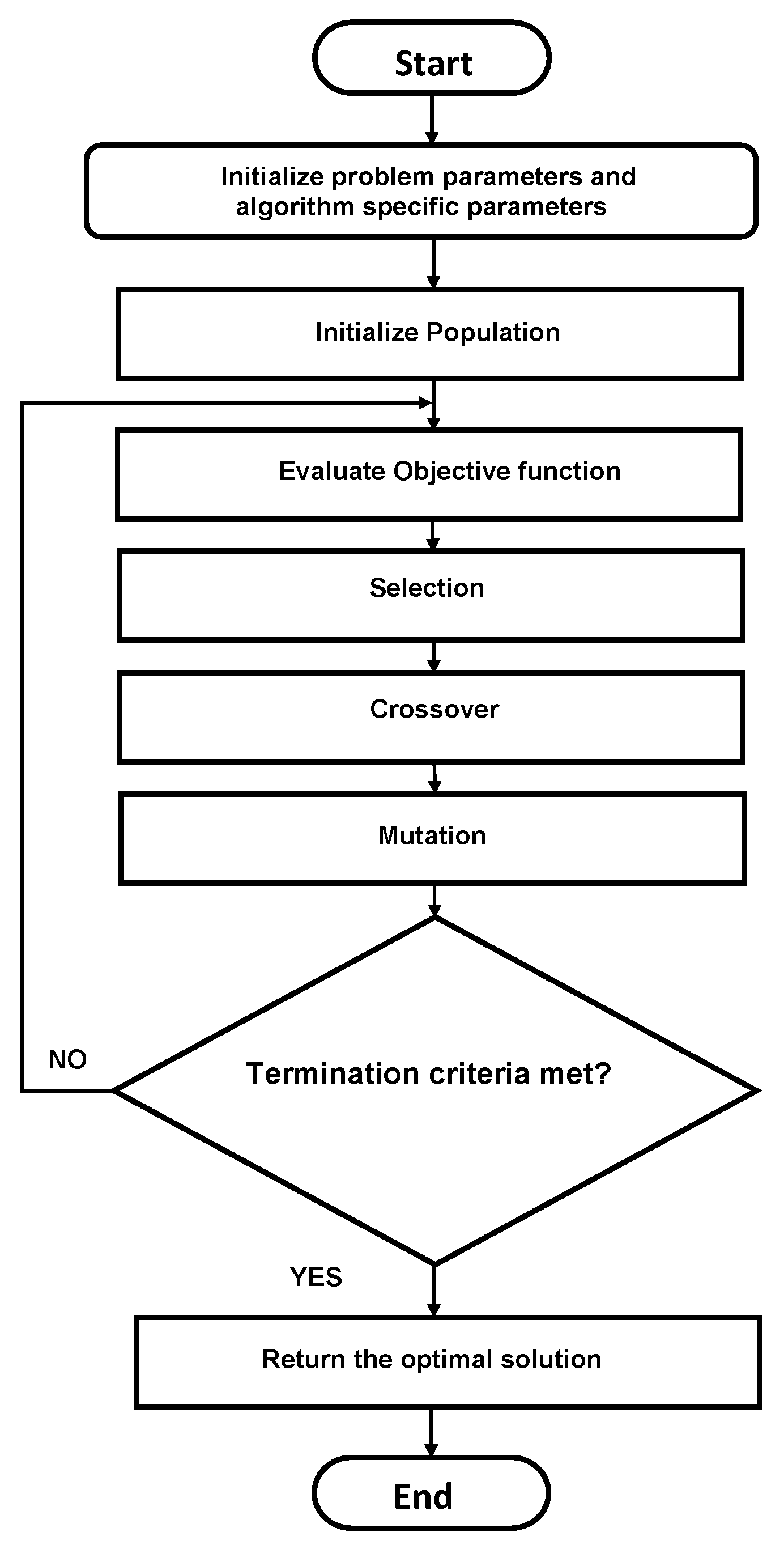
Genetic algorithms are inspired by the processes involved in natural evolution, which follows the Darwinian principle of the ‘survival of the fittest.’ The GA simulates the principle of survival of the fittest amongst individuals over a consecutive generation. Each generation has a population of individuals represented by character strings. Each individual represents a point in the problem space and a potential solution. The individuals in the population go through the process of evolution. The individuals compete for resources and mates. The individuals that perform well will stand out and reproduce more than others. From the individuals that perform well, genes will propagate so that higher-quality offspring are produced in the future. Thus, each successive generation’s quality is improved. The process of evolution is comprised of three stages, i.e., selection, crossover, and mutation, as depicted in the flow diagram of
Figure 4. The crossover and mutation process is scaled by defining the crossover and mutation probabilities.
Generally, binary string is used in GA to represent a problem solution, and for that purpose ‘encoding’ is very crucial. It has a major impact on the performance of GA. For binary representation, the determination of number of bits is very important.
The length of a binary string for an integer number
is given by:
The binary representation of any integer number
can be expressed as:
where
m is the given accuracy,
C is the coefficient and
L is the length of a binary string.
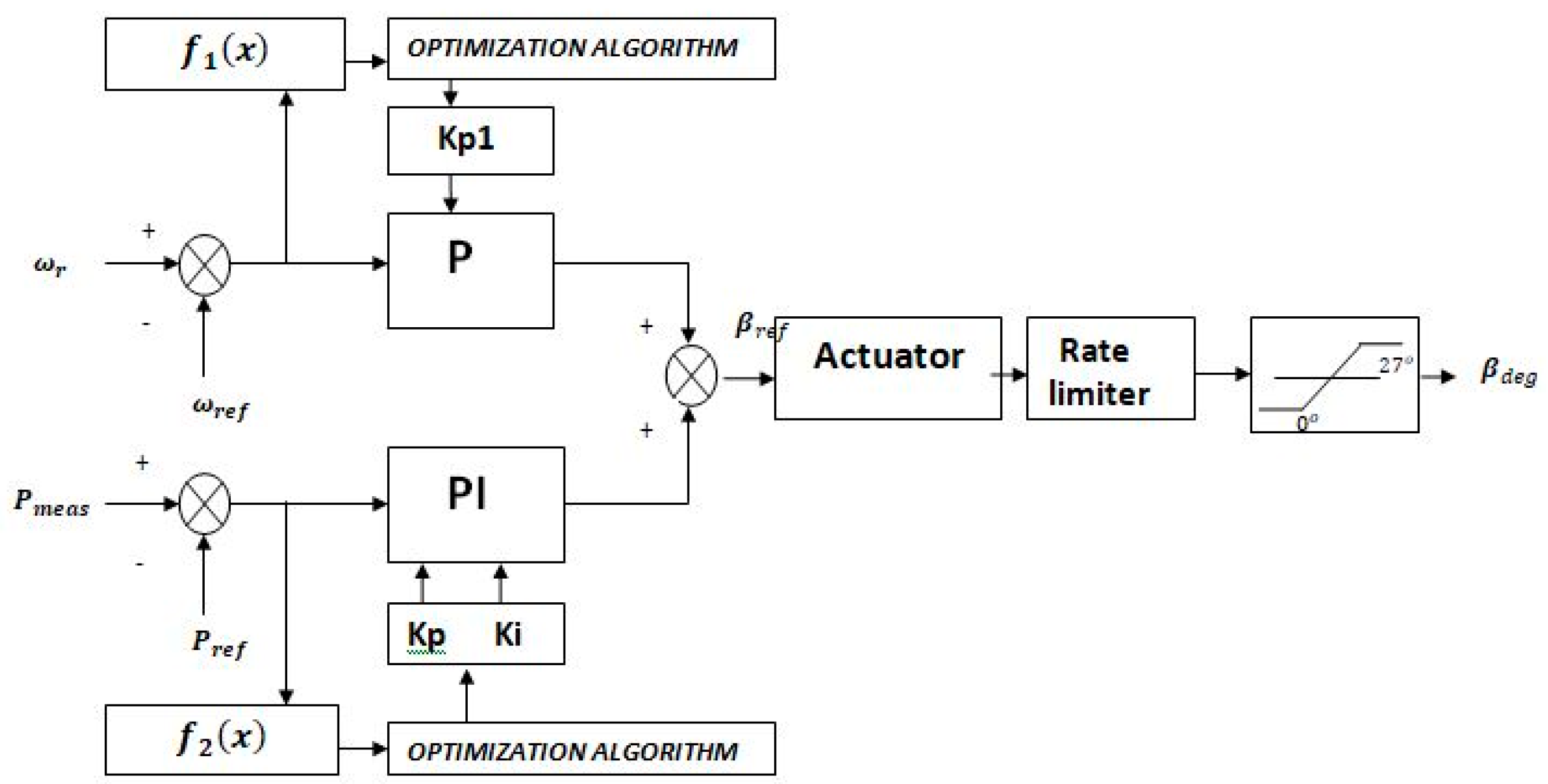
5. Optimal Pitch Angle Control
To find the optimal values of the control parameters, the pitch control gain (
) and pitch compensation gains (
and
) of the pitch angle control system model using optimization techniques, the objective or fitness function
f(
X) must be defined. A schematic diagram of the optimum pitch angle control is presented in
Figure 5. Generating a reference pitch signal is a multi-task operation in the control model, as it utilizes two error signals
e1 and
e2 which are processed by the P and PI controllers, respectively. A multi-objective, multi-dimensional function is designed to obtain a Pareto-optimal solution. The function is comprised of two objectives:
where
.
This multi-objective error function contours a multi-objective optimization (MOO) problem. In MOO problems, Pareto optimality is tricky to attain. The weighted sum method is extensively used for MOO to achieve a Pareto-optimal solution, which reflects decision-making preferences [
15]. However, to narrate the true presumptions, different weights for multiple objectives are difficult to specify.
Contrary to the conventional weighted sum method, which is used for the implementation of MOO, this approach proposes implementing MOO without specifying weights to different objectives; instead, the relative magnitude and importance of each objective in the objective function is reflected by selecting appropriate range and error criterion.
To minimize the error, there are different error criteria. The well-known error criteria are MAE, IAE, ITAE, ISE, and ITSE. These criteria are defined as in
Table 1:
In
Table 1,
e represents an error,
T is the total simulation time,
t represents a time-step, and
i represents the error-index.
There is no specific priority of any criterion over others in terms of performance. Their performance may vary from application to application [
28]. It is good practice to check all criteria and make the selection on a performance basis.
For each objective, the error criterion is selected with a minimum performance value. The error function is minimized as the accumulative projection of both objectives with the corresponding variable.
The weighing factors are eliminated by selecting . Instead, the error criterion for each objective is selected based on its performance value, which depicts the relative magnitude of each objective in the function. The range of the corresponding variables of each objective is also set to reflect the relative importance during evaluation.
The fitness/objective function to be evaluated by the optimization algorithm is defined as:
6. Results and Discussion
The optimization was performed on a 9 MW DFIG-based wind farm model in MATLAB/SIMULINK. The simulation data of the wind turbine system is given in the
Appendix, at the end of the paper, in
Table A1,
Table A2,
Table A3 and
Table A4. The parameters related to different regulators in the WTS are given in
Table A5. The algorithms’ specific parameters are tabulated in
Table A6 and
Table A7 of
Appendix A.
The control system model used in the wind turbine simulation is based on the report presented in [
23] for GE 1.5 MW and 3.6 MW WTS; the model is simplified for impact studies, and it has certain limitations. The improved or optimized pitch angle controller in this study shows the applicability of optimization techniques in modelling such complex systems. Results in this paper provide evidence of the potential implications of optimization techniques like PSO and GA in electrical power systems.
The results are observed in three different cases. The graphs shown compare the results of the model with conventional P and PI, PSO-optimized, and GA-optimized controllers. The convergence of PSO and GA are also compared and shown.
Initially, in steady state, the wind turbine is rated 0.9 p.u of its rated power, provided that the wind speed remains constant at 15 m/s, the pitch angle is 8.7°, and the generator speed is 1.2 p.u. Nominal wind speed for maximum of this model must be between 6 m/s and 30 m/s. The pitch angle controller’s operation has the maximum angle of 27° and the maximum rate of change of the pitch angle is 10°/s. The simulation runs for 10 s with a sampling time of Ts = 5 × s. Ts is reduced to observe the control system dynamic performance over relatively short periods of times.
The dynamic simulation results emphasize the pitch angle control dynamics, as they are moderately fast and have a significant impact on the system. Pitch angle control is a function of turbine power and generator speed, and this combination results in different operating conditions. In different scenarios, when the system is addressed by optimization, the dynamic response is relatively more satisfactory as compared to the system without optimization.
6.1. Case 1
When wind speed remains the same, i.e., 15 m/s and the system is under normal conditions, meaning there is no fault, the traction in dynamic response is similar for all types of controllers, but the transition from a transient state to steady state is comparatively fast, with a noticeable amount for optimized controllers. Although the system is operating under normal conditions, the optimization algorithms managed the evaluation of the error functions to their minimum and tuned the controller parameters to optimal values.
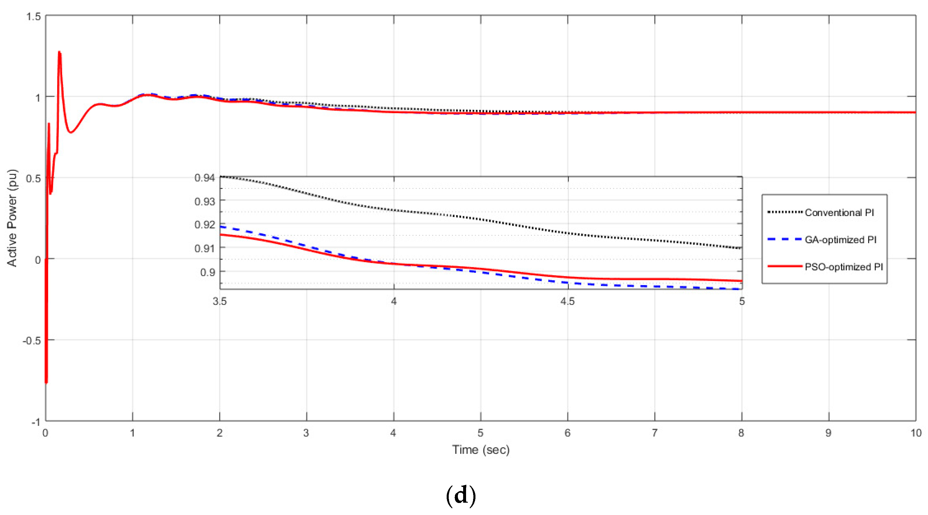
Figure 6 shows the system response in Case 1. The system response is faster using the PSO-optimized controller than using the GA-optimized or conventional controller. By minimizing the settling time of the pitch angle controller response, the pitch angle value of 8.7° for the wind speed of 15 m/s is achieved in a shorter time using the PSO-optimized controller, as depicted in
Figure 6a. Consequently, the generator speed and output power are improved with the optimized controllers, as shown in
Figure 6b,c, respectively, whereas
Figure 6d shows variations in the active power. The PSO-optimized controller stands out in rapidly achieving the steady active power.
6.2. Case 2
When the voltage abruptly changes to 0.5 p.u., it causes oscillation on the DFIG output power. In this case, a fault is introduced, but only for a very small interval at
t = 0.03 s to
t = 0.13 s, which causes transient oscillation, whereas wind speed is kept constant at 15 m/s. Transient oscillations have a significant impact on the dynamic response, and the system response is robust when such events occur. While these faults are associated with the electrical control of the system, the response of the optimized pitch angle controller is fast, as can be seen in
Figure 7a, due to the generator speed error being subjected to optimization. Because the dynamics of the electrical control system are extremely quick to deal with electrical faults and no controlling variable of pitch control is involved, the optimized values of the controller parameters are the same as obtained in Case 1 and as shown in
Table 2.
The optimized model performs better than the conventional model. The error induced in the generator speed settles to a minimum value rapidly in case of the PSO optimized controller, comparatively, as visible from
Figure 7b,c, which shows that the system’s active power precisely follows the reference power line for all the controllers, but the PSO based controller has a better settling response.
Figure 7d shows the active power variations attained by the three controllers.
6.3. Case 3
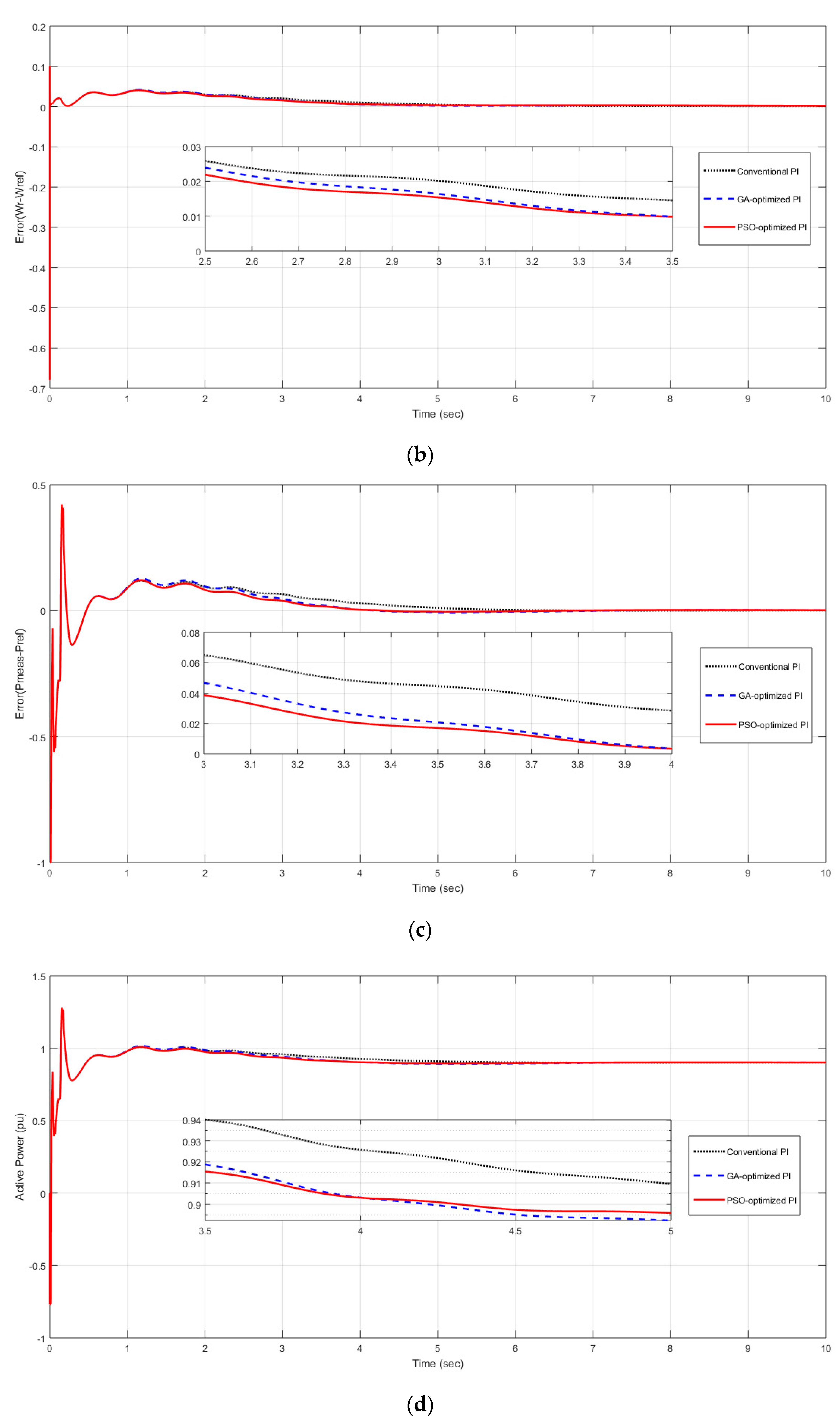
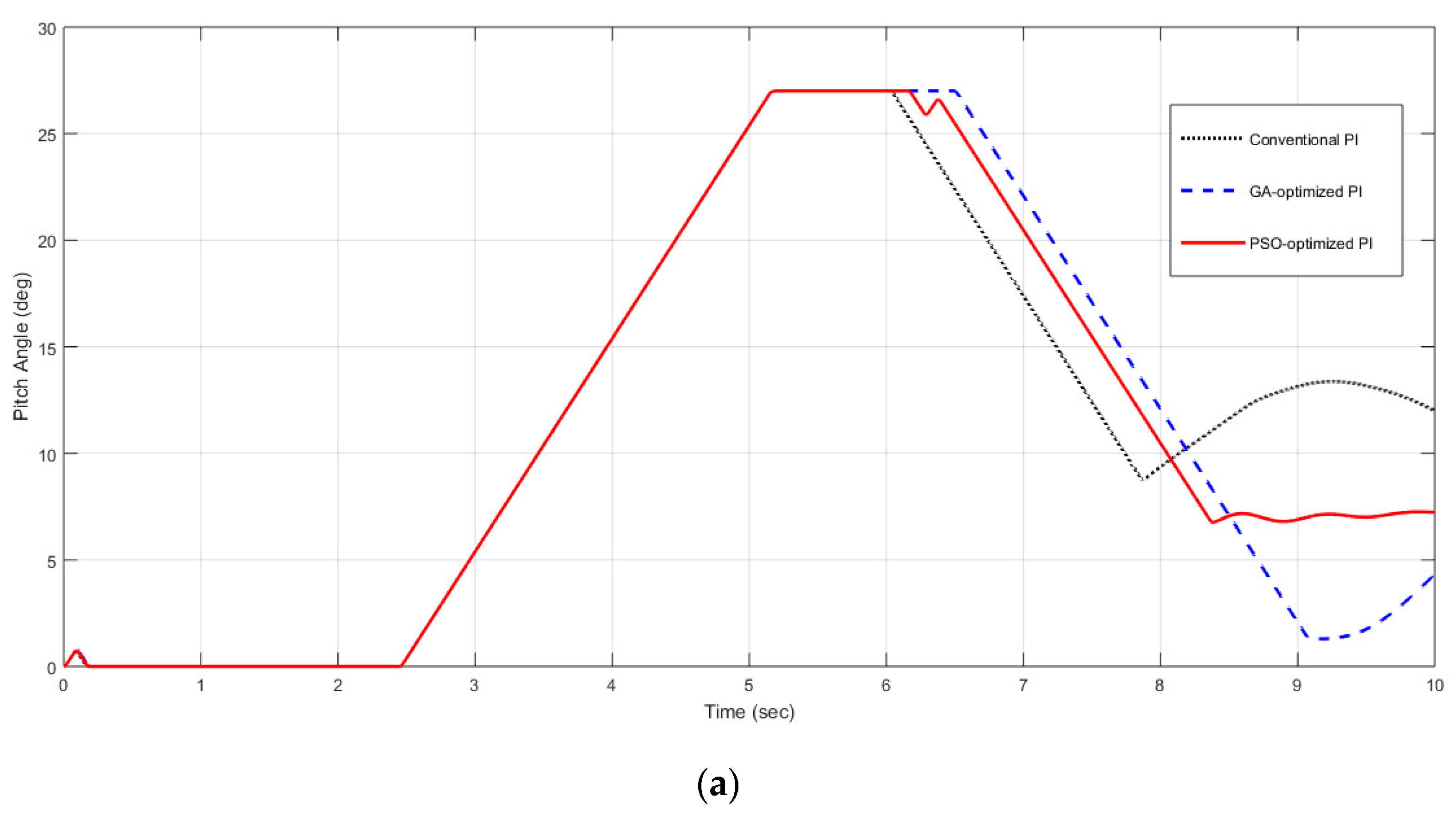
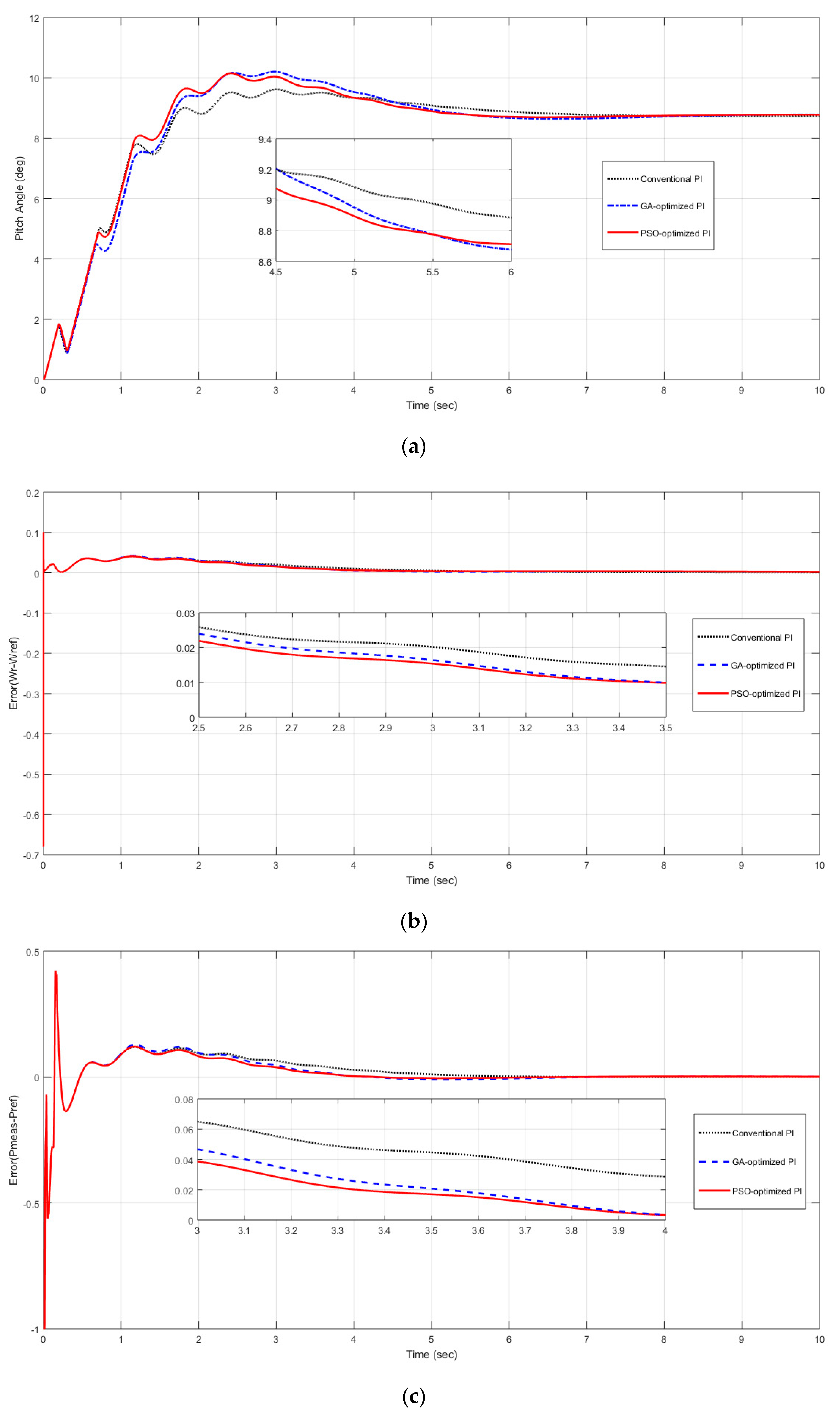
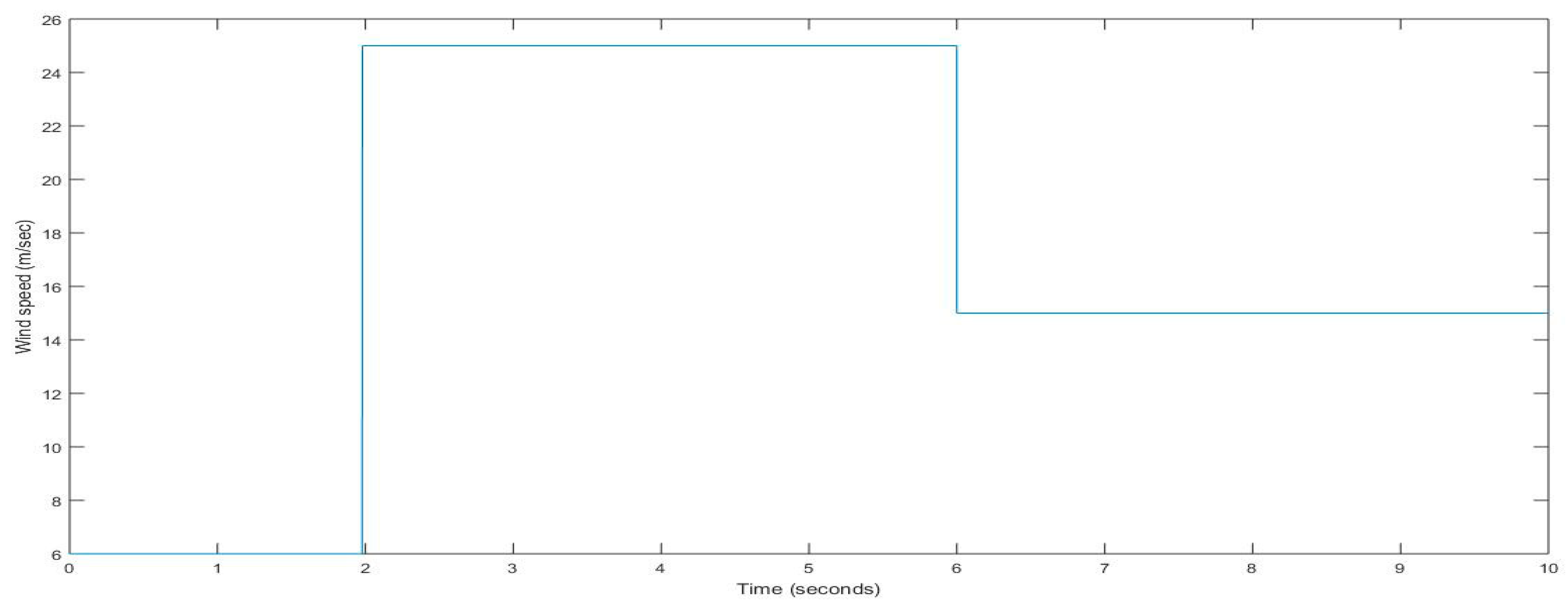
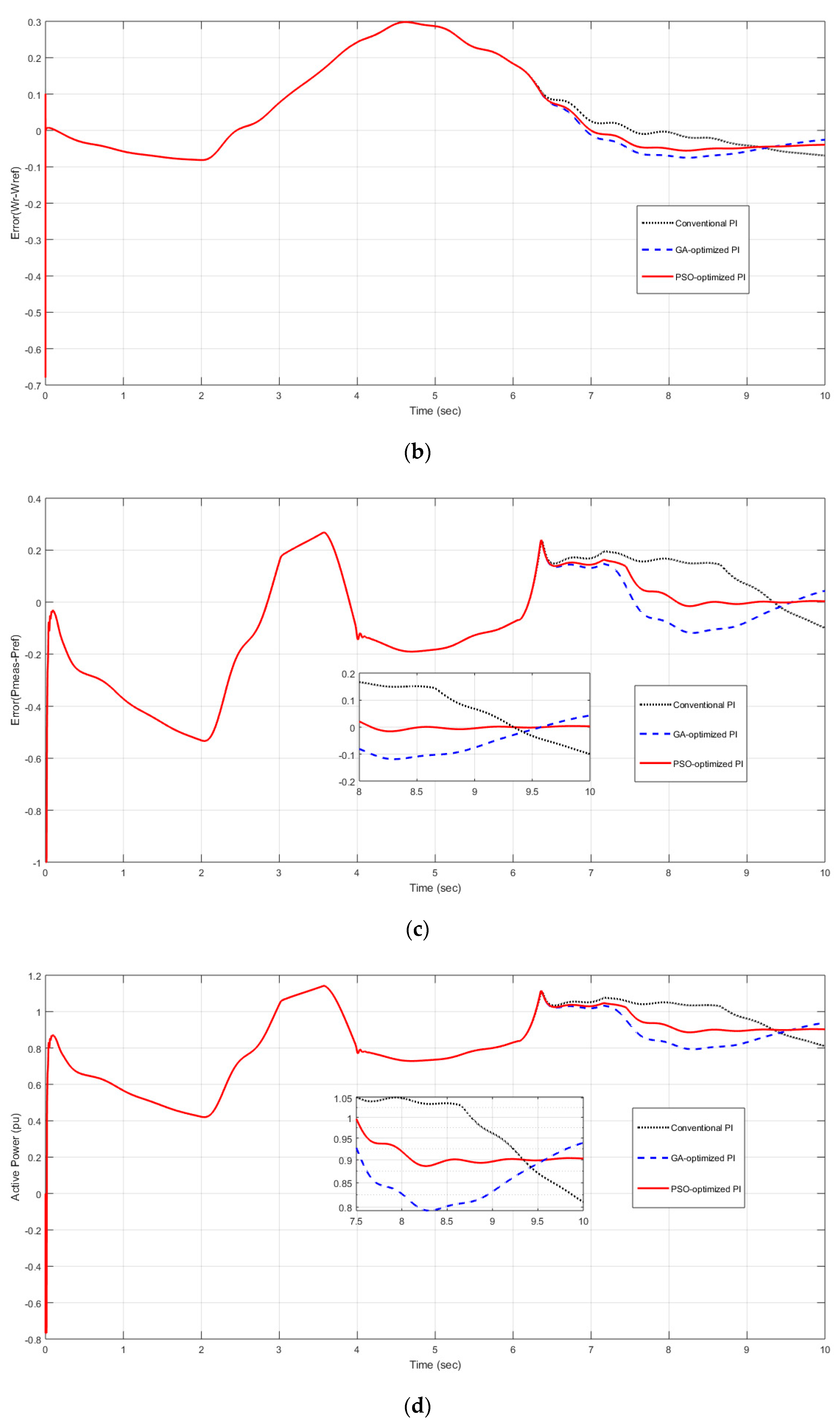
When wind variations are introduced, the controller modifies the blade pitch. The pitch angle controller actuator is rate limited, and there is a time constant associated when translating the controller signal to mechanical output. For fast wind gusts, the controller response is appropriate, but sluggish due to the time constant. In this case, the model inherits the fault from the previous case, causing the initial overshoot. The wind variations are very fast, and hence, the dynamics of conventional and optimized controllers are observed for comparative system response. The wind is varying, for example, from 0 to 2 s, the wind speed is 6 m/s, from 2 to 6 s, the wind speed is 25 m/s, and from 6 to 10 s, the wind is at 15 m/s, as shown in
Figure 8.
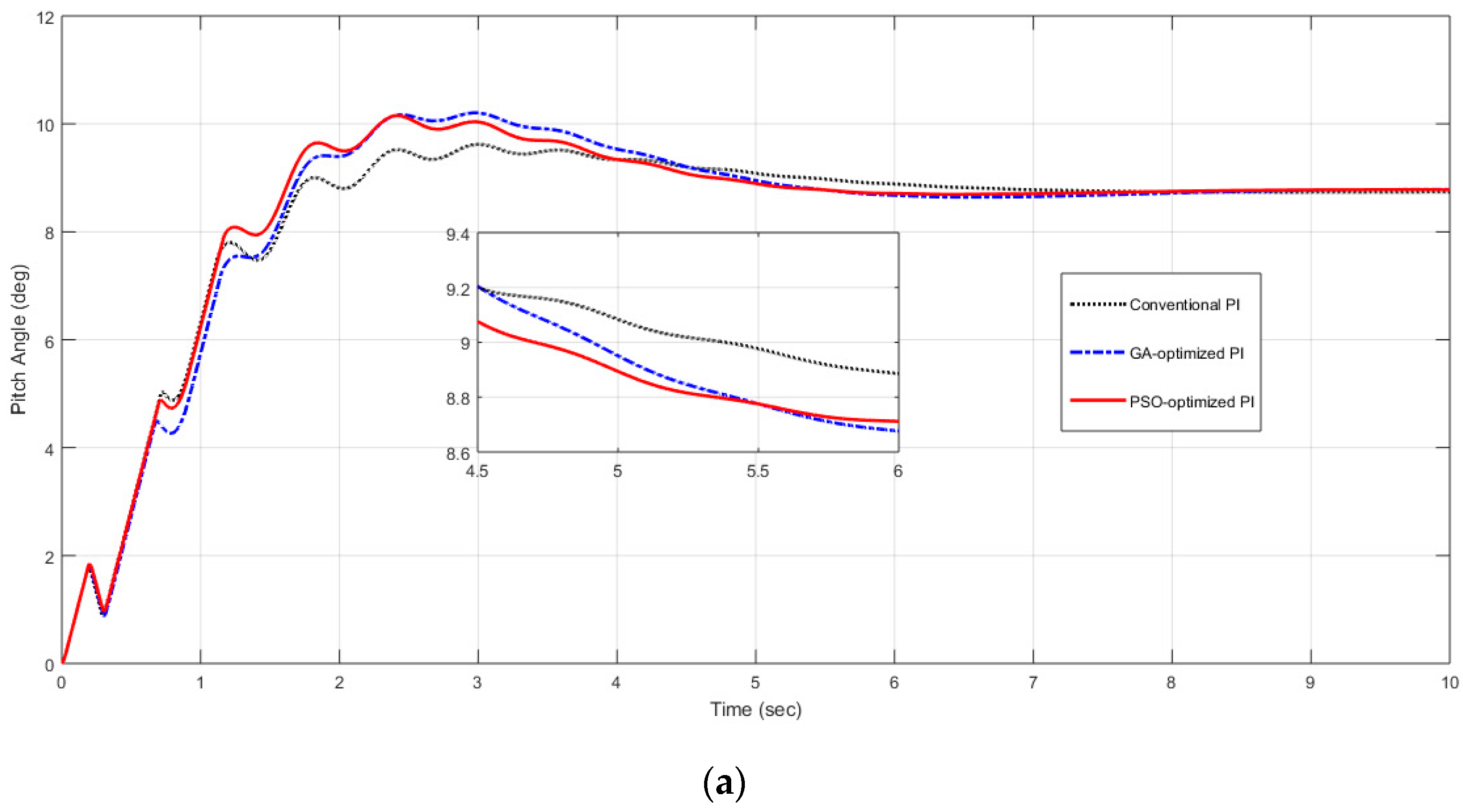
As shown in
Figure 9a, the pitch angle remains zero for lower wind speeds and rises to a maximum value of 27°, when wind speed changes to a much higher value. The pitch angle of 8.7° is achieved when the wind speed changes to nominal value. The dynamic response of the pitch angle controller with fast wind variations is improved with the PSO-optimized model. The PSO-optimized model shows that it controls the output power flow more efficiently than do the GA-optimized model or the original model, as depicted in
Figure 9b–d.
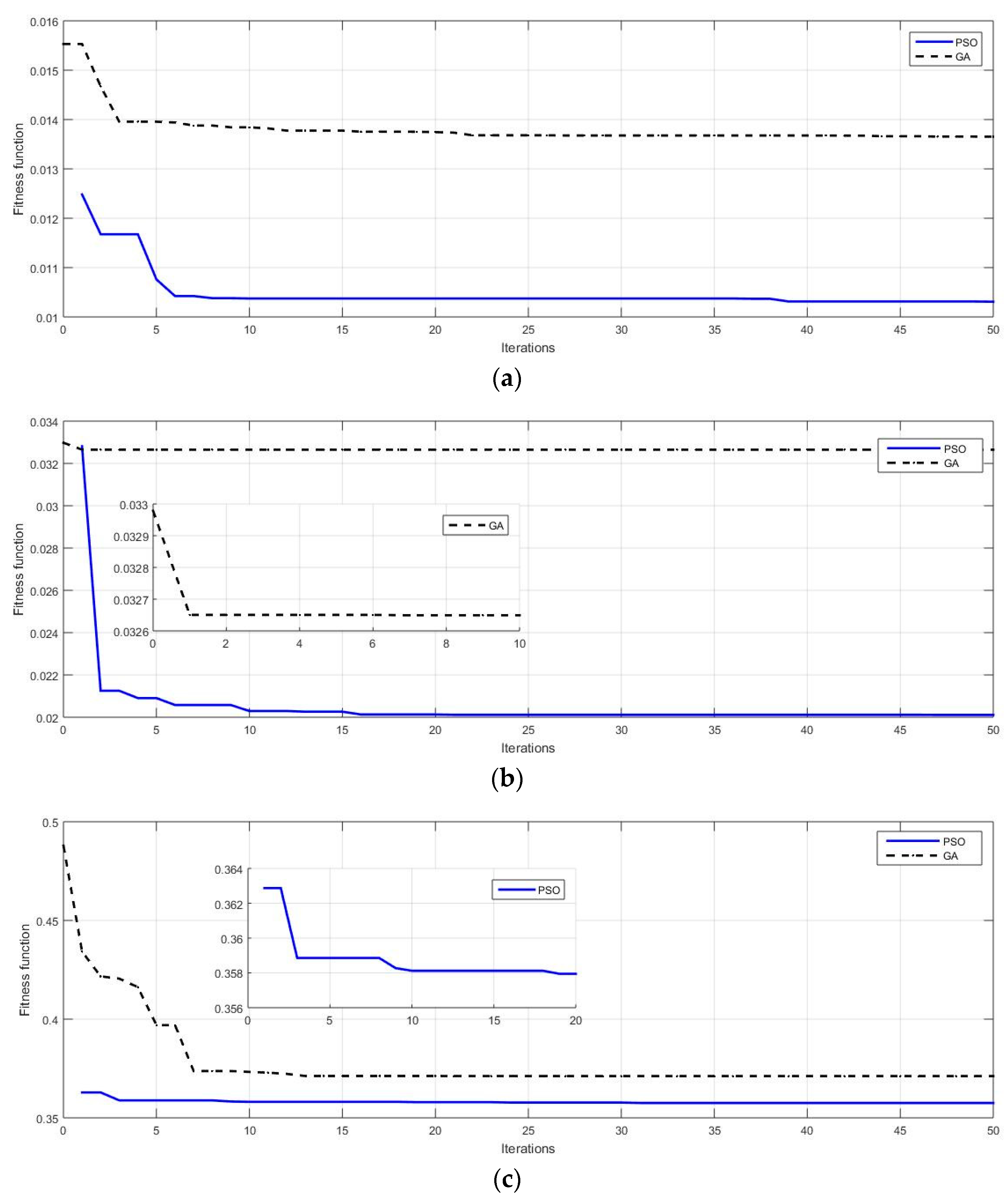
The convergence curves for GA and PSO for all three cases have been shown in
Figure 10a–c, respectively. The convergence curves evaluate the performance of the optimization algorithm. PSO performed better than GA in all three cases and achieved minimum fitness values in each case; this is shown in
Table 2. Hence, more optimal values of controller parameters and better system response are achieved in all cases for the PSO-optimized controller.
The performance criteria defined in
Table 1 are calculated for the error functions
and
and tabulated in
Table 3 for the three cases. It is obvious from
Table 3 that ITSE has minimum values for
, and MAE has minimum values for
. Prior knowledge of best performance criteria in MOO eliminates articulating weightage to each objective during optimization.
Table 2 shows the parameter values for the original system and the system optimized using the GA and the PSO algorithms.
Table 4 shows the optimal values of the objective function defined in (12) for the three cases. For the minimum value of the objective function, the optimization algorithms perform better. The initial values of the function are corresponding to the original values of the controllers’ parameters, as shown in
Table 3. These values are attained by running the objective function as in (12), without optimization, and selecting original controller parameters as optimal.
7. Conclusions
Computational optimization techniques have been used for improving the dynamic response of the pitch angle controller in three different cases. Using PSO and GA, the parameters of the pitch angle controller are optimized.
From the results observed in three different cases, it is concluded that computational optimization is effective in improving the overall response of the system. However, these results are subject to a better implementation of optimization algorithms and a good choice of optimization techniques. PSO is found to be more suitable than GA for this specific application. The results also improved the control of the variables using pitch angle control. The pitch angle controller is more effective in controlling the output power and generator speed during wind variations than during a faulty condition. The response of the controller is improved in all three cases by optimizing the parameter values of the pitch angle controller.
The proposed methodology is evidently very efficient for optimizing parameters in the system design, although it is limited for adaptive control schemes because implementing optimization techniques with this approach requires deep analysis and manual selections for optimal solutions, which contradicts the concept of adaptive control in real time applications.
Author Contributions
Conceptualization, M.A.M.; Data curation, T.A.-H.; Formal analysis, A.K. and T.A.-H.; Funding acquisition, T.A.-H.; Investigation, A.K., A.O. and I.K.; Methodology, M.A.M. and I.K.; Project administration, J.A.; Resources, A.O. and H.K.; Software, A.K., H.K. and A.; Supervision, A. and J.A.; Visualization, I.K.; Writing—original draft, A.K.; Writing—review and editing, A. and J.A. All authors have read and agreed to the published version of the manuscript.
Funding
This research is funded by Computing and Informatics Research Centre (CIRC) Group at School of Science and Technology (Department of Computer Science) in Nottingham Trent University, UK.
Acknowledgments
One of the authors (Harish Kumar) extends his gratitude to the Deanship of Scientific Research at King Khalid University for funding this work through the research groups program under grant number R. G. P. 2/132/42.
Conflicts of Interest
The authors declare no conflict of interest.
Appendix A
This section presents the parameter used for wind turbine and associated components in this simulation.
Table A1,
Table A2,
Table A3,
Table A4,
Table A5,
Table A6, and
Table A7 shows the parameters for wind turbine, drive train, generator, converter, controller, PSO and GA algorithm respectively.
Table A1.
Turbine Data.
| Mechanical output power (W) | 1.5 × 10⁶ |
| Wind speed at Cp (max) (must be b/w 6 m/s and 30 m/s) | 15 |
| Initial wind speed (m/s) | 15 |
Table A2.
Drive Train Data.
Table A2.
Drive Train Data.
| Wind turbine inertia constant: H | 4.32 |
| Shaft spring constant refers to the high-speed shaft (p.u) | 1.11 |
| Shaft mutual damping (p.u) | 1.5 |
| Turbine initial speed (p.u) | 1.2 |
| Initial output torque (p.u) | 0.83 |
Table A3.
Generator data.
Table A3.
Generator data.
| Nominal power, PN (VA) | 1.5 × 10⁶ |
| VLL: [Vstator (rms) Vrotor (rms)] (Volts) | (575, 1975) |
| Frequency (Hz) | 60 |
| Stator [R L] (p.u) | (0.023, 0.18) |
| Rotor [R L] (p.u) | (0.016, 0.16) |
| Magnetizing inductance Lm (p.u) | 2.9 |
| Inertia constant, friction factor, and pair of poles [H F P] | (0.685, 0.01, 3) |
Table A4.
Converter data.
Table A4.
Converter data.
| GSC maximum current (p.u) | 0.8 |
| Grid-side coupling inductor [L, R] (p.u) | (0.3, 0.003) |
| Nominal DC bus voltage (Volts) | 1150 |
| Line filter capacitor (Q = 50) (VAR) | 120 × 103 |
| DC bus capacitor (F) | 10,000 × 10−6 |
Table A5.
Control parameters.
Table A5.
Control parameters.
| DC bus voltage regulator gains [Kp Ki] | (8, 400) |
| GSC current-regulator gains [Kp Ki] | (0.83, 5) |
| Speed regulator gains [Kp Ki] | (3 0, 0.6) |
| RSC regulator gains [Kp Ki] | (0.6, 8) |
| Q and V regulator gains [Ki(VAR) Ki(volt)] | (0.05, 20) |
| Pitch controller gain [Kp] | (150) |
| Maximum pitch angle | 27 |
| The maximum rate of change of the pitch angle (Deg./s) | 10 |
Table A6.
PSO parameters.
Table A6.
PSO parameters.
| 0.9 |
| 2 |
| 2 |
| Population size | 5 |
| Maximum iterations | 50 |
Table A7.
GA parameters.
| Selection | Stochastic |
|---|
| Crossover probability | 0.8 |
| Mutation probability | 0.05 |
| Population size | 5 |
| Generations | 50 |
References
- IRENA. Future of Wind: Deployment, Investment, Technology, Grid Integration and Socio-Economic Aspects (A Global Energy Transformation Paper); International Renewable Energy Agency: Abu Dhabi, United Arab Emirates, 2019. [Google Scholar]
- Mwaniki, J.; Lin, H.; Dai, Z. A Concise Presentation of Doubly Fed Induction Generator Wind Energy Conversion Systems Challenges and Solutions. J. Eng. 2017, 2017, 4015102. [Google Scholar] [CrossRef] [Green Version]
- Muller, S.; Deicke, M.; de Doncker, R.W. Doubly fed induction generator systems for wind turbine. IEEE Ind. Appl. Mag. 2002, 3, 26–33. [Google Scholar] [CrossRef]
- Wu, F.; Ju, P.; Zhang, X.P. Parameter Tuning for Wind Turbine with Doubly Fed Induction Generator Using PSO. In Proceedings of the 2010 Asia-Pacific Power and Energy Engineering Conference, Chengdu, China, 28–31 March 2010; pp. 1–4. [Google Scholar]
- Vidal, P.-E.; Pietrzak-David, M.; Bonnet, F. Mixed control strategy of a doubly fed induction machine. Electr. Eng. 2008, 90, 337–346. [Google Scholar] [CrossRef]
- Peresada, S.; Tilli, A.; Tonielli, A. Power control of a doubly fed induction machine via output feedback. Control. Eng. Pract. 2004, 12, 41–57. [Google Scholar] [CrossRef]
- Peresada, S.; Tilli, A.; Tonielli, A. Indirect stator flux-oriented output feedback control of a doubly fed induction machine. IEEE Trans. Control. Syst. Technol. 2003, 11, 875–888. [Google Scholar] [CrossRef]
- Cardenas, R.; Pena, R.; Proboste, J.; Asher, G.; Clare, J. MRAS observer for sensorless control of standalone doubly fed induction generators. IEEE Trans. Energy Convers. 2005, 20, 710–718. [Google Scholar] [CrossRef]
- Daili, Y.; Gaubert, J.P.; Rahmani, L. Implementation of a new maximum power point tracking control strategy for small wind energy conversion systems without mechanical sensors. Energy Convers. Manag. 2015, 97, 298–306. [Google Scholar] [CrossRef]
- Yang, B.; Zhang, X.; Yu, T.; Shu, H.; Fang, Z. Grouped grey wolf optimizer for maximum power point tracking of doubly-fed induction generator-based wind turbine. Energy Convers. Manag. 2017, 133, 427–443. [Google Scholar] [CrossRef]
- D
e Prada Gil, M.; Sumper, A.; Gomis-Bellmunt, O. Modeling and control of a pitch-controlled variable-speed wind turbine driven by a DFIG with frequency control support in PSS/E. In Proceedings of the 2012 IEEE Power Electronics and Machines in Wind Applications, Denver, CO, USA, 16–18 July 2012; pp. 1–8. [Google Scholar]
- Hosseini, E.; Shahgholian, G. Output power levelling for DFIG wind turbine system using intelligent pitch angle control. Automatika 2017, 58, 363–374. [Google Scholar] [CrossRef]
- Yang, L.; Yang, G.Y.; Xu, Z.; Dong, Z.Y.; Wong, K.P.; Ma, X. Optimal controller design of a doubly-fed induction generator wind turbine system for small signal stability enhancement, in IET Generation. Transm. Distrib. 2010, 4, 579–597. [Google Scholar] [CrossRef]
- Lin, W.M.; Hong, C.M.; Ou, T.C.; Chiu, T.M. Hybrid intelligent control of PMSG wind generation system using pitch angle control with RBFN. Energy Convers. Manag. 2011, 52, 1244–1251. [Google Scholar] [CrossRef]
- Marler, R.T.; Arora, J.S. The weighted sum method for multi-objective optimization: New insights. Struct. Multidisc. Optim. 2010, 41, 853–862. [Google Scholar] [CrossRef]
- Nagaria, D.; Pillai, N.; Gupta, H.O. Particle swarm optimzitation approach for controller design in WECS equipped with DFIG. J. Electr. Syst. 2010, 6, 1–17. [Google Scholar]
- Behera, S.; Subudhi, B.; Pati, B.B. Design of PI controller in pitch control of wind turbine: A comparison of PSO and PS algorithm. Int. J. Renew. Energy Res. 2016, 6, 271–281. [Google Scholar]
- Senjyu, T.; Sakamoto, R.; Urasaki, N.; Funabashi, T.; Fujita, H.; Sekine, H. Output power leveling of wind turbine generator for all operating regions by pitch angle control. IEEE Trans. Energy Convers 2006, 21, 467–475. [Google Scholar] [CrossRef]
- Zhang, J.; Cheng, M.; Chen, Z.; Fu, X. Pitch angle control for variable speed wind turbines. In Proceedings of the 2008 Third International Conference on Electric Utility Deregulation and Restructuring and Power Technologies, Nanjing, China, 6–9 April 2008; pp. 2691–2696. [Google Scholar]
- Chowdhury, M.A.; Hosseinzadeh, N.; Shen, W.X. Smoothing wind power fluctuations by fuzzy logic pitch angle controller. Renew. Energy 2012, 38, 224–233. [Google Scholar] [CrossRef]
- Gnanamalar, S.S.R. Performance analysis of conventional pitch angle controllers for DFIG. Int. J. Pure Appl. Math. 2017, 116, 1–9. [Google Scholar]
- Aldair, M.D. Pitch angle control design of wind turbine using fuzzy-art network. J. Eng. Dev. 2014, 18, 39–51. [Google Scholar]
- Miller, N.W.; Sanchez-Gasca, J.J.; Price, W.W.; Delmerico, R.W. Dynamic modeling of GE 1.5 and 3.6 MW wind turbine-generators for stability simulations. In Proceedings of the 2003 IEEE Power Engineering Society General Meeting, Toronto, ON, Canada, 13–17 July 2003; Volume 3, pp. 1977–1983. [Google Scholar]
- Galdi, V.; Piccolo, A.; Siano, P. Designing an adaptive fuzzy controller for maximum wind energy extraction. IEEE Trans. Energy Convers. 2008, 23, 559–569. [Google Scholar] [CrossRef]
- Yang, X.; Koziel, S.; Liefsson, L. Computational optimization, modelling and simulation: Recent trends and challenges. Procedia Comput. Sci. 2013, 18, 855–860. [Google Scholar] [CrossRef] [Green Version]
- Kennedy, J.; Eberhart, R. Particle swarm optimization. In Proceedings of the ICNN’95—International Conference on Neural Networks, Perth, Australia, 27 November–1 December 1995; pp. 1942–1948. [Google Scholar]
- Qiao, W.; Venayagamoorthy, G.K.; Harley, R.G. Design of Optimal PI Controllers for Doubly Fed Induction Generators Driven by Wind Turbines Using Particle Swarm Optimization. In Proceedings of the 2006 IEEE International Joint Conference on Neural Network Proceedings, Vancouver, BC, Canada, 16–21 July 2006; pp. 1982–1987. [Google Scholar]
- Pham, H. A New Criterion for Model Selection. Mathematics 2019, 7, 1215. [Google Scholar] [CrossRef] [Green Version]
| Publisher’s Note: MDPI stays neutral with regard to jurisdictional claims in published maps and institutional affiliations. |
© 2022 by the authors. Licensee MDPI, Basel, Switzerland. This article is an open access article distributed under the terms and conditions of the Creative Commons Attribution (CC BY) license (https://creativecommons.org/licenses/by/4.0/).


 ,
, 


