A Study on Performance Metrics for Anomaly Detection Based on Industrial Control System Operation Data

Abstract

Recently, OT (operational technology) networks of industrial control systems have been combined with IT networks. Therefore, OT networks have inherited the vulnerabilities and attack paths existing in IT networks. Consequently, attacks on industrial control systems are increasing, and research on technologies combined with artificial intelligence for detecting attacks is active. Current research focuses on detecting attacks and improving the detection accuracy. Few studies exist on metrics that interpret anomaly detection results. Different analysis metrics are required depending on the characteristics of the industrial control system data used for anomaly detection and the type of attack they contain. We focused on the fact that industrial control system data are time series data. The accuracy and F1-score are used as metrics for interpreting anomaly detection results. However, these metrics are not suitable for evaluating anomaly detection in time series data. Because it is not possible to accurately determine the start and end of an attack, range-based performance metrics must be used. Therefore, in this study, when evaluating anomaly detection performed on time series data, we propose a range-based performance metric with an improved algorithm. The previously studied range-based performance metric time-series aware precision and recall (TaPR) evaluated all attacks equally. In this study, improved performance metrics were studied by deriving ambiguous instances according to the characteristics of each attack and redefining the algorithm of the TaPR metric. This study provides accurate assessments when performing anomaly detection on time series data and allows predictions to be evaluated based on the characteristics of the attack.

1. Introduction

Recently, attacks targeting industrial control systems have been increasing. This is because OT networks, which were more closed off in the past, have been combined with IT networks, and the number of devices communicating with the outside has increased [1,2]. Therefore, OT networks have inherited the vulnerabilities and attack paths and vectors that exist in IT networks. Notably, because various industrial control systems comprise national infrastructure, the scale of damage caused by an attack is significantly large. Therefore, research on protection and detection methods is being actively conducted. In the past, systems such as firewalls, IDSs, and IPSs were introduced to protect and detect external attacks. However, recently, attention has shifted toward solutions involving artificial intelligence, a core element of the Fourth Industrial Revolution [3,4]. Most studies focus on using machine learning, which uses deep learning to train testbed-based data to improve accuracy and detect more anomalies. However, research on how to interpret the results of anomaly detection is limited. An appropriate interpretation must be made according to the characteristics of the data applied to the anomaly detection and the type of attack they contain.

The data extracted from industrial control systems are characteristically time series data. To perform and evaluate anomaly detection on time series data, non-traditional performance metrics are needed. In many cases, standard point-based metrics are used when evaluating detections. However, standard point-based metrics cannot accurately evaluate anomaly detection on time series data. Standard point-based metrics give higher scores to detect longer anomalies. However, it is important to detect various attacks in industrial control systems. Therefore, point-based metrics are not appropriate because they give higher scores to the method of detecting multiple attacks and the method of detecting long attacks, whichever method that may be. In addition, abnormal behavior that occurs in industrial control systems often progresses slowly over a long period of time. Therefore, it is difficult to clearly grasp the start and end points of an attack. It is necessary to evaluate the result of anomaly detection in consideration of its characteristics.

The purpose of our research is to evaluate the performance of anomaly detection and suggest directions for further improving the performance metrics, using performance metrics that characterize the data. We overwrote the ambiguous section of the time-series aware precision and recall (TaPR) metric [5], which is a range-based performance metric. TaPR consists of a detection score and a partial score. At this time, the partial score is given in consideration of the feature that it is difficult to grasp the start and end points of the attack. We looked at this ambiguous section of the algorithm and figured out that we could apply the same percentage to all anomalous behaviors to derive the ambiguous section. The attack duration section is from the moment the attacker starts attacking the system to the moment it stops. However, the sections in which the system is actually affected are different. Assuming the system was attacked by an attacker while it was operating normally, the physical operating values will begin to change over time. Then, the moment the operator sets the threshold value, the real affected section begins. The real affected section is not the moment when the attacker finishes the attack, but the moment when the physical action value reaches below the threshold value. Therefore, this section is not directly affected by the attacker, but it means that the attack remains and affects the system. The duration of the attack and the real affected section are different for each attack. We would like to focus on this part and define ambiguous sections according to the characteristics of the attack.

In summary, our contributions include the following:

• We create training models and perform anomaly detection using operation datasets derived from real industrial control systems;
• We propose a range-based metric suitable for evaluating anomaly detection against time series data;
• We redefine the algorithm for the ambiguous section of TaPR in consideration of the characteristics of the attack.

This paper is structured as follows. In Section 2, we discuss industrial control systems and the data in the networks and operating systems of the industrial control system datasets that have been published thus far. Section 2 also describes the standard and time-series-based performance metrics typically used to describe the proposed anomaly detection assessment of performance metrics. After that, we analyze the operational data to determine which performance index to use for the anomaly detection research. Section 3 proposes an improved algorithm for the time-series aware precision and recall (TaPR) metric, a time-series-based performance metric. We redefine the algorithm of the ambiguous section of the TaPR metric using the upper control line (UCL) and lower control line (LCL), which are concepts of statistical process control (SPC). In Section 4, we perform and analyze anomaly detection in our operational database using deep learning. Additionally, the redefined algorithm proposed in Section 3 is applied to the case study. Finally, Section 5 draws conclusions and presents future research directions.

2. Related Works

2.1. Industrial Control System Structure and Security Requirements

A control system is a device that manages, commands, directs, and regulates the operation of other devices or systems. It is a system that can affect the real world, and that connects cyber and physical processes. According to the IEC 62443 standard, an industrial control system is a collection of processes, personnel, hardware, and software that affects, or can affect, the safety, security, and reliable operation of industrial processes. The industrial control system structure is described in reference to the PERA (Purdue Enterprise Reference Architecture) model [6] in Figure 1, one of the reference architectures demonstrating industrial control networks. The PERA model is a reference model easily understood by dividing devices and equipment into layers [7,8]. The PERA model is primarily divided into a safety zone, an industrial zone from levels 0 to 3, and an enterprise zone from levels 4 to 5.

Figure 1. Structure of the PERA (Purdue Enterprise Reference Architecture) model.

The safety zone is where the safety instrumentation system, responsible for the safe operation of the industrial control system, is located. The industrial zone is called OT (operation technology) and includes the cell/area zone containing levels 0, 1, and 2, as well as level 3, which serves as a control center that integrates and manages multiple cells/areas. Level 0 is the process area, consisting of I/O devices that recognize and manipulate physical processes, including sensors that measure temperature, humidity, pressure, etc., and actuators that control equipment according to the commands from the controller. Level 1 is the basic control area, primarily composed of a manufacturing process controller interacting with level 0 devices and operated by a PLC (programmable logic controller) and VFD (variable frequency drive). Level 2 is the supervision and control area, where an operator HMI (human–machine interface) and alarm systems that supervise and control operations are operated [9].

Level 3 is the field operation management area comprising an application server that integrates the monitoring and control of physical on-site processes, an engineer workstation that configures and controls the overall hardware of the industrial control system, an HMI, a domain controller, and a historian server that primarily uses a real-time database. This level is an essential zone because there are applications, devices, and controllers crucial for monitoring and controlling the industrial control system. An antivirus or patch management server operates in this area. The enterprise zone includes levels 4 and 5 and refers to an environment where the production management system, manufacturing execution system (MES), process monitoring, general IT system application, enterprise resource planning (ERP) system, and e-mail server are installed [9].

Industrial control systems introduced and operated in the national infrastructure are rapidly becoming intelligent and digitized. In addition, the increase in connectivity be-tween heterogeneous devices in various environments owing to the Fourth Industrial Revolution triggers the expansion of the attack surface of the existing IT environment security threats to the OT environment, leading to more diverse security threats than before [10].

According to the international standard IEC 62443, a standard that defines regulations and requirements exists. IEC 62443-1-1 describes seven functional requirements (FR), such as the definition of the control system capability security level and component requirements [11]. This study focused on the timely event response and resource availability among the seven requirements of IEC 62443-4-2 [12]. The two requirements focus on a control system’s safe monitoring and operation. Therefore, monitoring the operation data in the industrial control system in real time and performing anomaly detection are necessary. In the past, behavior-based IDSs/IPSs were used, but recently, anomaly detection has also begun to use neural network algorithms.

2.2. Datasets

The data extracted from industrial control systems can be divided into network traffic and operating system datasets. Table 1 shows the operating system datasets, where five types were investigated. The operating system conducts a scenario-based attack through the attack point.

Table 1. Industrial control system operation dataset list.

	Name	Proposed	Attack Points	Year
[13]	ICS Cyber Attack Datasets	Tommy Morris	32	2015
[14]	BATADAL	iTrust	14	2017
[15]	WADI	iTrust	15	2019
[16]	SWaT Datasets	iTrust	41	2015
[17,18]	HAI Datasets	NSR	50	2020

The first dataset is from the ICS Cyber Attack Datasets [13], consisting of datasets for five processes: power systems, gas pipelines, gas pipelines and water storage tanks, improved gas pipelines, and energy management systems. The second dataset is BATADAL [14], a dataset from a contest aimed at generating an attack detection algorithm, based on a water distribution system, and consisting of three datasets, two for training data and one for validation. Training data #1 are normal data collected for one year, and training data #2 are data collected for 6 months and consist of normal data and attacked data. Data for verification are unlabeled data collected for 4 months. The third dataset is WADI [15], which was generated from multiple testbeds extended from the SWaT testbed. The drainage testbed simulates water demand and consumption over time. It collects steady-state data for 14 days and contains attacks for 2 days.

The fourth dataset is SWaT [16], which was collected from the testbed of a water treatment system. It contains the physical devices that make up each stage of the water treatment system, and eight versions through seven renewals exist thus far. The fifth dataset is HAI [17], which comprises data collected from a water treatment process system. It consists of three physical systems, namely, GE’s turbine, Emerson’s boiler, and FESTO’s water treatment system, and a dSPACE HIL simulator. The variables measured and controlled by the control system were collected at 1 s intervals at 78 points. Currently, versions 20.07 [18] and 21.03 exist, and the renewed 21.03 version adds attack and collection points.

2.3. Performance Metrics for Anomaly Detection

Performance metrics for anomaly detection evaluation can be divided into point- and range-based methods, as shown in Figure 2. In point-based methods, only abnormal and normal answer labels are correct, and points are given if the answer is the same. In contrast, range-based methods not only divide into abnormal and normal labels but also assign different scores according to performance metrics. This allows the evaluator to assign different weights to give different scores.

Figure 2. Performance metric tree for anomaly detection evaluation.

2.3.1. Standard Metric

The standard metric refers to a point-based performance index and a function con-structed using items of a confusion matrix. The function uses accuracy and often considers precision and recall as well. There are the F1-score using precision and recall, the ROC curve (receiver operating characteristic curve) using true and false positive rates, and the AUC (area under the curve) indicating the bottom area of the ROC curve.

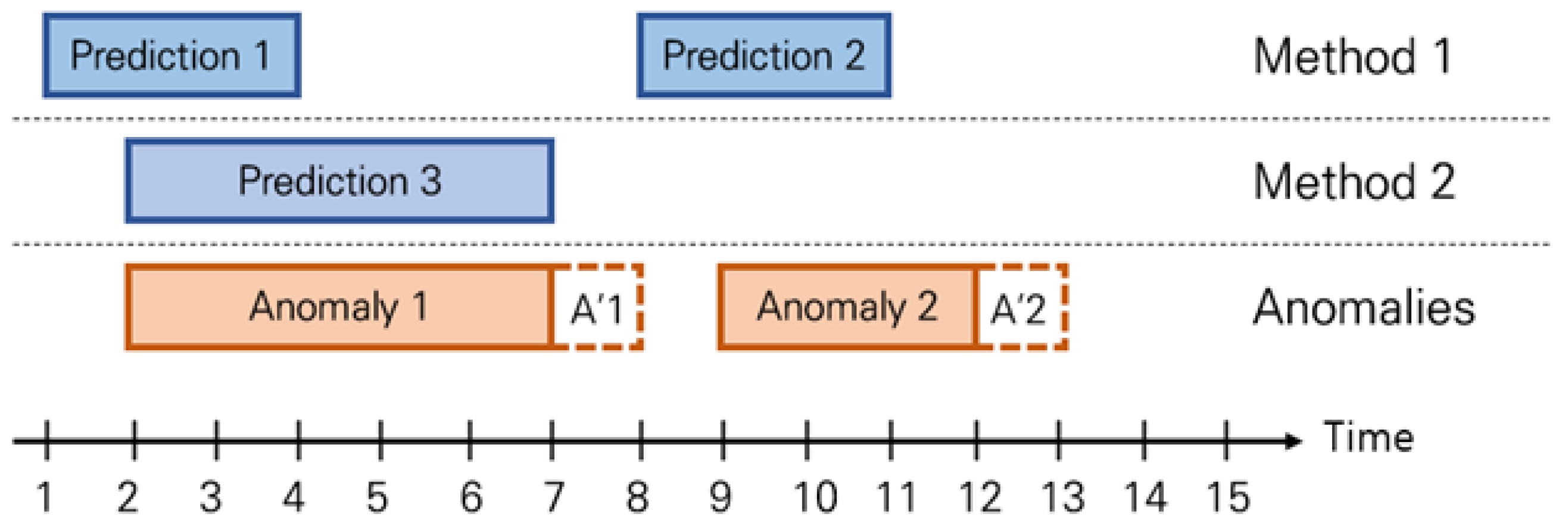
2.3.2. Range-Based Recall and Precision

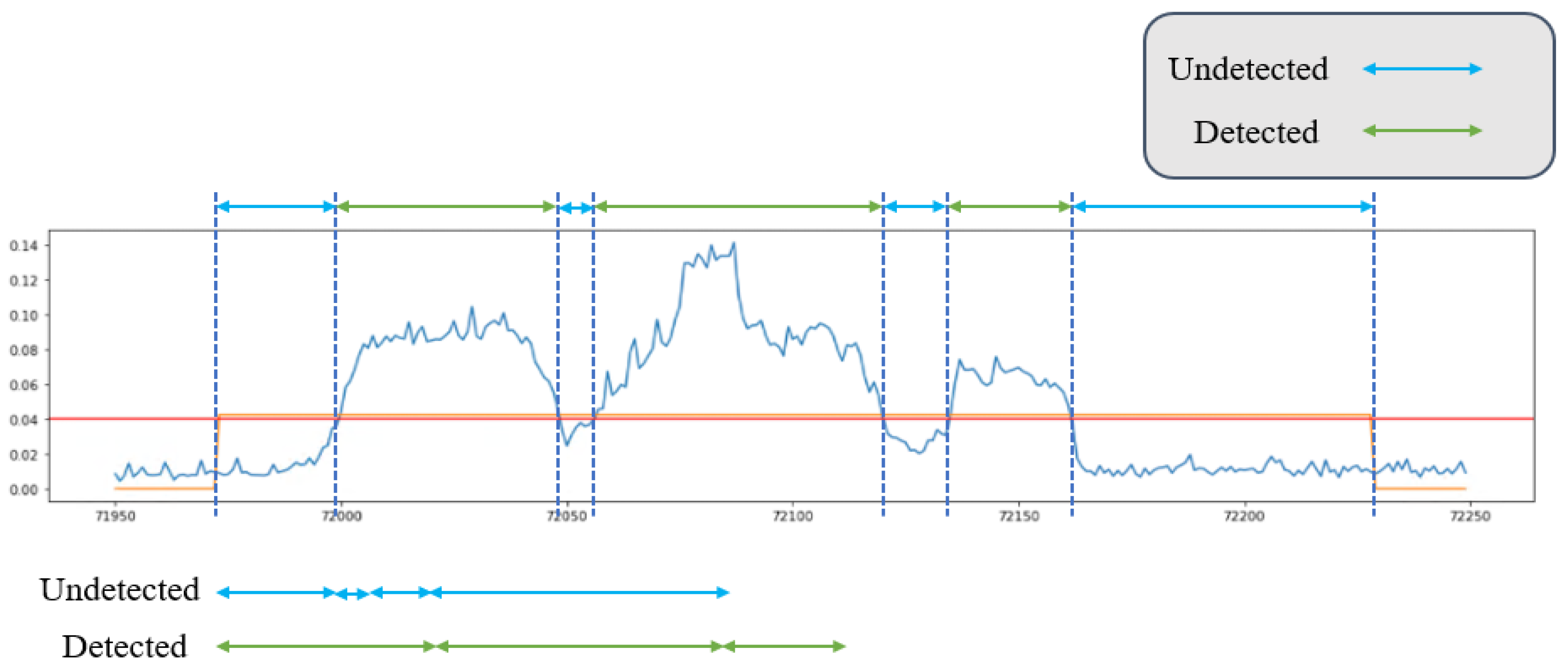
Anomaly detection is defined as a range-based anomaly caused by an atypical event; therefore, using a point-based performance evaluation index is inappropriate for this [19]. Therefore, range-based recall (RR) and precision (RP), which are range-based performance indexes, were used. Recall receives a score if the abnormality is sufficiently identified and a penalty if not. However, because time series data are expressible as a range, recall is an inappropriate performance evaluation index.

2.3.3. TaPR

TaPR was proposed as a performance index suitable for evaluating anomaly detection methods in time series data with time-series aware precision and recall [5]. TaPR consists of a detection score indicating the number of anomalies detected and a subscore indicating how accurately each anomaly was detected. TaPR presents two problems in the existing performance metrics: a method that detects only long anomalies receives a high score; the ambiguity of whether the value derived from the process of returning to the normal value within the physical process is affected by the attack being regarded as normal or abnormal.

Figure 3 presents the problem of giving a high score to a method that detects only long anomalies. Method 1 performed anomaly detection with predictions 1 and 2, and method 2 with prediction 3. The actual anomaly occurred in anomalies 1 and 2 in time units 2 to 8 and 9 to 13 on the time axis. Table 2 shows the precision and recall for methods 1 and 2.

Figure 3. Anomaly detection case to explain problems with existing performance metrics.

Table 2. Precision and recall for methods 1 and 2.

Method	Precision	Recall
1	0.67	0.50
2	1.00	0.625

Method 1 detected all anomalies but had lower precision and recall values than method 2, which detected only one long anomaly. If abnormality 2 is an attack that can have a fatal effect on the internals of the industrial control system, method 1 outperforms method 2 in abnormality detection.

We describe the second problem, the ambiguity, in reference to Figure 4. In Figure 4, the X-axis represents the time, and the Y-axis represents the physical operating values of internal system devices. During normal operation, an attacker carries out an attack, and consequently, the physical operating value exceeds the threshold and reaches a value determined as abnormal. Once the attack ends, section (a) outlines the ambiguous section while returning to the normal value. Section (a) is the process of returning to normal because it is not directly affected by the attacker, but the influence remains. In addition, half of section (a) exceeds the threshold and may be regarded as abnormal, and the other half may be determined as normal because it exceeds the threshold.

Figure 4. Example of an ambiguous section of the TaPR performance metric.

The performance metric derived from these two problems is TaPR. TaPR consists of a detection score and a partial score. The detection score indicates the number of detected anomalies, and the partial score indicates how accurately each anomaly is detected. TaPR emphasizes the importance of the number of anomalies detected through the sum of these two scores. In addition, although the value of ‘normal’ is shown among the sections owing to external influences, this section (a) being ‘abnormal’ is highly likely; thus, if this section is predicted as ‘abnormal’, the subsequent scoring is given. TaP and TaR are calculated as the sum of the detection score (TaP_d, TaR_d) and the portion score (TaP_p, TaR_p). The ambiguous instances used in the portion score are denoted as $a^{\prime }$ and the number of ambiguous instances is denoted as $\delta$ [5] in Table 3.

Table 3. Factors and formulas constituting the performance metrics TaP and TaR.

Factor	Description	Formula
$\alpha$	A set of instances	$a=\left\{ t, t+1, \cdots ,t+l-1 \right\}$
$l$	The number of instances	$\left| a \right|$
$\mathsf{A}$	A set of anomalies	$A=\left\{ a_1, a_2, \cdots ,a_n \right\}$
n	The number of anomalies	-
$\rho$	The suspicious instances	$\rho =\left\{ t\prime , t\prime +1, \cdots ,t\prime +l-1 \right\}$
$\mathsf{{\rm P}}$	A set of predictions	$\mathsf{{\rm P}}=\left\{ {\rho }_1, {\rho }_2, \cdots ,{\rho }_n \right\}$
m	The number of predictions	-
$a\prime$	The ambiguous instances	$a\prime =\left\{ t+1, t+l+1, \cdots ,t+l+\delta +1 \right\}$
$\delta$	The number of ambiguous instances	-
$A\prime$	A set of ambiguous instances	$A\prime =\left\{ a{\prime }_1, a{\prime }_2, \cdots ,a{\prime }_n \right\}$

2.4. Requirements for Performance Metrics

To apply the anomaly detection evaluation method to time series operation data, the following conditions are required for performance metrics:

• The highest score is not given to the method of detecting long-length anomalies.
• Scores are given to cases that detect various anomalies.
• Scores are given to cases that detect proactive signs.
• When an external influence such as an attack is received, the threshold value that separates normal and abnormal is exceeded, and the external influence ends; the value showing abnormality has a score for the case in which it returns to normal.
• A detection score is given according to the characteristics of the attack.

Supplementing the explanation of No. 4 are cases in which the external influence is applied but the boundary value is not exceeded yet, and the external influence is over, but the threshold value is not exceeded. Determining this section only as abnormal and normal is difficult.

Table 4 summarizes papers that performed anomaly detection on the ICS operation dataset and evaluated performance metrics. It is indicated whether the performance metrics used in the papers are point-based or range-based. The authors of [20] conducted an anomaly detection study on the SWaT dataset. SWaT’s attack types consist of single-stage single-point, single-stage multipoint, multistage single-point, and multistage multipoint attacks. Among them, the problem was that there was no research to detect multi-step attacks, and the attacked variables could not be identified. The model used for anomaly detection was the genetic algorithm (GA). To improve detection performance, exponentially weighted moving average smoothing, the mean p-powered error measure, individual error weights for each tag value, and disjoint prediction windows were adjusted. Then, the NAB performance metric was used to evaluate the prediction of anomaly detection. The authors of [21] proposed a deep learning-based anomaly detection method using the Seq-to-Seq model. The study was conducted on the SWaT dataset, and by using the Seq-to-Seq model, it can be said that the encoding–decoding method is suitable for time series operational data. Anomaly detection prediction consists of three steps. In the first stage, the model predicts the sensor and actuator values, and in the second stage, the difference between the predicted data and the actual data is calculated. In the last step, if the difference calculated in step 2 is greater than the set value, it is regarded as abnormal, and a warning is sent. After that, cases in which false negative attacks were not detected and false positives are analyzed. The authors of [22] performed anomaly detection on the SWaT dataset through five machine learning algorithms. SVM, random forest, and KNN were used as supervised learning algorithms, and one-class SVM (OCSVM) and an autoencoder (AE) were used as unsupervised learning algorithms. As an anomaly detection performance evaluation index, values derived from the accuracy and F1-score were compared. On average, supervised learning using data labeling performed better than unsupervised learning, and random forest showed the best performance among the supervised learning algorithms. The authors of [23] studied an intrusion detection mechanism using physical operational data. The method that can be integrated into the network intrusion detection system (NIDS) and the ICS system security were improved. Using operational data, it is easy to detect anomalies in the section without interfering with the communication of each level section. Anomalies were detected using three machine learning models for the HAI 20.03 dataset. The data imbalance problem was solved using the Synthetic Minority Over-sampling Technique (SMOTE). The stratified shuffle split (SSS) method was used for training dataset separation. As a machine learning model, KNN, a decision tree, and a random forest algorithm were used to build the model. Random forest showed the best performance using precision, recall, F1-score, and AUC as performance metrics. The authors of [24] performed anomaly detection based on a stacked autoencoder (SAE) and deep support vector data description (deep SVDD). HAI version 20.03 was used as operational data. Data preprocessing was performed through data scaling, and a model was created through the SAE and deep SVDD. Single event anomaly detection was performed by comparing the accuracies by setting the threshold with the highest accuracy.

Table 4. List of papers researching anomaly detection targeting ICS operation data. (O: Satisfy a requirement, X: Not satisfy a requirement).

	Performance Metrics	Req.1	Req.2	Req.3	Req.4	Req.5	Refs.
Point-based	Confusion Matrix	X	X	X	X	X	[20,21,22,23,24]
	Specificity	X	X	X	X	X
	Recall	X	X	X	X	X
	Precision	X	X	X	X	X
	Accuracy	X	X	X	X	X
Range-based	Ranged-Based Recall and Precision	O	O	X	O	X	[5,19]
	Time-Series Aware Precision and Recall	O	O	O	O	X

Table 4 shows the results of whether the performance metrics presented in Figure 2 satisfy the relevant items. The point-based performance metrics do not satisfy all the conditions. In addition, a study evaluating anomaly detection based on point-based performance metrics is presented. There were papers that studied the range-based performance metrics themselves, but there was no study of anomaly detection using them as performance metrics. Among the range-based performance metrics, RR and RP do not satisfy conditions 3 and 5, and TaPR does not satisfy condition 5. Therefore, in Section 3, we propose performance metrics that satisfy all the conditions by improving the TaPR metric. Moreover, the existing research performed anomaly detection targeting industrial control system time series data but evaluated it using performance metrics in a point-based method. In this paper, the results are derived from the performance metrics of the point-based method and the range-based method. We then compare the results to discuss which method is more suitable for evaluating anomaly detection targeting time series data.

3. Proposed Performance Metrics

In this section, the method of deriving performance metrics of the existing TaPR is improved. As a direct definition was unspecified in this study, the ambiguous section of the detection score (factor $\alpha \prime )$ can be defined by looking at the python code of TaPR, as follows:

…

start_id = self._anomalies[i].get_time()[1] + 1

end_id = start_id + int(self._delta_ratio * (self._anomalies[i].get_time()[1] − self._anomalies[i].get_time()[0]))

…

For example, an actual attack occurring in the time interval from 10 to 100 is assumed. The size of the section where the attack occurred is then 90. Because start_id adds 1 to the last point of the attack time, it becomes 101. The end_id is multiplied by the ratio (delta, 0 ≤ delta ≤ 1), multiplied by the size of the section where the attack occurred, and then start_id is added. Therefore, if the delta is 1.0, the ambiguous section becomes the ambiguous section from 101 to 191 immediately after the attack.

3.1. Statistical Process Control (SPC)

Because the duration of the actual attack and the section affected by each attack are different, there is a limit to applying only one ratio to all attacks. Therefore, the following method is proposed. Because the attack duration section is defined in the test dataset, it is not defined separately. The actual affected section must be defined. First, the upper and lower limits are set based on the threshold. Here, the concept of process control [25,26] is introduced. The industrial control system dataset used in this experiment comprises data collected from several processes for which process management, which is statistical data, was determined to be appropriate for detecting anomalies. The process control selects quality characteristics that indicate the state of the process and obtains information about the process. The process is maintained in control by acting on the cause of the abnormality found. A graph in which one centerline and two control limit lines are set to manage the dispersion of quality is called a control chart. The control limit line is divided into the specification limit, which is a standard for judging the quantity and defects of products already produced, and the control limit, which is a management procedure that instructs improvement measures for the process to eliminate the cause of abnormalities. The threshold that separates abnormality from normality is defined as the central line (CL) of the control chart. The upper control line (UCL) and lower control line (LCL) are set by taking the section width at one time (1σ) of the standard deviation of both sides based on the CL.

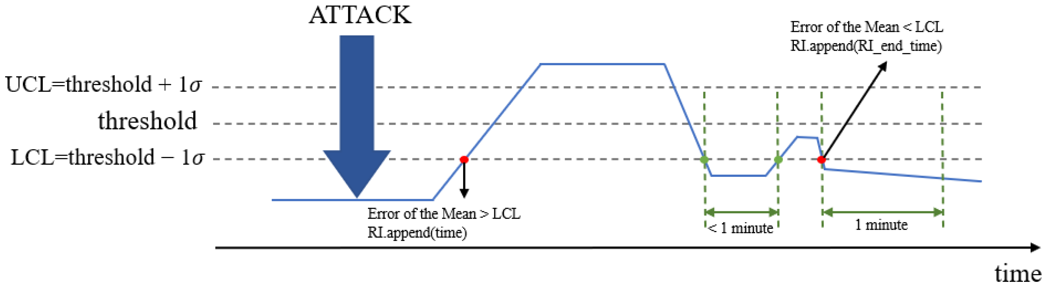
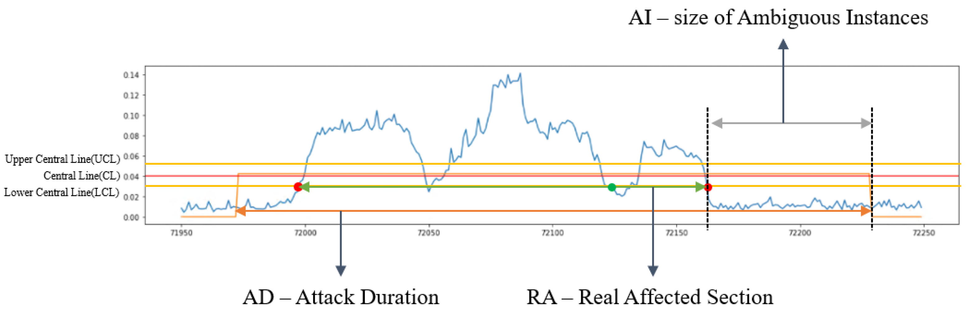
3.2. Defining the Real Affected Section

The starting point of the affected section is where the size of the mean error, which is the blue line in the graph, exceeds the lower limit value. Next, if the magnitude of the average error falls below the lower limit again and lasts for 1 min, the affected section ends. The size of the ambiguous instance is the absolute value of the duration of the attack minus the section affected. Therefore, the start point of the ambiguous instance is obtained by adding 1 to the last point of the attack duration section, and the end point is obtained by adding the start point and the size of the ambiguous instances. Algorithm 1 for finding ambiguous instances are summarized.

Initialize Central Line (CL) to threshold

$$\mathrm{UCL}=\mathrm{CL}+1\sigma$$

$$\mathrm{LCL}=\mathrm{CL}-1\sigma$$

Algorithm 1. Definition of the real affected section

INPUT: CL, UCL, LCL OUTPUT: size of ambiguous instance 1.  attack duration.append(anomalies[i].get_time()[0], anomalies[i].get_time()[1]) 2.  FOR attack duration do 3.    IF error of the mean > LCL then 4.        real affected section.append(current time) 5.    ELSE IF Error of the Mean < LCL then 6.        end time of real affected section = current time 7.        WHILE 1 minute do 8.            IF error of the mean > LCL then 9.               BREAK 10.          ELSE 11.             real affected section.append(end time of real affected section) 12.          ENDIF 13.     ENDWHILE 14.    ENDIF 15.  ENDFOR 16.  IF attack duration[1] > real affected section[1] 17.      size of ambiguous instance = attack duration[1] – real affected section[1] 18.  ELSE 19.      size of ambiguous instance = real affected section[1] - attack duration[1]

During the attack, the algorithm executes the following in Figure 5. First, the magnitude of the mean error and the magnitude of the LCL are compared. If the magnitude of the mean error is larger than that of the LCL, the starting point is appended to the RI, which is the affected section. Next, if the magnitude of the average error is smaller than the LCL, the time point is stored in RI_end_time, which temporarily stores the end time point. Next, if the magnitude of the average error for 1 min is smaller than the LCL, RI_end_time is stored as the end time. However, if the size of the average error becomes larger than the LCL again, the end point must be set again. Because ambiguous instances must be calculated and stored as absolute values, the sizes of AD and RA are compared and stored in AI. The start point is set by adding 1 to the last point of the attack time, and end_id is set by adding AI to start_id.

Figure 5. Example of applying the algorithm to the redefinition of the real affected section.

4. Experimentation

4.1. Model Generation Process

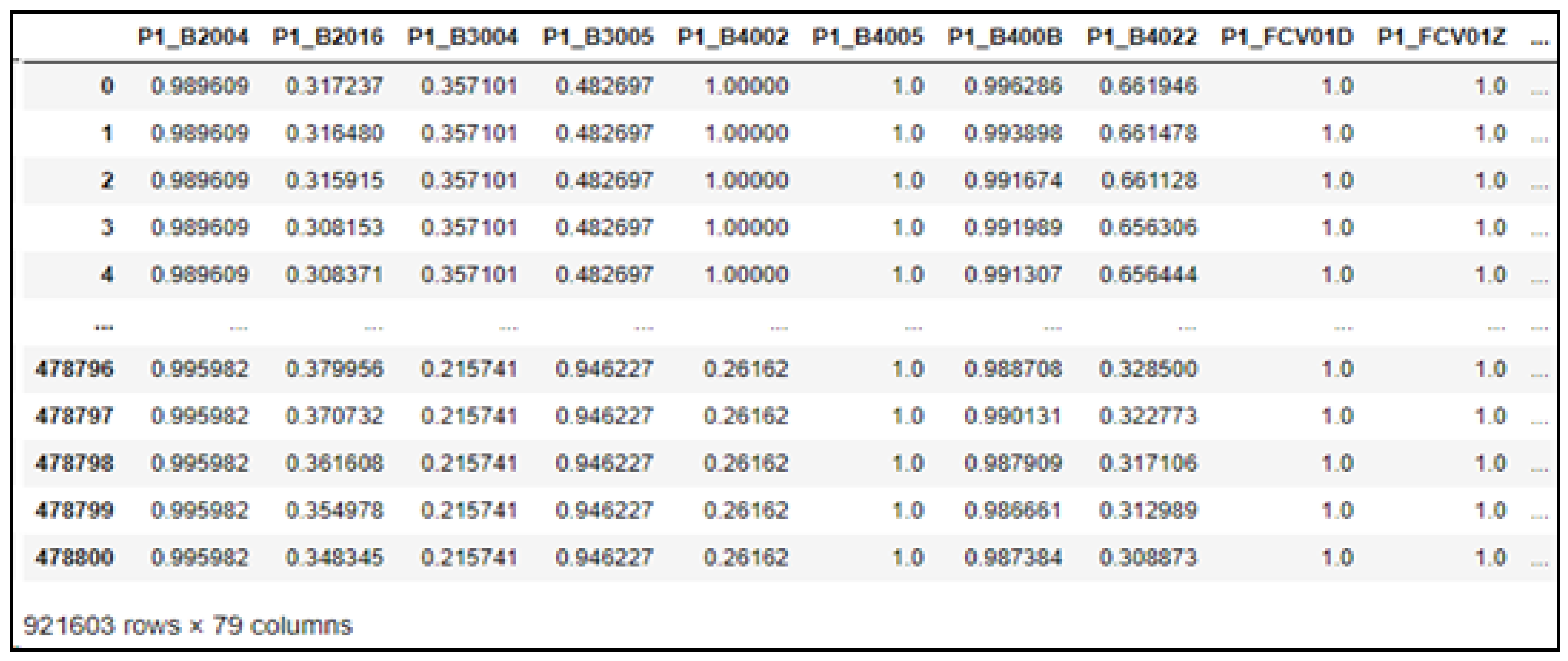
4.1.1. Training Data

This is a learning data selection process for anomaly detection based on industrial control system operation data using artificial intelligence. In the industrial control system operation datasets, SWaT and HAI, the water treatment system operation data collected in Section 2.2 were compared. When comparing data points and attack points between them, SWaT had 60 and 41, and HAI had 78 and 50, respectively. From the diversity of data points and attack points, we determined that HAI had more suitable data for experimentation. The experiment was more suitable for making a case because it had various attack points, while experimenting with SWaT was difficult because there was no labeling for anomalies in recent data.

4.1.2. Choosing a Deep Learning Model

Because the data are time series, selecting a model suitable for time series is necessary. Representative recurrent neural network (RNN), long short-term memory (LSTM), and gated recurrent unit (GRU) algorithms were compared. The RNN [27] receives several input values in chronological order as current inputs and calculates them. However, if the length of the training data is long owing to the structure of the RNN, transferring the previous information to the present is difficult, resulting in a gradient loss problem (long-term dependency). LSTM is an algorithm that solves the gradient loss problem of RNNs. It has a structure in which each unit in the middle layer of a neural network is replaced with a memory unit called an LSTM block. LSTM [28] consists of four gates and one cell state. The gate layer includes a forget gate layer, an input gate layer, the current state, and an output gate layer, and the cell includes the cell state. The cell state indicates the long-term memory. GRU [29] is a simplified version of the cells constituting the LSTM. Compared to LSTM, the structure is simple, and the calculation speed is fast because there are fewer parameters to learn. GRU has two gates: update and reset gates. The update gate determines how much of the previous memory is remembered, and the reset gate decides whether the new input is merged with the old memory.

The performance metric comparison in Table 5 was performed by changing only the model in the HAI 2.0 data and HAI 2.0 baseline code provided by the HAICon2020 Indus-trial Control System Security Threat Detection AI Contest [17]. Table 5 shows the best indicator of the GRU’s performance. Studies have demonstrated that LSTMs show better performances as the amount of data increases. However, without an accurate comparison index, this was directly applied to the data to be tested, and the GRU showing the best performance was selected as the model to be applied to the experiment; PyTorch was used for implementation.

Table 5. Comparison of models based on performance metrics.

Method	Threshold	Performance Metrics
		F1-Score	TaP	TaR
RNN	0.38	78.02	97.20	64.40
LSTM	0.38	81.60	97.40	67.66
GRU	0.38	83.10	97.50	71.50

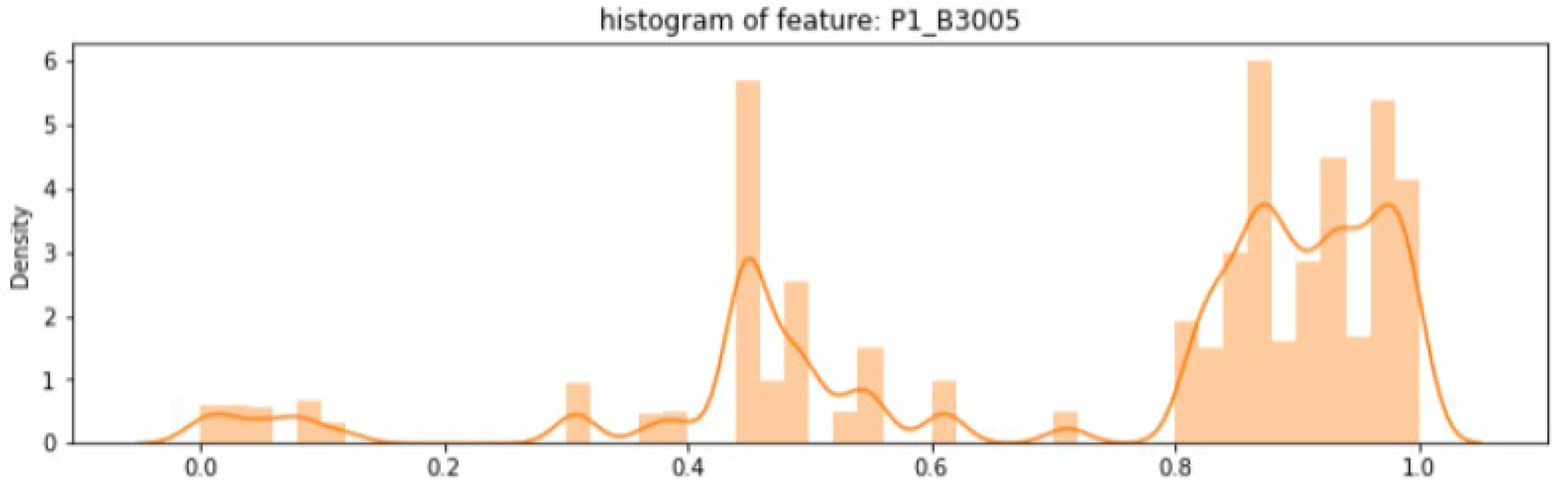
4.1.3. Training Data Preprocessing

The HAI version 21.03 data used as training data consisted of three training data and were provided as a CSV file. Each file is in the form shown in Table 6. Column 1 is the time at which the data were collected, and columns 2 to 80 are the physical values collected from field devices P1, P2, P3, and P4. Column 81 indicates whether an attack event occurred (1) or not (0), and columns 82 to 84 indicate at which stage of the process the attack occurred with attack_P1, attack_P2, and attack_P3, respectively.

Table 6. HAI version 21.03 training data (921,603 rows × 84 columns).

Time	P1_B2004	…	Attack	…	Attack_P3
2020-07-11 12:00:00 AM	0.10121	…	0	…	0
2020-07-11 12:00:01 AM	0.10121	…	0	…	0
…	…	…	…	…	…

The preprocessing of the training data consists of three steps:

• Refining data by removing outliers and missing values;
• Scaling data using normalization;
• Eliminating unnecessary data points with feature graphs.

The first step purifies data by removing outliers and missing values. An outlier is a value with a larger deviation than the normal value it belongs to and is detected using methods such as normal distribution, likelihood, nearest neighbor, density, and clustering. Thereafter, outliers are replaced with the upper or lower limits, the standard deviation of the mean, the absolute mean deviation, and extreme percentiles. The training data of HAI 21.03 are the data collected when operated normally without an attack, all attack labels are 0, and all data points are within the range of the minimum and maximum values. Therefore, there are no outliers. Missing values indicate absent values and are expressed as NA, which must be processed during preprocessing because they cause distortions later when using the model to forecast. Therefore, the missing values are processed by the deletion, substitution, and insertion of the predicted values. The HAI 21.03 training data do not have missing values.

The second step scales the data using normalization, as shown in Figure 6. Data scaling requires preprocessing because if each data range is too wide or small, the data may converge or diverge to 0 during the learning process. For example, P1_B4022 is data that represent temperature with a range from 0 to 40, and P1_FT03 is data that represent pressure with a range from 0 to 2500. Because each range of data differs, either standardization or normalization is used for scaling. Standardization involves distributing data on either side of 0 as a value indicating the distance between the data and the mean. In contrast, normalization in-volves transforming the data range from a minimum of 0 to a maximum of 1 to reduce the effect of the relative size of the data. The minimum and maximum physical data values (columns 2 to 80) were derived from the training data, and normalization was performed.

Figure 6. Normalized training data.

The third step removes unnecessary data points using the feature graph. After normalizing the data points of the training data and converting them to values between 0 and 1, we used the graph to study the characteristics of the data points.

Figure 7 shows the feature graph of data point P1_B3005. Because the values are dis-tributed between 0 and 1 and change over time, they represent the characteristics well. In contrast, the feature graph of data point P1_PCV02D in Figure 8 does not change its value over time. Thus, it is unnecessary data for anomaly detection. Data points with these characteristics were removed. The list of the 22 removed data points includes the following: P1_PCV02D, P1_PP01AD, P1_PP01AR, P1_PP01BD, P1_PP01BR, P1_PP02D, P1_PP02R, P1_STSP, P2_ASD, P2_AutoGO, P2_Emerg, P2_MSD, P2_ManualGO, P2_OnOff, P2_RTR, P2_TripEx, P2_VTR01, P2_VTR02, P2_VTR03, P2_VTR04, P3_LH, and P3_LL.

Figure 7. Feature graph for data point P1_B3005.

Figure 8. Feature graph for data point P1_PCV02D. This feature graph means that the values of the data points do not change over time.

4.1.4. Model Generation

In the model generation process, the model was created considering the following factors:

• Sliding window;
• Number of hidden layers;
• Hidden layer size.

The sliding window [30] is a method of recognizing data according to the characteristics of time series data. The method receives data and remembers the pattern for that window, and it involves input and output values. The input is the value at the beginning of the window, and the output is the value at the end of the window. As a result of the experiment considering the size of the training data for the sliding window input, the size between 75 and 90 was suitable for the experiment. Therefore, it was set at intervals of 5. Table 7 shows the corresponding sliding window input and output values from which the model was created.

Table 7. Sliding window output and input settings.

	Input	Output
1	74	75
2	79	80
3	84	85
4	89	90

The following is the number of hidden layers and their sizes. The stacked GRU used is a multi-layer neural network and consists of input, hidden, and output layers. Each layer comprises nodes, and the number of hidden layers determines how many exist. The model was created using the stacked GRU algorithm selected earlier as the deep learning model. The L1 loss function was used, and AdamW [31] was used as the optimization function. The AdamW function separates the weight decay step of the existing Adam algorithm. During training, the epoch was set to 64, and the model’s parameter with the best loss value was stored. A rectified linear unit (ReLU) was added as an activation function to solve the gradient vanishing problem. In addition, the PyTorch library was used for implementation. Table 8 shows if the learning proceeded according to the size of the sliding window input and output.

Table 8. Comparison of learning models according to the size of the sliding window.

	Input	Output	Wall Time	Loss Value
Case 1	74	75	4 h 50 min 52 s	3.266
Case 2	79	80	5 h 9 min 44 s	3.262
Case 3	84	85	5 h 30 min 13 s	3.301
Case 4	89	90	5 h 50 min 9 s	3.298

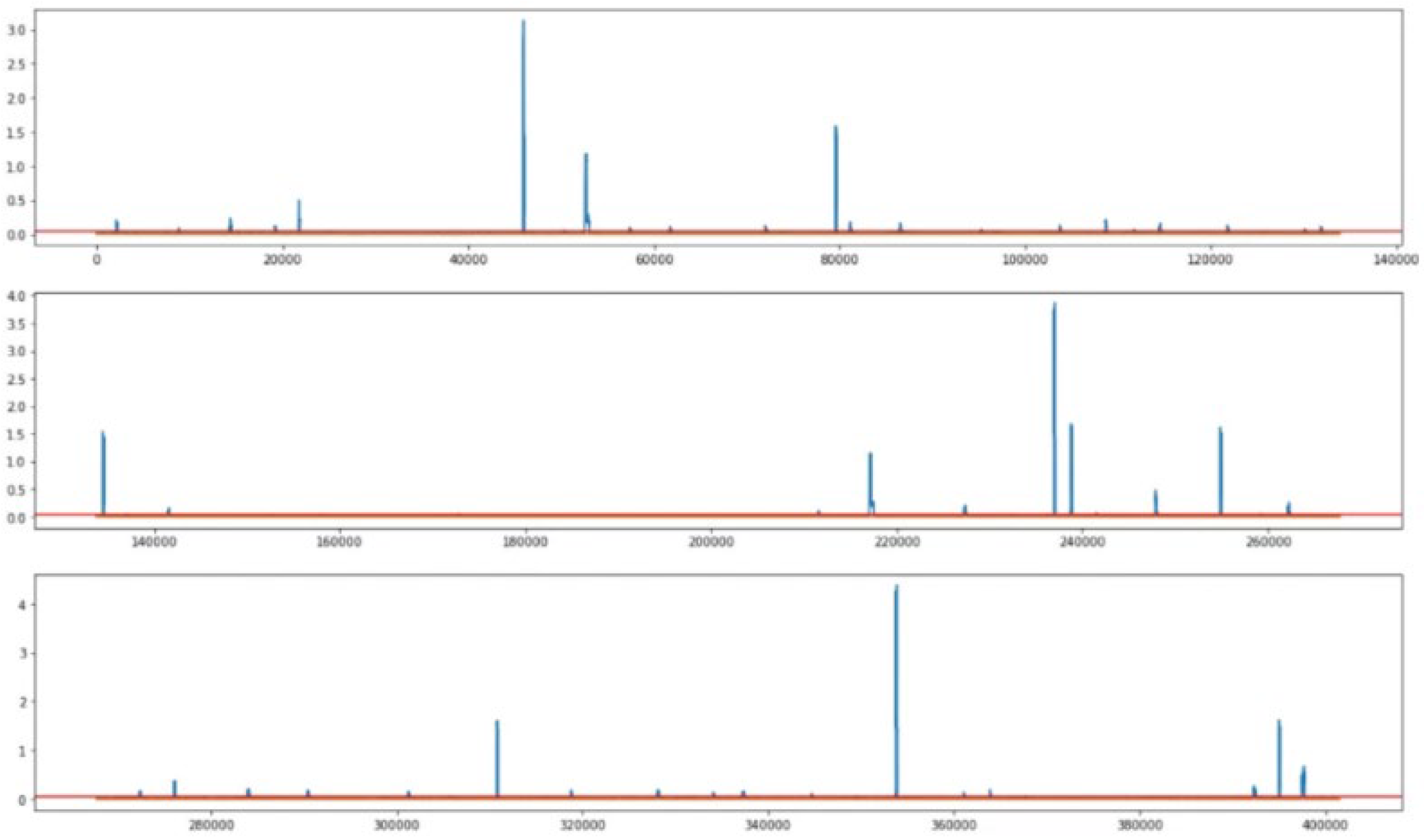
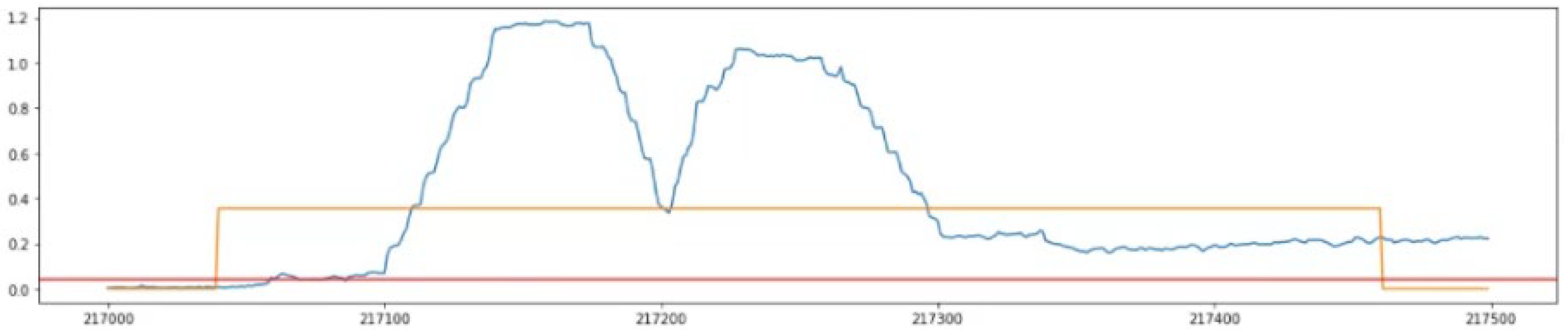
4.2. Anomaly Detection

The test data were formatted as shown in Table 6, and the size was 402,005 rows × 84 columns. In addition, the preprocessing of the test data was performed at the same stage as the training data. The data do not have missing values. The 22 data points were removed, and the data were normalized in the scaling step. This is the process of predicting the results of a test dataset with a model created using a training dataset. In this process, a threshold is used. To determine whether an attack occurs, the average of the calculated differences by the entire field is determined, and then the abnormality is predicted using the threshold value.

The blue line in Figure 9 indicates the size of the average error. If the blue line exceeds the red line, the average error is determined to be abnormal (an attack). Abnormality is indicated by 1, and normality by 0. The predicted label is stored in LABELS, and the correct label of the test set is extracted as ATTACK_LABELS. In this case, the LABELS and ATTACK_LABELS sizes do not match. Because the model learned with the sliding window method, the first part cannot be predicted as much as the sliding window input value. In addition, because the three learning datasets were combined into one set of data, ‘time’ does not continue between the file changes and is thus unpredictable, and the number of predicted labels, LABELS, is less than ATTACK_LABELS. To solve this, we applied a function that fills in the blanks with the normal 0 and remaining values with the judgment of the model.

Figure 9. Average of differences produced by the entire field (blue)/threshold (red). The blue line is the average of the differences calculated by the entire field to determine if there is an attack. The red line is a value arbitrarily specified by the experimenter, and if the blue line exceeds the red line, that point is predicted to be an attack.

As shown in Table 9, the F1-score, TaP, and TaR performance metrics according to the boundary values were derived. The number of detected anomalies was given the highest priority, and subsequently, the highest performance metrics were listed as C1-2, C2-2, C3-1, and C4-2. Among them, C1-2, which had the highest number of detected anomalies and performance metrics, was applied in the analysis of four anomaly detection experiments and evaluation methods. A total of 50 ATTACK_LABELS in the test dataset were labeled, and of these, 36 anomalies were detected as abnormal (attacks) by C1-2: [’1’, ’3’, ’5’, ’6’, ’7’, ’11’, ’12’, ’13’, ’14’, ’16’, ’17’, ’18’, ’22’, ’23’, ’27’, ’28’, ’29’, ’30’, ’31’, ’32’, ’33’, ’34’, ’35’, ’36’, ’37’, ’38’, ’39’, ’40’, ’41’, ’42’, ’43’, ’45’, ’47’, ’48 ’, ’49’, ’50’].

Table 9. Performance metrics according to the threshold of each case.

	Threshold	Number of Anomalies Detected	Performance Metrics
			F1-Score	TaP	TaR
C1-1	0.042	36	0.501	0.413	0.635
C1-2	0.04	36	0.504	0.416	0.639
C1-3	0.38	35	0.503	0.415	0.638
C1-4	0.36	35	0.507	0.417	0.646
C2-1	0.05	36	0.482	0.396	0.611
C2-2	0.047	36	0.496	0.413	0.620
C2-3	0.044	35	0.504	0.425	0.621
C2-4	0.04	34	0.513	0.437	0.622
C3-1	0.047	35	0.484	0.401	0.611
C3-2	0.044	34	0.496	0.417	0.611
C3-3	0.04	33	0.506	0.428	0.619
C3-4	0.038	31	0.487	0.409	0.603
C4-1	0.046	34	0.500	0.417	0.624
C4-2	0.044	34	0.504	0.421	0.628
C4-3	0.042	34	0.501	0.415	0.632
C4-4	0.04	32	0.498	0.420	0.611

4.3. Analysis of Performance Metrics

For the performance evaluation, a section was set in the test dataset. Among the 36 anomalies detected by C1-2, attacks [‘1’, ‘10’, ‘16’, ‘27’, ‘33’] were selected. Those five attacks are shown in Figure 10, Figure 11, Figure 12, Figure 13 and Figure 14.

Figure 10. Section 1: 2000~3000 (Attack 1). The red line is the threshold, and when the blue line crosses the red line, we predict an attack. The orange line is the actual attack range.

Figure 11. Section 2: 71,950~72,250 (Attack 10). The red line is the threshold, and when the blue line crosses the red line, we predict an attack. The orange line is the actual attack range.

Figure 12. Section 3: 114,375~114,675 (Attack 16). The red line is the threshold, and when the blue line crosses the red line, we predict an attack. The orange line is the actual attack range.

Figure 13. Section 4: 217,000~217,500 (Attack 27). The red line is the threshold, and when the blue line crosses the red line, we predict an attack. The orange line is the actual attack range.

Figure 14. Section 5: 262,100~262,500 (Attack 33). The red line is the threshold, and when the blue line crosses the red line, we predict an attack. The orange line is the actual attack range.

Comparison of Performance Metrics by Attack

Table 10 compares the anomaly detection performance of five case intervals selected in the interval setting for performance evaluation. The point-based standard metrics accuracy and F1-score and the range-based standard metrics TaP and TaR were used as performance metrics.

Table 10. Comparison of performance metrics by attack.

Section	Attack	Performance Metrics
		Accuracy	F1-Score	TaP	TaR
1	1	0.953	0.819	0.778	0.865
2	10	0.883	0.654	0.534	0.843
3	16	0.916	0.895	0.895	0.895
4	27	0.952	0.774	0.654	0.940
5	33	0.9875	0.898	0.820	0.992

Five attacks scored an accuracy of 0.88 or higher. If only this metric is checked, we can determine that all attacks were accurately detected. However, referring to the F1-score, which was always lower than the accuracy, as it is a combination of recall and precision, a score between TaP and TaR was derived. When evaluating anomaly detection in time series data by deriving various performance metric results, using point-based performance metrics may lead to an inaccurate evaluation.

As evident in Figure 15, 71,955~72,000 was undetected, 72,000~72,045 was detected, 72,045~72,055 was undetected, 72,055~72,140 was undetected, 72,140~72,160 was detected, and 72,160~72,235 was undetected. From the performance index for this section, the accuracy was 0.883, which is unsuitable as an index for performing anomaly detection. In contrast, the TaP and TaR scores considering the time series were 0.534 and 0.843. For the ambiguous section, the actual duration of the attack was section 71,955~72,235, and it can be inferred that the starting point of the affected section began at 71,980.

Figure 15. Analysis of detected/undetected attacks for Section 2 (Attack 10).

Through this analysis, while an attack was predicted, there is a section in which an attack was detected and a section in which an attack was not detected. Additionally, an attack (red line) occurred, but the blue line does not cross the threshold value, which confirms that the attack is slowly affecting the inside of the system. Therefore, to evaluate the anomaly detection of time series data, time series features must be considered.

Table 11 shows that TaP_d and TaR_d were 1.000 because an attack was detected. TaP_p was derived by considering the ambiguous instance value after calculating the case in which the actual anomaly and prediction overlap. TaR_p was derived by calculating the case in which the anomaly and prediction overlap and then dividing by the number of instances. As such, using TaP and TaR as performance metrics is more suitable for anomaly detection analysis than the accuracy or F1-score.

Table 11. Comparing performance metrics by attack.

TaP = 0.534		TaR = 0.843
TaP_d	TaP_p	TaR_d	TaR_p
1.000	0.365	1.000	0.729

4.4. Application of the Proposed Algorithm

In this section, we define ambiguous intervals by applying the overridden algorithm proposed in Section 3. Figure 16 shows the size of the attack duration section, the section affected, and the ambiguous section of the proposed technique. We set upper and lower lines based on the threshold value, which is the central line. The attack duration section does not need to be calculated as it is a fact defined in the test dataset. Therefore, we need to define the real affected section. Depending on the algorithm, we need to set the start and end points of the real affected section. In the process of setting the end point of the real affected section, the green point is stored in RI_end_time but does not last for 1 min; thus, the subsequent red point is stored in RI_end_time. In addition, because the end point of the attack duration section occurred after the end point of the real affected section, the absolute value of the value obtained by subtracting the end point of the real affected section from the end point of the attack duration section is ambiguous. To derive the TaPR scores using the size of the newly defined ambiguous interval, the interval is substituted into the partial scores for calculating TaR and TaP. Therefore, when calculating S(a’,p), the improved score of TaPR is derived by substituting the size of the newly defined ambiguous section. Derived as performance metrics, these values can be said to have improved the existing performance metrics because the size of the ambiguous section suitable for the attack was defined.

Figure 16. An example of an ambiguous section obtained by applying the proposed algorithm.

5. Conclusions

Cybersecurity threats to industrial control systems that control and manage national infrastructure are on the rise. Therefore, the ability to detect and interpret anomalies in industrial control systems is important. To proactively detect and respond to threats, we need to use a real test-based operating system dataset. Furthermore, it is also important to analyze the results of predicting attacks. Industrial control systems mainly have the characteristics of the time series. However, existing studies used a point-based performance evaluation method that does not consider these time series characteristics. Therefore, we used a real testbed-based operational dataset to perform anomaly detection and derived results using various performance metric methods.

We then redefined the ambiguous section algorithm for TaPR, a range-based performance metric. Traditional TaPR partial scores were calculated at the same rate without considering the characteristics of the attack. It is difficult to conduct an accurate evaluation without considering the characteristics of the attack. Further, it is difficult to pinpoint when attacks on industrial control systems begin and end. Additionally, it is necessary to consider the time when the inside of the system returns to normal even after the attack is over. Therefore, we used the SPC upper and lower limit concepts to reflect the characteristics of these attacks. Using these concepts, we redefined the algorithm of the ambiguous section, and we could derive an evaluation by reflecting the characteristics of the attack. The proposed algorithm allows for more accurate evaluation when performing anomaly detection targeting industrial control system-based time series datasets. However, we need to quantitatively analyze whether the proposed performance indicators are superior to the existing performance metrics. This is because it is difficult to quantitatively express whether the interpretation was accurate, rather than simply determining that the anomaly detection was not successful.

Future research will apply the upper and lower limits applied to the proposed algorithm to anomaly detection. Existing studies only used thresholds to determine anomalies and normality. Each process has its own characteristics after normalizing various process values. Therefore, there is a limit to judging abnormal and normal with only one value. We plan to perform anomaly detection using the upper and lower limits of the SPC applied to the proposed algorithm together with the threshold value.

References

1. Kevin, E.H.; Ronald, E.F. History of Industrial Control System Cyber Incidents, Internet Publication. Available online: https://www.osti.gov/servlets/purl/1505628 (accessed on 8 April 2022).
2. Joseph, S. Evolution of ICS Attacks and the Prospects for Future Disruptive Events, Internet Publication. Available online: https://www.dragos.com/wp-content/uploads/Evolution-of-ICS-Attacks-and-the-Prospects-for-Future-Disruptive-Events-Joseph-Slowik-1.pdf (accessed on 8 April 2022).
3. Stampar, M.; Fertalj, K. Artificial intelligence in network intrusion detection. In Proceedings of the 38th International Convention on Information and Communication Technology, Electronics and Microelectronics, MIPRO, Opatija, Croatia, 25–29 May 2015. [Google Scholar]
4. Hongyu, L.; Bo, L. Machine Learning and Deep Learning Methods for Intrusion Detection Systems: A Survey. Appl. Sci. 2019, 9, 4396. [Google Scholar]
5. Hwang, W.S.; Yun, J.H.; Kim, J.; Kim, H.C. Time-Series Aware Precision and Recall for Anomaly Detection: Considering Variety of Detection Result and Addressing Ambiguous Labeling. In Proceedings of the 28th ACM International Conference on Information and Knowledge Management, CIKM ’19, Beijing, China, 3–7 November 2019; pp. 2241–2244. [Google Scholar]
6. Williams, T.J. The Purdue Enterprise Reference Architecture. IFAC Proc. Vol. 1993, 26 Pt 4, 559–564. [Google Scholar] [CrossRef]
7. CISCO. Network and Security in Industrial Automation Environments—Design Guide; CISCO: San Jose, CA, USA, 2020; pp. 8–13. [Google Scholar]
8. SANS. The Purdue Model and Best Practices for Secure ICS Architectures. Available online: https://www.sans.org/blog/introduction-to-ics-security-part-2/ (accessed on 4 April 2022).
9. Kim, G.H. Industrial Control System Security, 1981th ed.; IITP: Daejeon, Korea, 2021; pp. 5–7. [Google Scholar]
10. Choi, S.O.; Kim, H.C. Energy sector infrastructure security monitoring plan based on MITRE ATT&CK framework. Rev. KIISC 2020, 30, 13–23. [Google Scholar]
11. Han, G.H. Trends in Standards and Testing and Certification Technology-Smart Manufacturing Security Standardization Status. TTA J. 2018, 178, 80–90. [Google Scholar]
12. Korea Industrial Standards. Security for Industrial Automation and Control Systems—Part 4-2: Technical Security Requirements for IACS Components. Available online: https://standard.go.kr/KSCI/standardIntro/getStandardSearchView.do?menuId=919&topMenuId=502&upperMenuId=503&ksNo=KSXIEC62443-4-2&tmprKsNo=KS_C_NEW_2019_3780&reformNo=00 (accessed on 9 February 2022).
13. Shengyi, P.; Thomas, M.; Uttam, A. Developing a Hybrid Intrusion Detection System Using Data Mining for Power Systems. IEEE Trans. Smart Grid 2015, 6, 3104–3113. [Google Scholar]
14. iTrust. BATtle of Attack Detection Algorithms (BATADAL). Available online: https://itrust.sutd.edu.sg/itrust-labs_datasets/dataset_info/ (accessed on 9 February 2022).
15. iTrust. Water Distribution (WADI). Available online: https://itrust.sutd.edu.sg/itrust-labs-home/itrust-labs_wadi/ (accessed on 8 April 2022).
16. iTrust. Secure Water Treatment (SWaT). Available online: https://itrust.sutd.edu.sg/itrust-labs-home/itrust-labs_swat/ (accessed on 8 April 2022).
17. Shin, H.K.; Lee, W.; Yun, J.H.; Min, B.G. Two ICS Security Datasets and Anomaly Detection Contest on the HIL-based Augmented ICS Testbed. In Proceedings of the Cyber Security Experimentation and Test Workshop, CSET ’21, Virtual, CA, USA, 9 August 2021; ACM: New York, NY, USA, 2021; pp. 36–40. [Google Scholar]
18. Shin, H.K.; Lee, W.; Yun, J.H.; Kim, H.C. HAI 1.0: HIL-Based Augmented ICS Security Dataset. In Proceedings of the 13th USENIX Workshop on Cyber Security Experimentation and Test (CSET 20), Boston, MA, USA, 10 August 2020. [Google Scholar]
19. Lee, T.J.; Justin, G.; Nesime, T.; Eric, M.; Stan, Z. Precision and Recall for Range-Based Anomaly Detection. In Proceedings of the SysML Conference, Stanford, CA, USA, 15–16 February 2018. [Google Scholar]
20. Dmitry, S.; Pavel, F.; Andrey, L. Anomaly Detection for Water Treatment System based on Neural Network with Automatic Architecture Optimization. arXiv 2018, arXiv:1807.07282. [Google Scholar]
21. Kim, J.; Yun, J.H.; Kim, H.C. Anomaly Detection for Industrial Control Systems Using Sequence-to-Sequence Neural Networks. arXiv 2019, arXiv:1911.04831. [Google Scholar]
22. Giuseppe, B.; Mauro, C.; Federico, T. Evaluation of Machine Learning Algorithms for Anomaly Detection in Industrial Networks. In Proceedings of the 2019 IEEE International Symposium on Measurements Networking (MN), Catania, Italy, 8–10 July 2019; pp. 1–6. [Google Scholar]
23. Sohrab, M.; Alireza, A.; Kang, K.; Arman, S. A Machine Learning Approach for Anomaly Detection in Industrial Control Systems Based on Measurement Data. Electronics 2021, 10, 407. [Google Scholar]
24. Kim, D.Y.; Hwang, C.W.; Lee, T.J. Stacked-Autoencoder Based Anomaly Detection with Industrial Control System. In Software Engineering, Artificial Intelligence, Networking and Parallel/Distributed Computing; Springer: Cham, Switzerland, 2021; pp. 181–191. [Google Scholar]
25. Roland, C. Statistical process control (SPC). Assem. Autom. 1996, 16, 10–14. [Google Scholar]
26. Vanli, O.A.; Castillo, E.D. Statistical Process Control in Manufacturing; Encyclopedia of Systems and Control; Springer: London, UK, 2014. [Google Scholar]
27. David, E.R.; Geoffrey, E.H.; Ronald, J.W. Learning representations by back-propagating errors. Nature 1986, 323, 533–536. [Google Scholar]
28. Sepp, H.; Jürgen, S. Long Short-Term Memory. Neural Comput. 1997, 8, 1735–1780. [Google Scholar]
29. Cho, K.; Van Merriënboer, B.; Gulcehre, C.; Bahdanau, D.; Bougares, F.; Schwenk, H.; Bengio, Y. Learning phrase representations using RNN encoder-decoder for statistical machine translation. arXiv 2014, arXiv:1406.1078. [Google Scholar]
30. Koç, C.K. Analysis of sliding window techniques for exponentiation. Comput. Math. Appl. 1995, 30, 17–24. [Google Scholar] [CrossRef] [Green Version]
31. Ilya, L.; Frank, H. Decoupled Weight Decay Regularization. In Proceedings of the 7th International Conference on Learning Representations, ICLR, New Orleans, LA, USA, 6–9 May 2019. [Google Scholar]