
A Novel Fusion Pruning Algorithm Based on Information Entropy Stratification and IoT Application


Abstract
:1. Introduction
- Through the network pruning operation, the model size of the network model is smaller, the inference time is less, and the number of operations is smaller.
- Compared to the baseline model (VGG16, ResNet56), the model has better performance.
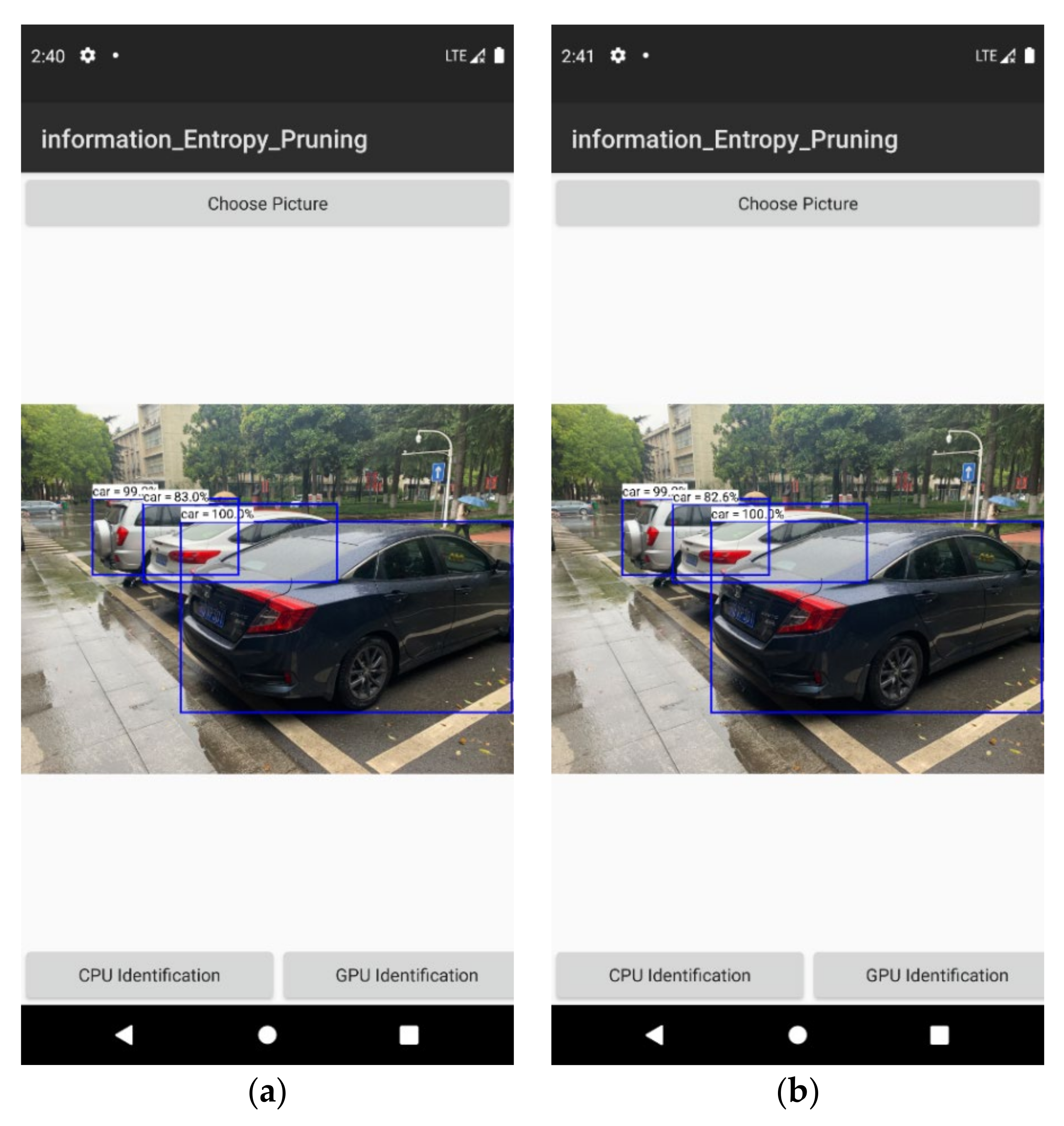
- It maintains a good result for target detection on embedded devices.
2. Related Work
2.1. Unstructured Pruning
2.2. Structured Pruning
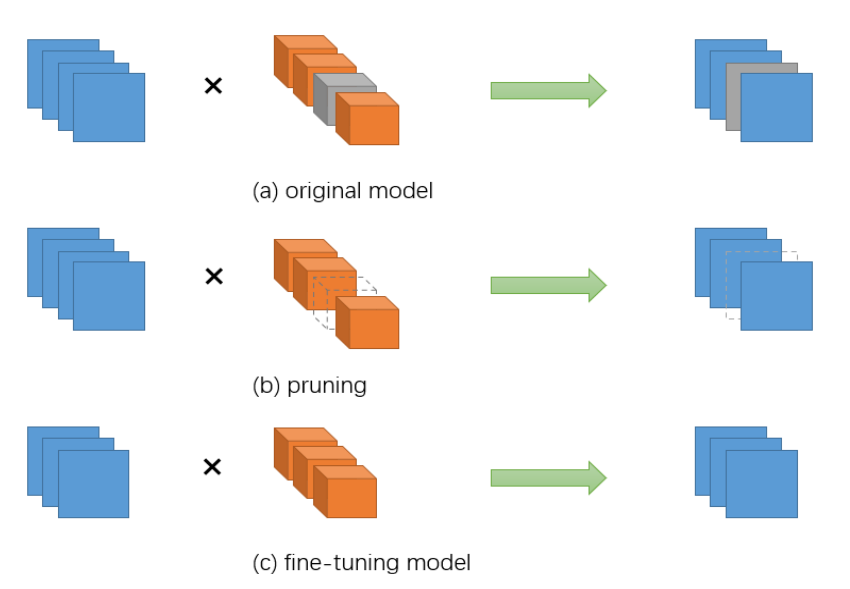
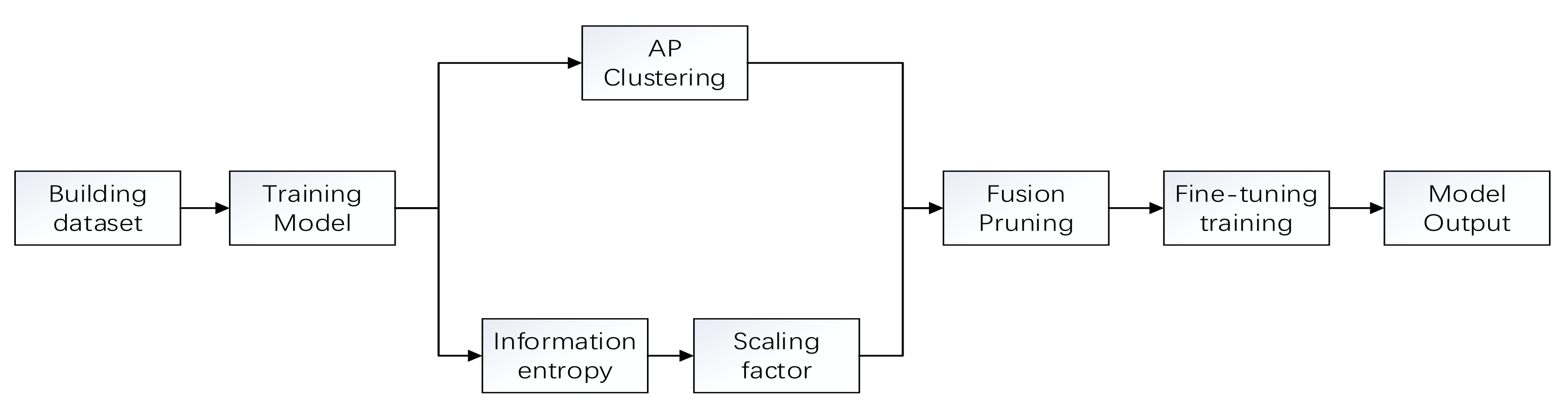
3. Fusion Pruning Algorithm
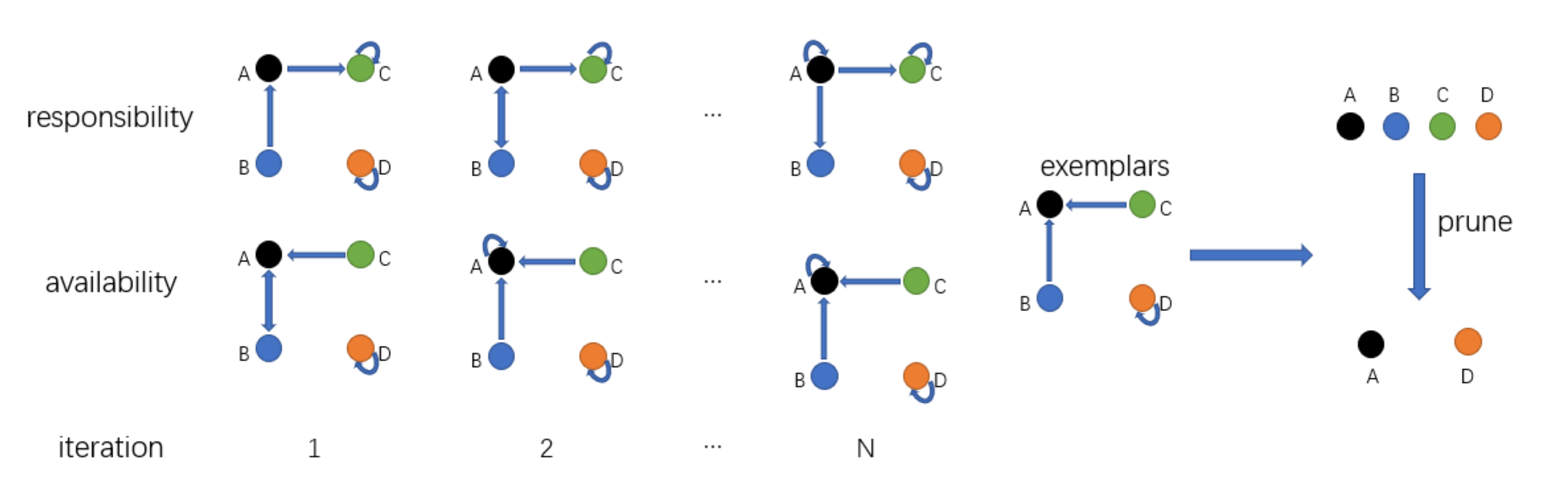
3.1. Filter Pruning Based on Affinity Propagation
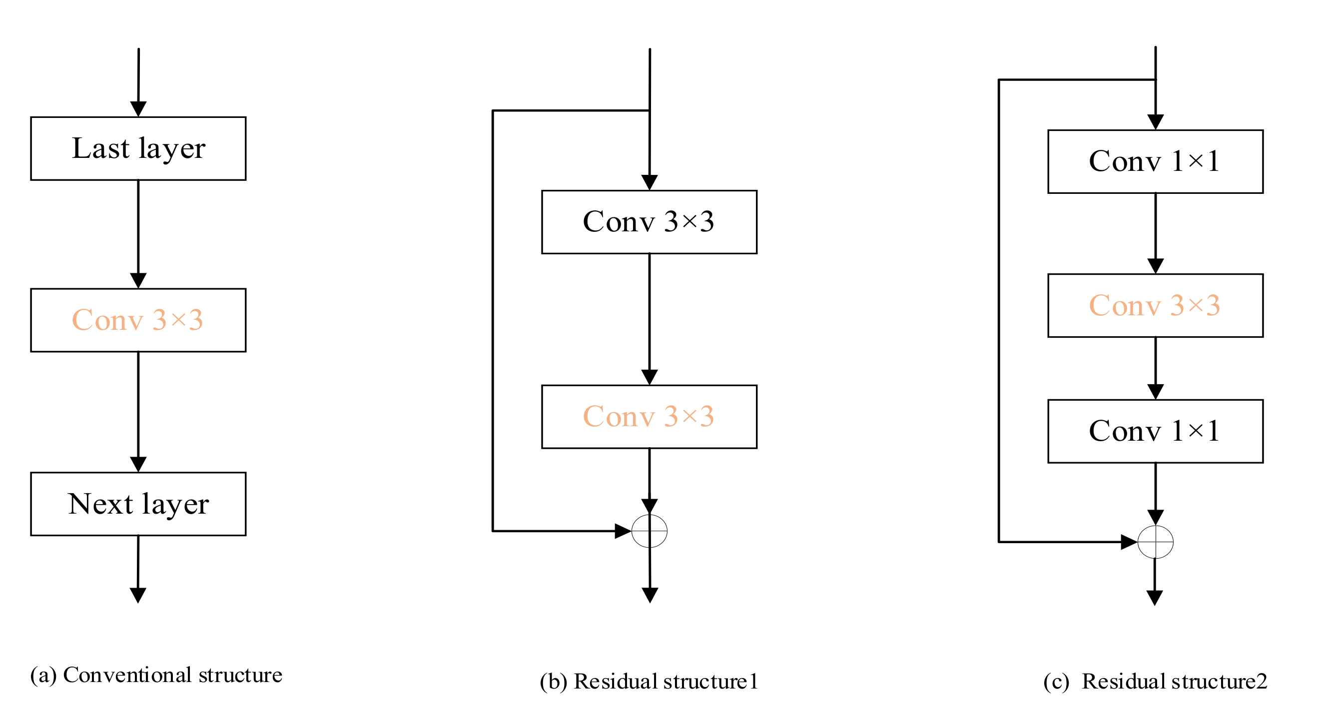
3.2. Channel Pruning Based on Batch Normalization (BN) Layer Scaling Factor
| Algorithm 1 Batch Normalizing Transform. |
| Input: values of x over a mini-batch: B = {}; Parameters to be learned: |
| Output. |
| //mini-batch mean |
| 2. //mini-batch variance |
| 3. //normalize |
| 4. //scale and shift |
3.3. Fusion Pruning
| Algorithm 2 The K-Means Clustering. | |
| Input: sample set | |
| Number of clusters K | |
| Process: | |
| 1: | K samples are randomly selected from T as the initial mean vector: |
| 2: | repeat |
| 3: | Cause |
| 4: | for do |
| 5: | Calculate the distance between the sample and each mean vector : ; |
| 6: | Determined from the nearest mean vector of the cluster markers: ; |
| 7: | Place the samples Classify into the appropriate clusters |
| 8: | end for |
| 9: | for do |
| 10: | Calculate the new mean vector: ; |
| 11: | if then |
| 12: | Update the current mean vector to ; |
| 13: | else |
| 14: | Keep the current mean vector constant |
| 15: | end if |
| 16: | end for |
| 17: | until none of the current mean vectors are updated |
| Output: Cluster division | |
| Algorithm 3 Fusion Pruning Algorithm. |
| 1: Trained the original VGG16 network on the training set. |
| 2: Selection of convolutional layers for prunable networks. |
| 3: Clustering of the network to obtain m categories. |
| 4: Obtain the redundant filters to be removed, based on the samples from each category. |
| 5: After step 2, calculate the entropy value using a range of scaling factor values. 6: Determine the pruning rate of each layer by dividing into N classes using k-means. 7: Ranking the scaling factors of each convolutional layer and obtaining the channels to be removed according to the pruning rate P of that layer. |
| 8: Merge the results obtained in steps four and seven. |
| 9: Remove the sum obtained in step eight after step two to obtain the streamlined network structure. |
| 10: Fine-tuning the new network on the training data to get the final model. |
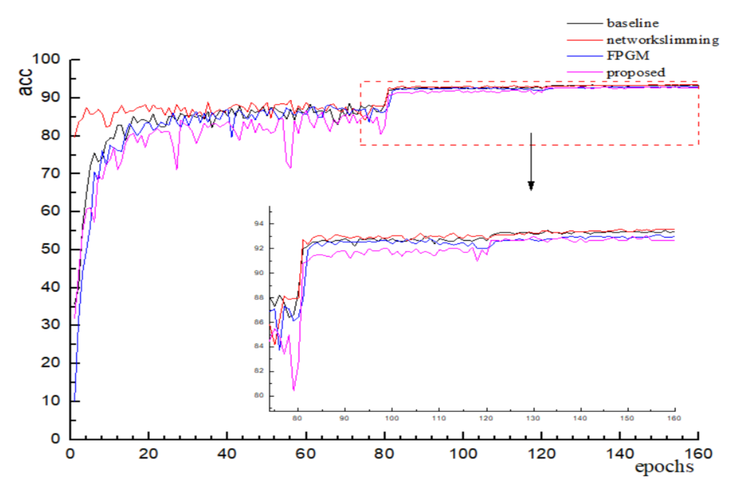
4. Experiment
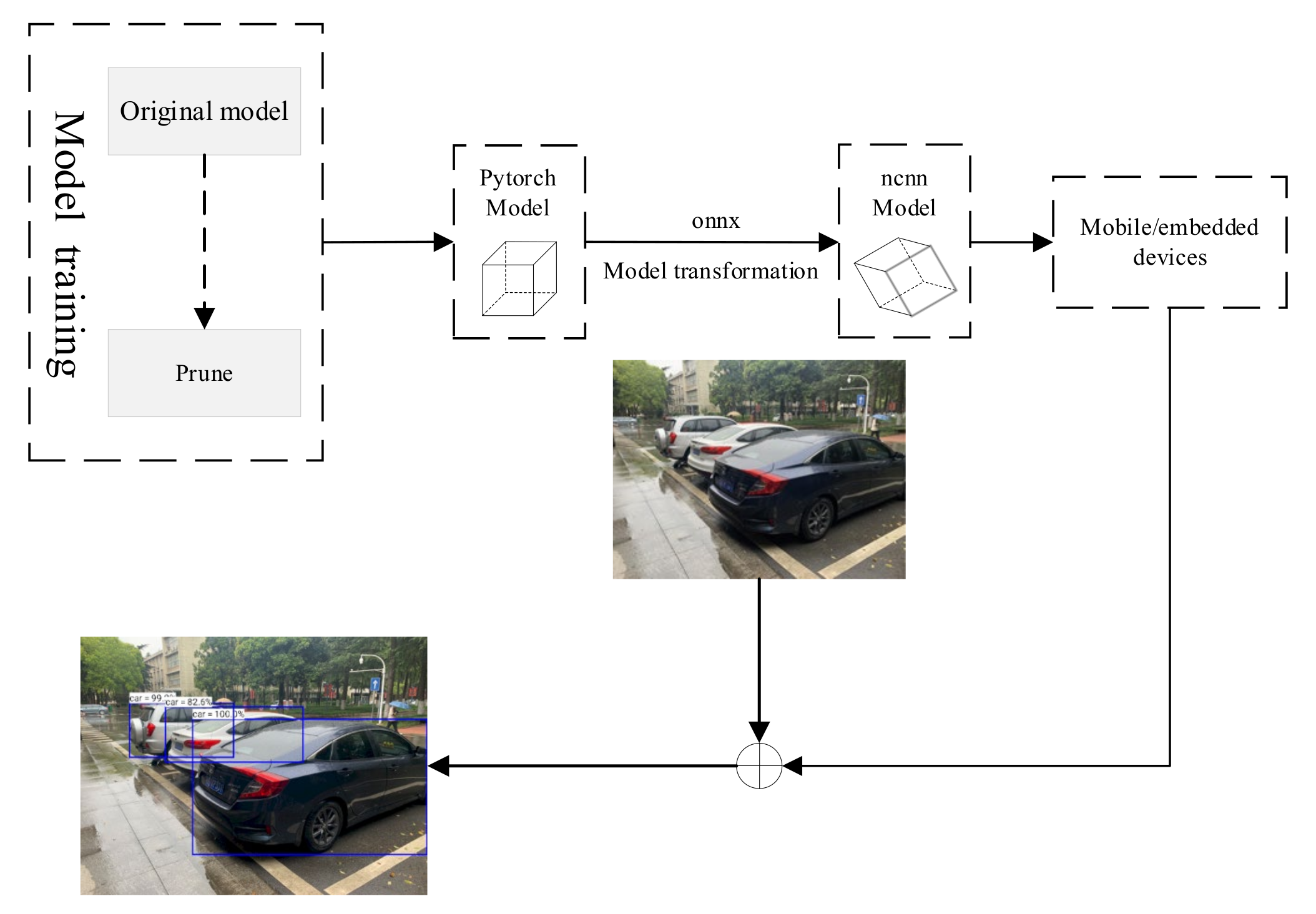
5. Case Study
5.1. Development of the Internet of Things (IoT)
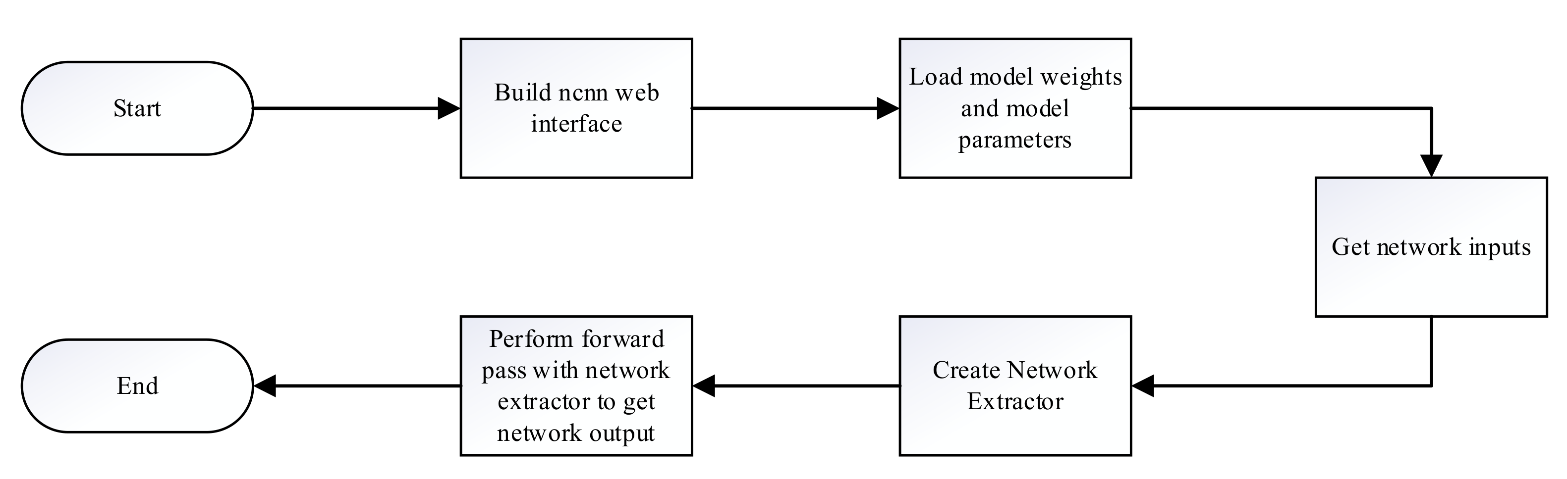
5.2. NCNN Framework
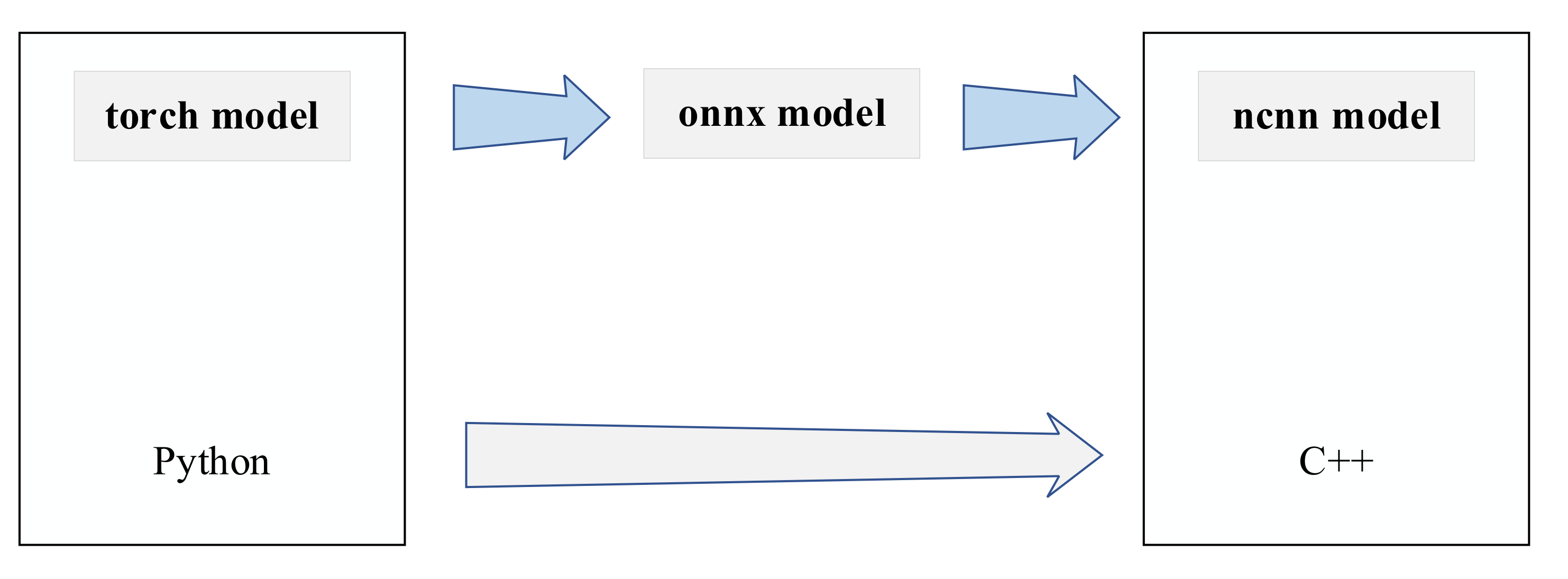
5.3. Model Conversion
5.4. System Construction
6. Conclusions
Author Contributions
Funding
Conflicts of Interest
References
- Simonyan, K.; Zisserman, A. Very deep convolutional networks for large-scale lmage recognition. arXiv 2014, arXiv:1409.1556. [Google Scholar]
- Szegedy, C.; Liu, W.; Jia, Y.; Sermanet, P.; Rabinovich, A. Going Deeper with Convolutions. In Proceedings of the IEEE Conference on Computer Vision and Pattern Recognition, Boston, MA, USA, 7–12 June 2015. [Google Scholar] [CrossRef] [Green Version]
- He, K.; Zhang, X.; Ren, S.; Sun, J. Deep Residual Learning for Image Recognition. In Proceedings of the 2016 IEEE Conference on Computer Vision and Pattern Recognition (CVPR), Las Vegas, NV, USA, 27–30 June 2016. [Google Scholar]
- Huang, G.; Liu, Z.; Laurens, V.; Weinberger, K.Q. Densely Connected Convolutional Networks. In Proceedings of the IEEE Conference on Computer Vision and Pattern Recognition, Honolulu, HI, USA, 21–26 July 2017. [Google Scholar]
- Iandola, F.N.; Han, S.; Moskewicz, M.W.; Ashraf, K.; Dally, W.J.; Keutzer, K. SqueezeNet: AlexNet-level accuracy with 50× fewer parameters and <0.5 MB model size. arXiv 2016, arXiv:1602.07360. [Google Scholar]
- Howard, A.G.; Zhu, M.; Chen, B.; Kalenichenko, D.; Wang, W.; Weyand, T.; Andreetto, M.; Adam, H. MobileNets: Efficient Convolutional Neural Networks for Mobile Vision Applications. arXiv 2017, arXiv:1704.04861. [Google Scholar]
- Zhang, X.; Zhou, X.; Lin, M.; Sun, J. ShuffleNet: An Extremely Efficient Convolutional Neural Network for Mobile Devices. arXiv 2017, arXiv:1707.01083v2. [Google Scholar]
- He, Y.; Liu, P.; Wang, Z.; Hu, Z.; Yang, Y. Filter Pruning via Geometric Median for Deep Convolutional Neural Networks Acceleration. In Proceedings of the 2019 IEEE/CVF Conference on Computer Vision and Pattern Recognition (CVPR), Long Beach, CA, USA, 16–20 June 2019. [Google Scholar]
- Li, H.; Kadav, A.; Durdanovic, I.; Samet, H.; Graf, H.P. Pruning Filters for Efficient ConvNets. arXiv 2016, arXiv:1608.08710. [Google Scholar]
- Zhang, X.; He, Y.; Jian, S. Channel Pruning for Accelerating Very Deep Neural Networks. In Proceedings of the IEEE International Conference on Computer Vision, Venice, Italy, 22–29 October 2017. [Google Scholar]
- Zhao, M.; Li, M.; Peng, S.-L.; Li, J. A Novel Deep Learning Model Compression Algorithm. Electronics 2022, 11, 1066. [Google Scholar] [CrossRef]
- Lin, M.; Ji, R.; Wang, Y.; Zhang, Y.; Zhang, B.; Tian, Y.; Shao, L. HRank: Filter Pruning using High-Rank Feature Map. In Proceedings of the IEEE/CVF Conference on Computer Vision and Pattern Recognition, Seattle, WA, USA, 14–19 June 2020. [Google Scholar]
- Wang, W.; Fu, C.; Guo, J.; Cai, D.; He, X. COP: Customized Deep Model Compression via Regularized Correlation-Based Filter-Level Pruning. arXiv 2019, arXiv:1906.10337. [Google Scholar]
- Ghimire, D.; Kil, D.; Kim, S.-H. A Survey on Efficient Convolutional Neural Networks and Hardware Acceleration. Electronics 2022, 11, 945. [Google Scholar] [CrossRef]
- Chin, T.W.; Ding, R.; Zhang, C.; Marculescu, D. Towards Efficient Model Compression via Learned Global Ranking. arXiv 2019, arXiv:1904.12368. [Google Scholar]
- De Campos Souza, P.V.; Bambirra Torres, L.C.; Lacerda Silva, G.R.; Braga, A.d.P.; Lughofer, E. An Advanced Pruning Method in the Architecture of Extreme Learning Machines Using L1-Regularization and Bootstrapping. Electronics 2020, 9, 811. [Google Scholar] [CrossRef]
- Lecun, Y. Optimal Brain Damage. Neural Inf. Proc. Syst. 1990, 2, 598–605. [Google Scholar]
- Hassibi, B.; Stork, D.G. Second order derivatives for network pruning: Optimal brain surgeon. In Proceedings of the Advances in Neural Information Processing Systems, Denver, CO, USA, 30 November–3 December 1992. [Google Scholar]
- Dong, X.; Chen, S.; Pan, S.J. Learning to Prune Deep Neural Networks via Layer-wise Optimal Brain Surgeon. In Proceedings of the Advances in Neural Information Processing Systems, Long Beach, CA, USA, 4–9 December 2017. [Google Scholar]
- Han, S.; Pool, J.; Tran, J.; Dally, W.J. Learning both Weights and Connections for Efficient Neural Networks; MIT Press: Cambridge, MA, USA, 2015. [Google Scholar]
- Guo, Y.; Yao, A.; Chen, Y. Dynamic Network Surgery for Efficient DNNs. In Proceedings of the Nips, Barcelona, Spain, 5–10 December 2016. [Google Scholar]
- Zhou, A.Z.; Luo, K. Sparse Dropout Regularization Method for Convolutional Neural Networks. J. Chin. Comput. Syst. 2018, 39, 1674–1679. [Google Scholar]
- Srinivas, S.; Babu, R.V. Data-free parameter pruning for Deep Neural Networks. In Proceedings of the Computer Science, Swansea, UK, 7–10 September 2015; pp. 2830–2838. [Google Scholar]
- Chen, W.; Wilson, J.T.; Tyree, S.; Weinberger, K.Q.; Chen, Y. Compressing Neural Networks with the Hashing Trick. In Proceedings of the Computer Science, Swansea, UK, 7–10 September 2015; pp. 2285–2294. [Google Scholar]
- Zhuang, L.; Li, J.; Shen, Z.; Gao, H.; Zhang, C. Learning Efficient Convolutional Networks through Network Slimming. In Proceedings of the 2017 IEEE International Conference on Computer Vision (ICCV), Venice, Italy, 22–29 October 2017. [Google Scholar]
- Kang, M.; Han, B. Operation-Aware Soft Channel Pruning using Differentiable Masks. In Proceedings of the International Conference on Machine Learning, Shanghai, China, 6–8 November 2020. [Google Scholar]
- Yan, Y.; Li, C.; Guo, R.; Yang, K.; Xu, Y. Channel Pruning via Multi-Criteria based on Weight Dependency. In Proceedings of the 2021 International Joint Conference on Neural Networks, Shenzhen, China, 18–22 July 2020. [Google Scholar]
- He, Y.; Kang, G.; Dong, X.; Fu, Y.; Yang, Y. Soft Filter Pruning for Accelerating Deep Convolutional Neural Networks. arXiv 2018, arXiv:1808.06866. [Google Scholar]
- Luo, J.H.; Wu, J.; Lin, W. ThiNet: A Filter Level Pruning Method for Deep Neural Network Compression. In Proceedings of the 2017 IEEE International Conference on Computer Vision (ICCV), Venice, Italy, 22–29 October 2017. [Google Scholar]
- Yang, W.; Jin, L.; Wang, S.; Cu, Z.; Chen, X.; Chen, L. Thinning of Convolutional Neural Network with Mixed Pruning. IET Image Processing 2019, 13, 779–784. [Google Scholar] [CrossRef]
- Hu, H.; Peng, R.; Tai, Y.W.; Tang, C.K. Network Trimming: A Data-Driven Neuron Pruning Approach towards Efficient Deep Architectures. arXiv 2016, arXiv:1607.03250. [Google Scholar]
- Molchanov, P.; Tyree, S.; Karras, T.; Aila, T.; Kautz, J. Pruning Convolutional Neural Networks for Resource Efficient Transfer Learning. arXiv 2016, arXiv:1611.06440. [Google Scholar]
- Luo, J.H.; Wu, J. An Entropy-based Pruning Method for CNN Compression. arXiv 2017, arXiv:1706.05791. [Google Scholar]
- Yu, R.; Li, A.; Chen, C.F.; Lai, J.H.; Davis, L.S. NISP: Pruning Networks Using Neuron Importance Score Propagation. In Proceedings of the IEEE/CVF Conference on Computer Vision & Pattern Recognition, Salt Lake City, UT, USA, 18–22 June 2018. [Google Scholar]
- Lin, M.; Ji, R.; Chen, B.; Chao, F.; Liu, J.; Zeng, W.; Tian, Y.; Tian, Q. Training Compact CNNs for Image Classification using Dynamic-coded Filter Fusion. arXiv 2021, arXiv:2107.06916. [Google Scholar]
- Wen, W.; Wu, C.; Wang, Y.; Chen, Y.; Li, H. Learning Structured Sparsity in Deep Neural Networks. In Proceedings of the Advances in Neural Information Processing Systems, Barcelona, Spain, 5–10 December 2016. [Google Scholar]
- Huang, Z.; Wang, N. Data-Driven Sparse Structure Selection for Deep Neural Networks. In Proceedings of the European Conference on Computer Vision (ECCV), Venice, Italy, 22–29 October 2017. [Google Scholar]
- Lin, M.; Ji, R.; Li, S.; Wang, Y.; Ye, Q. Network Pruning Using Adaptive Exemplar Filters. IEEE Trans. Neural Netw. Learn. Syst. 2021. [Google Scholar] [CrossRef]
- Lin, M.; Ji, R.; Li, S.; Ye, Q.; Tian, Y.; Liu, J.; Tian, Q. Filter Sketch for Network Pruning. arXiv 2020, arXiv:2001.08514. [Google Scholar] [CrossRef]
- Li, Y.; Lin, S.; Zhang, B.; Liu, J.; Ji, R. Exploiting Kernel Sparsity and Entropy for Interpretable CNN Compression. In Proceedings of the 2019 IEEE/CVF Conference on Computer Vision and Pattern Recognition (CVPR), Long Beach, CA, USA, 15–20 June 2019. [Google Scholar]
- Kumar, T.A.; Rajmohan, R.; Pavithra, M.; Ajagbe, S.A.; Hodhod, R.; Gaber, T. Automatic Face Mask Detection System in Public Transportation in Smart Cities Using IoT and Deep Learning. Electronics 2022, 11, 904. [Google Scholar] [CrossRef]
- Tarek, H.; Aly, H.; Eisa, S.; Abul-Soud, M. Optimized Deep Learning Algorithms for Tomato Leaf Disease Detection with Hardware Deployment. Electronics 2022, 11, 140. [Google Scholar] [CrossRef]


| Acc | Flops (M) | Pruning Rate (%) | Param (M) | Pruning Rate (%) | ||
|---|---|---|---|---|---|---|
| VGGNet-16 | baseline | 0.9351 | 626.39 | - | 14.72 | - |
| NS [25] | 0.9355 | 306.68 | 51.04 | 1.83 | 87.6 | |
| FPGM | 0.9357 | 412.06 | 34.22 | 5.25 | 64.33 | |
| proposed | 0.9312 | 153.21 | 75.54 | 1.37 | 90.69 | |
| ResNet-56 | baseline | 0.9323 | 126.52 | - | 0.85 | - |
| NS [25] | 0.9291 | 64.92 | 48.69 | 0.41 | 51.76 | |
| DCFF [35] | 0.9326 | 55.78 | 55.91 | 0.36 | 57.65 | |
| FilterSketch [39] | 0.9316 | 73.36 | 42.02 | 0.51 | 40 | |
| HRank [12] | 0.9319 | 62.70 | 50.44 | 0.49 | 42.35 | |
| KSE(G = 4) [40] | 0.9322 | 60.03 | 52.55 | 0.43 | 49.41 | |
| proposed | 0.9321 | 45.78 | 63.82 | 0.31 | 63.53 |
| Model | Time |
|---|---|
| original model | 573.04 ms |
| proposed model | 252.84 ms |
Publisher’s Note: MDPI stays neutral with regard to jurisdictional claims in published maps and institutional affiliations. |
© 2022 by the authors. Licensee MDPI, Basel, Switzerland. This article is an open access article distributed under the terms and conditions of the Creative Commons Attribution (CC BY) license (https://creativecommons.org/licenses/by/4.0/).
Share and Cite
Zhao, M.; Hu, M.; Li, M.; Peng, S.-L.; Tan, J. A Novel Fusion Pruning Algorithm Based on Information Entropy Stratification and IoT Application. Electronics 2022, 11, 1212. https://doi.org/10.3390/electronics11081212
Zhao M, Hu M, Li M, Peng S-L, Tan J. A Novel Fusion Pruning Algorithm Based on Information Entropy Stratification and IoT Application. Electronics. 2022; 11(8):1212. https://doi.org/10.3390/electronics11081212
Chicago/Turabian StyleZhao, Ming, Min Hu, Meng Li, Sheng-Lung Peng, and Junbo Tan. 2022. "A Novel Fusion Pruning Algorithm Based on Information Entropy Stratification and IoT Application" Electronics 11, no. 8: 1212. https://doi.org/10.3390/electronics11081212
APA StyleZhao, M., Hu, M., Li, M., Peng, S.-L., & Tan, J. (2022). A Novel Fusion Pruning Algorithm Based on Information Entropy Stratification and IoT Application. Electronics, 11(8), 1212. https://doi.org/10.3390/electronics11081212