Hybrid Architecture Based on CNN and Transformer for Strip Steel Surface Defect Classification

Abstract

Strip steel surface defects occur frequently during the manufacturing process, and these defects cause hidden risks in the use of subsequent strip products. Therefore, it is crucial to classify the strip steel’s surface defects accurately and efficiently. Most classification models of strip steel surface defects are generally based on convolutional neural networks (CNNs). However, CNNs, with local receptive fields, do not have admirable global representation ability, resulting in poor classification performance. To this end, we proposed a hybrid network architecture (CNN-T), which merges CNN and Transformer encoder. The CNN-T network has both strong inductive biases (e.g., translation invariance, locality) and global modeling capability. Specifically, CNN first extracts low-level and local features from the images. The Transformer encoder then globally models these features, extracting abstract and high-level semantic information and finally sending them to the multilayer perceptron classifier for classification. Extensive experiments show that the classification performance of CNN-T outperforms pure Transformer networks and CNNs (e.g., GoogLeNet, MobileNet v2, ResNet18) on the NEU-CLS dataset (training ratio is 80%) with a 0.28–2.23% improvement in classification accuracy, with fewer parameters (0.45 M) and floating-point operations (0.12 G).

1. Introduction

As global manufacturing changes, the standards for strip quality are also increasing. Hot-rolled strip steel is a multi-functional low carbon steel with excellent properties such as low hardness, easy processing, and excellent malleability. It has been widely used in automobile manufacturing [1], bridges [2], and pipelines. However, a hot-rolled strip steel surface commonly causes defects (e.g., rolled-in scale, cracks, pitted surface) in the production process due to numerous factors such as production environment, materials, rolling equipment, and processing technology [3]. The performance of the strip steel (e.g., corrosion resistance, wear resistance, and toughness) may change due to these defects, which will reduce the quality of the final product [4]. Therefore, it is crucial to classify the strip steel’s surface defects accurately and efficiently.

A convolutional neural network (CNN) is preferable to other types (e.g., artificial neural network, recurrent neural network) of deep learning models. Specifically, CNN learns local patterns and captures promising semantic information, and it is also known to be efficient (e.g., GPU parallelization, less number of parameters) compared to other types [5,6]. The traditional CNNs and their variants, such as ResNet [7], SENet [8], ShuffleNet [9], and MobileNet [10], are commonly used to classify strip steel surface defects. However, CNN has an aptitude for local features but not global features since each convolutional operation only correlates pixels within a local area. Thus, there are certain limitations and challenges when considering CNN as a feature extractor to extract the features of the strip steel’s surface defects images [11]. In contrast, Transformer [12] networks based on self-attention mechanisms ignore local information in the early stages, but they have outstanding abilities in global modeling [13]. To this end, we propose a hybrid architecture based on CNN and Transformer (CNN-T), which has both satisfactory inductive bias and global modeling capabilities.

The main contributions to this paper are listed below.

(1) We propose a hybrid network architecture (CNN-T) based on CNN and Transformer with prior knowledge and global modeling ability, outperforming pure transformers and most CNNs (e.g., GoogLeNet, MobileNet v2, ResNet18) on the NEU-CLS dataset.

(2) The data samples in the experiments are insufficient, which cause severe overfitting in training. We explore several data augmentation strategies to address this problem, such as cropping, Gaussian noise, pseudo-color augmentation, etc., which increase the number and diversity of samples.

The rest of this paper is as follows. Section 2 introduces the related work. Section 3 details the CNN, the Visual Transformer (ViT) [14], and the proposed architecture CNN-T. Section 4 describes the data processing work. Section 5 shows the experiment’s details and analyzes the experimental results. Section 7 gives the conclusion of this paper.

2. Related Works

In the past, professionals identified defects in a non-automated way, which were inefficient and error-prone [15,16,17]. In addition, different experienced professionals will make diverse judgments for the same defects, resulting in incorrect types and grades of strip steel defects, thus reducing the reliability of defect identification. In general, the recognition results obtained by relying on the subjective estimation of professionals are unreliable [18].

To overcome the shortcomings of manual identification, scholars have studied various algorithms based on machine learning technology. Ref. [19] proposed a classification method combining the Grayscale Covariance Matrix (GLCM) and the Discrete Shear Transform (DST). First, multi-directional shear features are extracted from the images, followed by a GLCM calculation. Then it performs main components analysis with high-dimensional feature vectors, and finally, it is sent to the support vector machine (SVM) to identify the surface defects of the strip steel. Ref. [20] proposed a novel multi-hypersphere SVM with additional information (MHSVM+) method, which learns extra information hidden in defect data sets through an additive learning paradigm. It has better classification accuracy on defect datasets, specifically damaged datasets. Ref. [21] proposed a one-class classification method based on generative adversarial network (GAN) [22] and SVM for the identification of strip steel’s surface defect. It uses GAN generated features to train an SVM classifier. In addition, it improves the loss function to enhance the stability of the model. However, the above conventional Machine Learning algorithms usually require complex feature engineering, which adds significantly to the cost.

In recent years, deep learning-based methods have achieved remarkable success for image classification tasks, especially CNN. CNN has powerful characterization capabilities and has shown excellent performance in strip surface defect recognition [23,24,25]. Ref. [23] adopted GoogLeNet [26] as the base model and added an identity mapping to it, which improved it to some extent. In addition, data augmentation strategies augmented the dataset to alleviate overfitting. Ref. [24] proposed an end-to-end and efficient model based on SqueezeNet [8]. SqueezeNet added the multiple receptive fields module, which can generate scale-related high-level features. It is suitable for low-level feature training and enables fast yet robust classification for strip steel surface defects. Ref. [25] proposed an intelligent recognition system of surface defects for hot-rolled steel strip images using modified AlexNet [27] and SVM. Classification models based on CNN have great fitting ability but do not have excellent global representation ability due to the limitation of receptive fields.

In addition to using pure CNNs for classification tasks, some researchers have also explored combining CNNs and Transformers with the ability to capture long-range dependencies, aiming to fully integrate the advantages of both CNNs and Transformers to improve classification performance. Ref. [28] combined CNN with the Bidirectional Encoder Representations from Transformers (BERT) [29] for Intent Determination. First, context representations of a sentence are obtained through BERT, and then these representations are fed into CNN to get feature maps. Finally, the predicted labels are given by the softmax layer. Ref. [30] introduced two convolution-based operations into the ViT to improve the performance and efficiency of ViT on the ImageNet dataset.

In contrast to the above works, this work aims to create a hybrid architecture based on CNN and a Transformer encoder (CNN-T), which employs a Transformer encoder with global modeling capability to overcome the limitation of pure CNN, which can only capture local information.

3. Methods

3.1. CNN

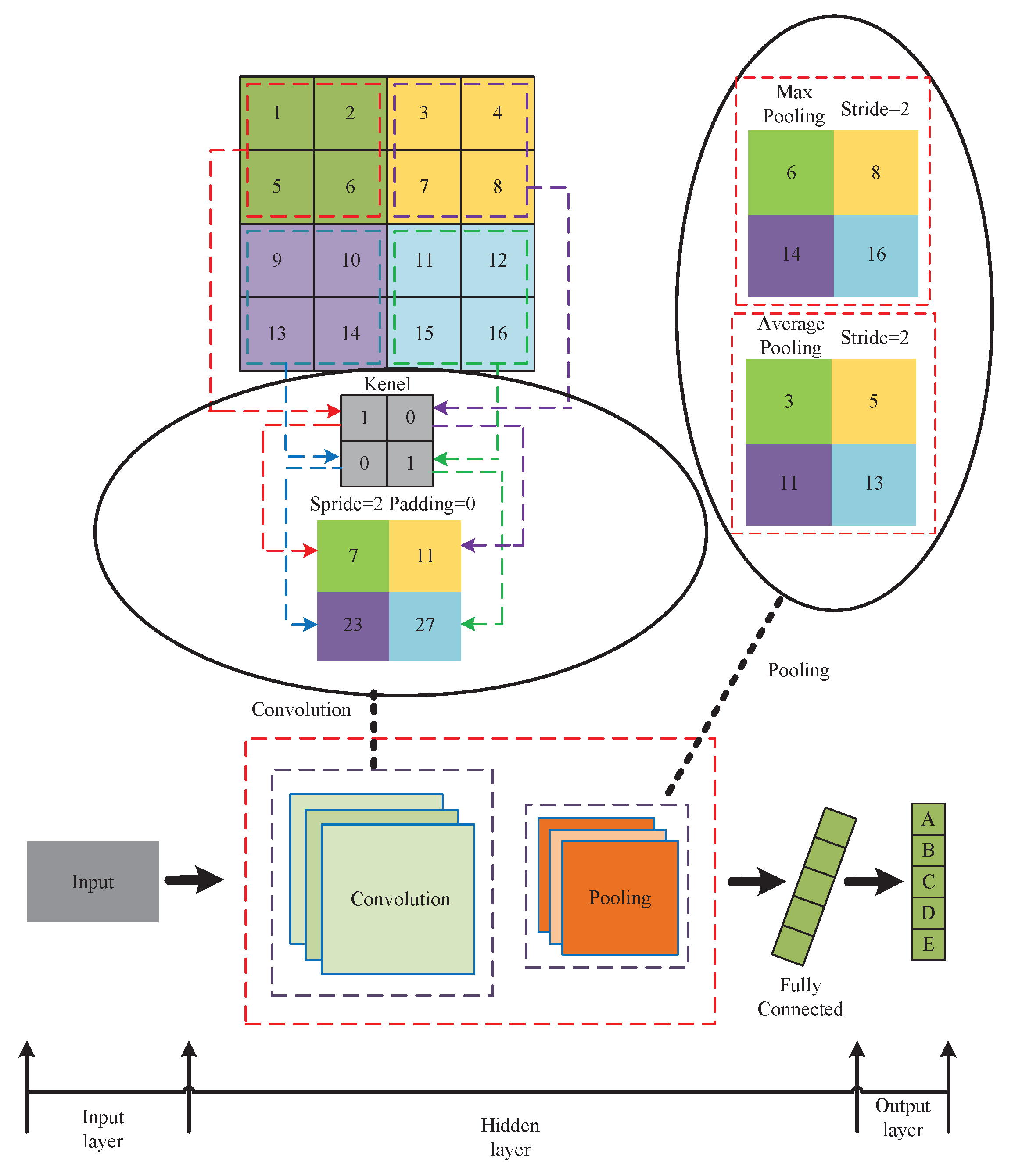
CNNs have made significant breakthroughs in recent years, benefiting from the rapid development of deep learning and artificial neural networks, as well as massive advancements in computing hardware and data storage technologies [31]. CNNs can automatically adjust the weights between neurons and have the advantage of non-linear mapping [32]. CNNs are end-to-end processing mechanisms that usually include a convolutional layer, a pooling layer, and a fully connected layer [33]. Figure 1 depicts the structure of a CNN.

Hidden layers, which include convolutional and pooling layers, are complex neuronal layers with a multilayer non-linear structure. The network can autonomously extract visual characteristics during convolution and pooling without relying on the experience and knowledge of professionals [34]. One of the important components of the convolutional layer is the convolution kernel, which performs feature extraction on the input image. Convolution’s task is to filter the input data and keep the key features to improve the information in the object image. By reducing the number of model parameters and compressing the feature map, the pooling layer aids in the reduction of computing effort.

CNN models benefit from convolution and pooling, with the advantages of translation invariance and weight sharing, and have been widely yet effectively applied to image classification [35]. However, its limitations are relatively obvious. Since the receptive field of CNN is limited by the size of the convolutional kernel, CNNs are limited to modeling relationships between local pixels and cannot represent large distances. The attention technique is used in this research to build global pixel-to-pixel dependencies, which addresses CNNs’ shortcomings.

3.2. Vision Transformer

Vision Transformer (ViT) [14] is the first to apply a pure Transformer architecture to image classification and achieves results comparable to CNN. ViT consists of three main basic modules, patch embedding, encoder, and multilayer perceptron (MLP) classifier. The patch embedding consists of conv2d (16 × 16, stride = 16) and reshape. Multiple vertically stacked Transformer layers form an encoder. The MLP classifier comprises layer normalization and fully connected layers. In the actual execution process, the ViT network first divides the input image (224 × 224 pixels) into 16x16 pixels of non-overlapping patches through patch embedding, reshapes each patch into a one-dimensional token, then concatenates these tokens and a classification token (plus position embedding) is fed to the encoder for encoding, and finally sent to the MLP Classifier for category prediction.

Benefiting from the self-attention mechanism, ViT possesses global modeling ability [36] and achieves satisfactory results on the ImageNet dataset. However, pure Transformer networks like ViT lack the inductive bias of CNNs and thus need to rely on large-scale data to achieve comparable results to CNNs. The increasing abundance of data brings personal privacy breach problems, and data protection is urgent [37]. The emergence of massive data will bring certain risks. According to the priority theorem, relying solely on large-scale data to improve performance is not the best approach; our new idea is to merge CNN and Transformer [38,39].

3.3. Proposed Architecture

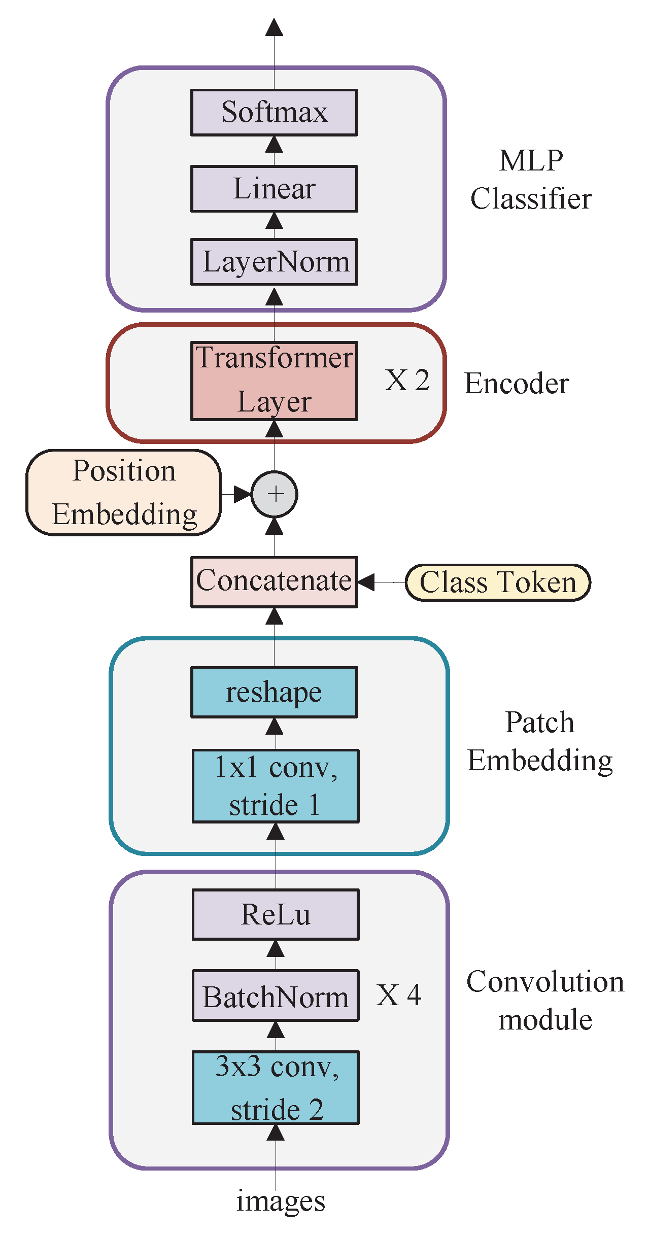
Through the above analysis, we found that CNN and Transformer are complementary. CNN is good at capturing local features while Transformer is skilled at capturing global features. To this end, we construct a hybrid architecture CNN-T that merges CNN and Transformer. CNN-T consists of four parts, convolution module, patch embedding, encoder, and MLP classifier, as shown in Figure 2. The convolution module is employed to extract the image feature map. Patch embedding converts images into sequences of tokens. These tokens concatenate class tokens, plus the positional encoding, and feed into the encoder to extract the high-level semantic information. The MLP performs classification prediction.

The convolution module consists of four standard convolution layers, with a convolution kernel size of 3 and a step size of 2. The convolution kernels number in each layer is 16, 32, 64, and 256, respectively. Each convolution is followed by batch normalization and a rectified linear unit (ReLu) activation operation. Batch Normalization can control the distribution range of the data, effectively avoiding gradient dispersion and explosion.

The patch embedding comprises a convolutional layer (1 × 1, stride = 1) and a reshape operation. The input requirement of the Transformer encoder is 2D (ignoring batch size), so the 3D convolutional feature map (14 × 14 × 128) is reshaped into a 2D shape of 196 × 128.

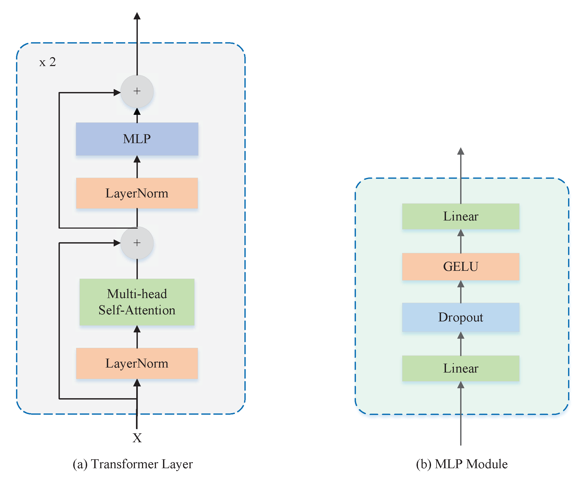
The encoder involves two vertically stacked Transformer layers. As shown in Figure 3a, each Transformer layer consists of two sub-layers. The first sub-layer structure consists of LayerNorm, residual structure, and multi-head self-attention (MHSA). The MHSA number used in this paper is four, and the internal Scaled Dot-Product Attention scoring mechanism has been adopted in MHSA. The second sub-layer structure consists of LayerNorm, Multilayer Perceptron (MLP), and residual structure. The MLP is shown in Figure 3b, which consists of the fully connected layers, the dropout, and the Gaussian Error Linear Units (GELU) activation function superimposed.

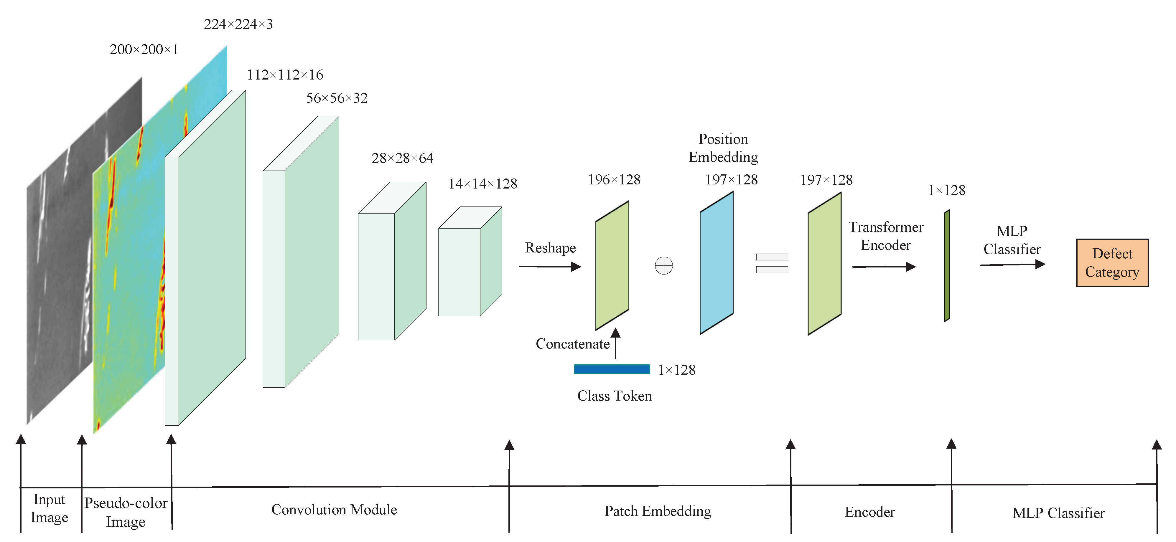
Figure 4 shows the classification system workflow of the CNN-T-based strip steel surface defect. First, the grayscale images in the NEU-CLS dataset are converted to pseudo-color images by the Jet algorithm. Then they are sent to the CNN module for feature extraction to obtain a 14 × 14 × 256 feature map; these feature maps are sent to the patch embedding module for 1 × 1 convolution and reshape operations. Finally, the MLP outputs the classification results.

4. Data Processing

4.1. Experimental Dataset

This paper takes the NEU-CLS dataset collected by Northeastern University as the subject of study. It has been extensively studied in machine vision and experimental results show that datasets have a significant impact on experimental results [40]. The NEU-CLS dataset contains 1800 grayscale images of hot rolled strips of steel surface defects, each with a size of 200 × 200. There are six categories of defects in this dataset, which are cracks (Cr), inclusions (In), patches (Pa), pitted surface (PS), rolled-in scale (RS), and scratches (Sc) [41]. Sample images from the NEU-CLS dataset are shown in Figure 5.

4.2. Pseudo-Color Enhancement

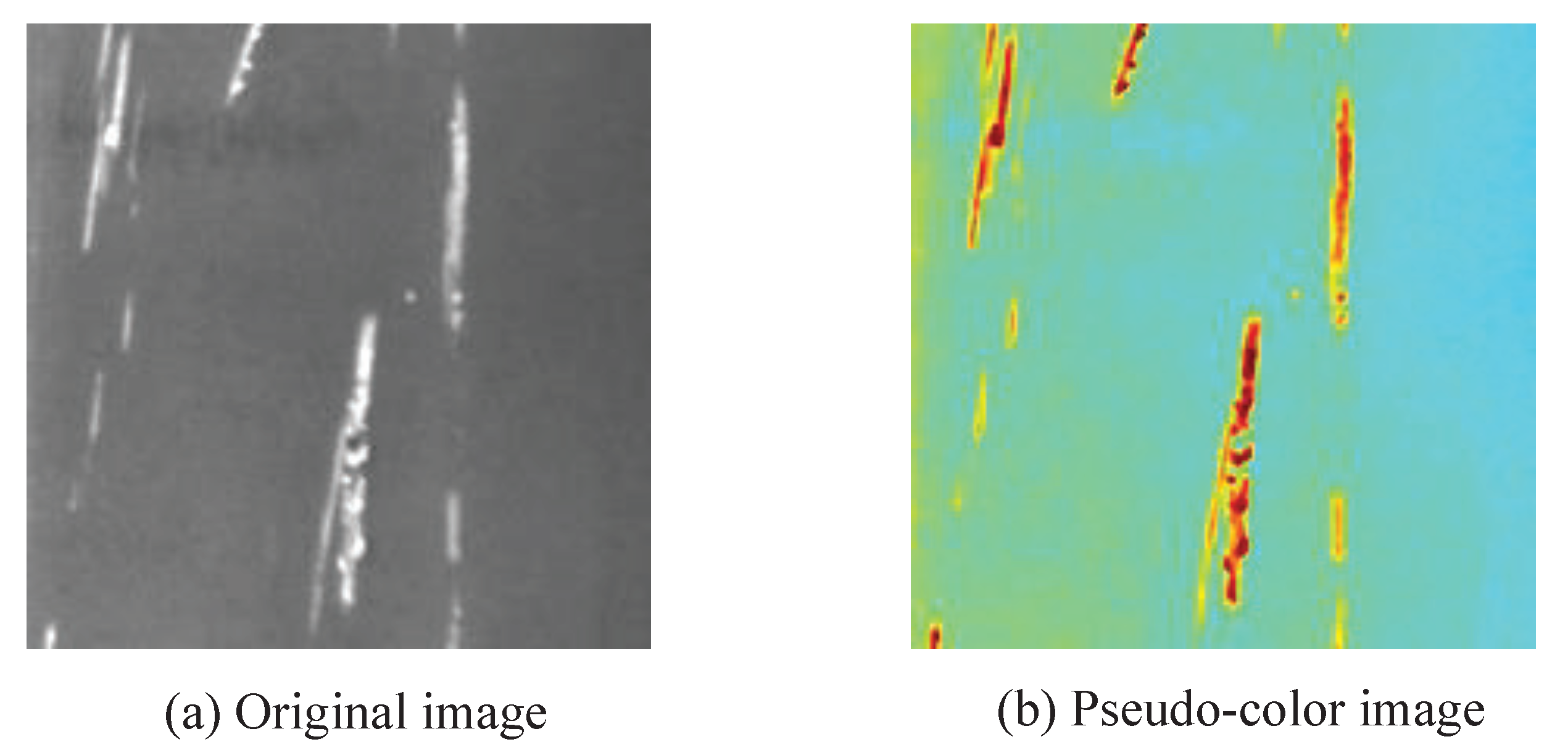
Pseudo-color enhancement is a technology that transforms different grades of grayscale images into various color images according to a linear or nonlinear mapping function. The JET color mapping algorithm is the most commonly used in computer vision, which maps the gray image (0–255) into the pseudo-color image, as shown in Figure 6. The JET mapping algorithm produces pseudo-color images with a high contrast ratio and enhances the information content of the image, which can improve the visual effect of the sample images, effectively highlight the details of the image, and extract features from the sample image [42].

4.3. Data Pre-Processing

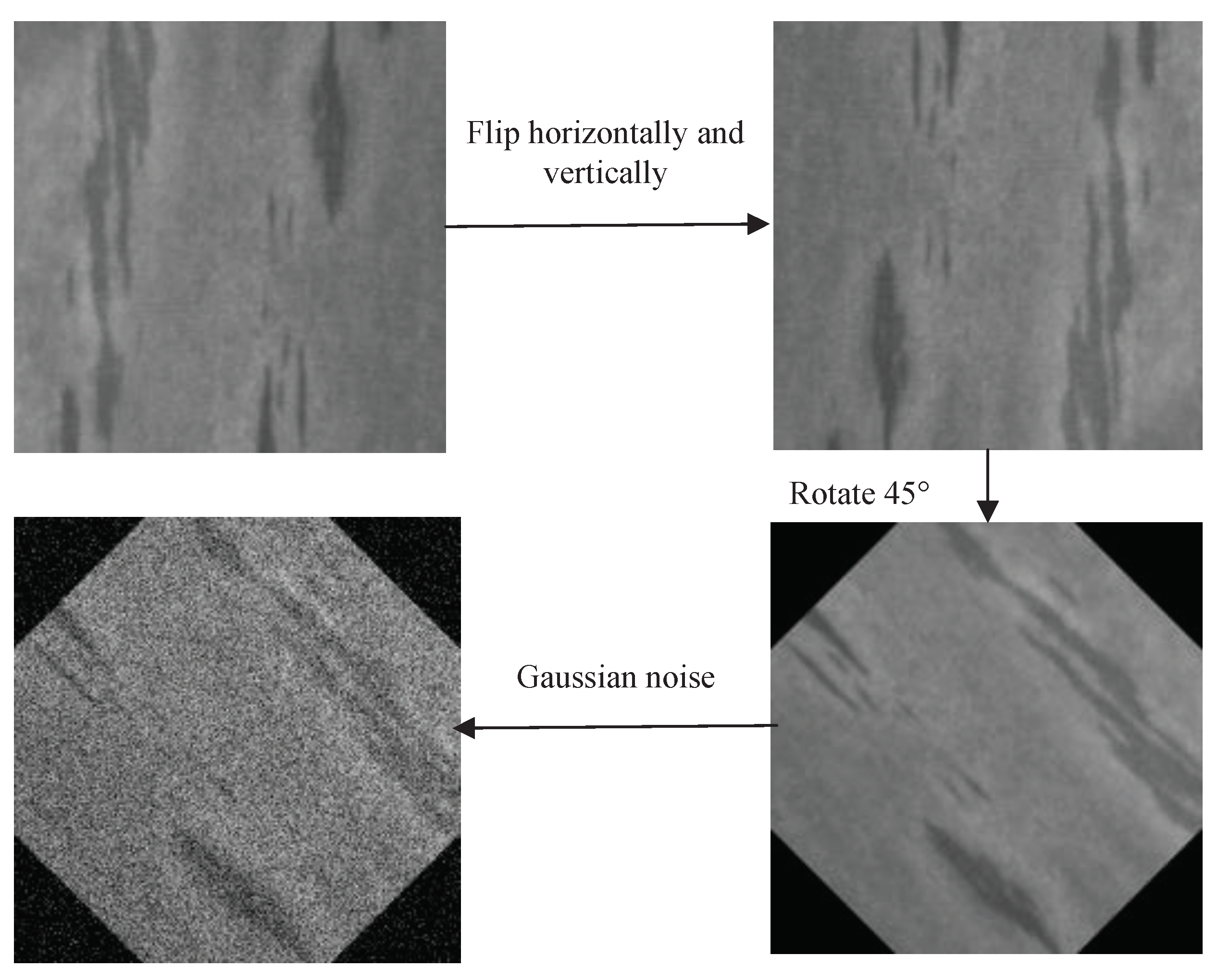
We divide the NEU-CLS dataset into a training set and a test set. Data-driven deep learning models require large samples of training samples [43]. Therefore, we utilize several data augmentation strategies such as Gaussian noise and geometric transformation to expand the training samples to prevent overfitting during model training. Finally, we scale all images to a uniform size of 224 × 224 pixels using bilinear interpolation. Figure 7 introduces the details of the data augmentation.

5. Experiments

5.1. Experimental Setup

We conduct five models in the experiment, GoogLeNet, MobileNet v2, ResNet18, CNN-T, and ViT (ViT consists of six Transformer layers, each of which is the same as the CNN-T’s Transformer layer). We use 70%, 75%, and 80% of the training ratios for training, respectively. The experimental results are random if done only once, which has a large margin of error. The experiment ten times is repeated to reduce the effect of randomness and obtain reliable experimental results. The final result is the average of 10 experiments. The experiment in this paper uses the Pytorch framework, Pycharm development environment, and Python language to implement the proposed approach. The experiments are performed on a server with an Intel(R) Xeon(R) Silver 4210R CPU and a GeForce RTX 2080Ti GPU. The parameter settings have a significant impact on the experimental results. In this paper, the most suitable training strategy and hyperparameters were determined in numerous experiments [44]. The detailed settings of the training are as follows, with Cosine Annealing as the learning rate adjustment strategy, the initial learning rate is 0.002. The loss function uses a cross-entropy function with label smoothing, and the label smoothing factor is set to 0.1. Adam is applied as an optimizer. The weight decay coefficient is 0.001, the batch size is 32, and all models are trained until complete convergence.

5.2. Evaluation Metrics

We evaluate the model’s classification performance through multiple metrics, including accuracy, precision, recall, and F1 score, and use parameters and floating-point operations (FLOPs) to analyze model complexity. The multiclassification problem is treated as multiple dichotomous classification problems, calculate precision, recall, and F1 for all categories, which are given by Equations (1)–(3).

$$\begin{array}{cc}\hfill Precision& \hfill =\frac{TP}{TP+FP}\hfill \end{array}$$

(1)

$$\begin{array}{cc}\hfill Recall& \hfill =\frac{TP}{TP+FN}\hfill \end{array}$$

(2)

$$\begin{array}{cc}\hfill F1& \hfill =\frac{2PR}{P+R}\hfill \end{array}$$

(3)

where $TP$ is True Positive, $TF$ is a True Negative, $FP$ is False Positive, $FN$ is False Negative, P is Precision, and R is Recall. We calculate the total $precision$, $recall$, and $F1$ of all categories, and then average them to obtain the $micro\text{\_}P$, $micro\text{\_}R$, and $micro\text{\_}F1$. The formula is given in (4)–(6).

$$\mathrm{micro}\text{\_}\mathrm{P}=\frac{{\sum }_{i=1}^{n}T{P}_i}{{\sum }_{i=1}^{n}T{P}_i+{\sum }_{i=1}^{n}F{P}_i}$$

(4)

$$\begin{array}{c}\mathrm{micro}\text{\_}\mathrm{R}=\frac{{\sum }_{i=1}^{n}T{P}_i}{{\sum }_{i=1}^{n}T{P}_i+{\sum }_{i=1}^{n}F{N}_i}\end{array}$$

(5)

$$\begin{array}{c}\mathrm{micro}\text{\_}\mathrm{F}1=\frac{2\times \mathrm{micro}\text{\_}\mathrm{P}\times \mathrm{micro}\text{\_}\mathrm{R}}{\mathrm{micro}\text{\_}\mathrm{P}+\mathrm{micro}\text{\_}\mathrm{R}}\end{array}$$

(6)

where n is the category number, which considers various categories’ numbers and is suitable for unbalanced data unbalanced distribution.

5.3. Experimental Results

The accuracy, precision, recall, and F1 of CNN-T and other methods at a training rate of 70% are shown in

Table 1. Accuracy, precision, recall, and F1 of different models when the training ratio is 70%.

Model	Accuracy	Micro_P	Micro_R	Micro_F1
GoogLeNet	96.11%	96.63%	96.11%	96.04%
ResNet18	97.22%	97.46%	97.22%	97.21%
MobileNet v2	98.33%	98.41%	98.33%	98.34%
ViT	95.00%	95.90%	95.00%	94.87%
CNN-T	98.33%	98.44%	98.33%	98.33%

. As shown in Table 1, all the models are above 95% accuracy. Both CNN-T and MobileNet v2 achieved a classification accuracy of 98.33%, but the accuracy of CNN-T was 0.03% higher than that of MobileNet v2. The ViT based on a pure Transformer encoder achieved the worst performance.

Table 2. Accuracy, precision, recall, and F1 of different models when the training ratio is 75%.

Model	Accuracy	Micro_P	Micro_R	Micro_F1
GoogLeNet	97.22%	97.45%	97.22%	97.24%
ResNet18	98.06%	98.26%	98.06%	98.06%
MobileNet v2	98.61%	98.62%	98.61%	98.60%
ViT	96.11%	96.11%	96.11%	96.10%
CNN-T	98.89%	98.96%	98.89%	98.89%

gives the accuracy, precision, recall, and F1 of different models at a training rate of 75%. As can be seen from Table 2, all models achieved a better than training ratio of 70%. This suggests that the performance of supervised learning models is mainly dependent on the number of training samples. When the training ratio was 75%, all models except ViT achieved F1 above 98%. Our method achieved the best performance, followed by MobileNet v2.

The accuracy, precision, recall, and F1 of different models at a training rate of 80% are shown in

Table 3. Accuracy, precision, recall, and F1 of different models when the training ratio is 80%.

Model	Accuracy	Micro_P	Micro_R	Micro_F1
GoogLeNet	98.06%	98.18%	98.06%	98.03%
ResNet18	98.33%	98.35%	98.33%	98.34%
MobileNet v2	98.89%	98.93%	98.89%	98.89%
ViT	96.94%	97.18%	96.94%	96.91%
CNN-T	99.17%	99.21%	99.17%	99.17%

. As can be seen from Table 3, CNN-T achieved the top results for all metrics, accuracy, precision, recall, and F1 of 99.17%, 99.21%, 99.17%, and 99.17%, respectively. MobileNet v2 achieved the second-place result, and the accuracy was 0.83%, 0.56%, and 1.95% higher than GoogLeNet, ResNet, and ViT, respectively. At 70%, 75%, and 80% training ratios, our method achieved optimal performance compared to GoogLeNet, ResNet18, MobileNet v2, and ViT. This demonstrates the effectiveness and superiority of CNN-T for strip steel’s surface defect classification.

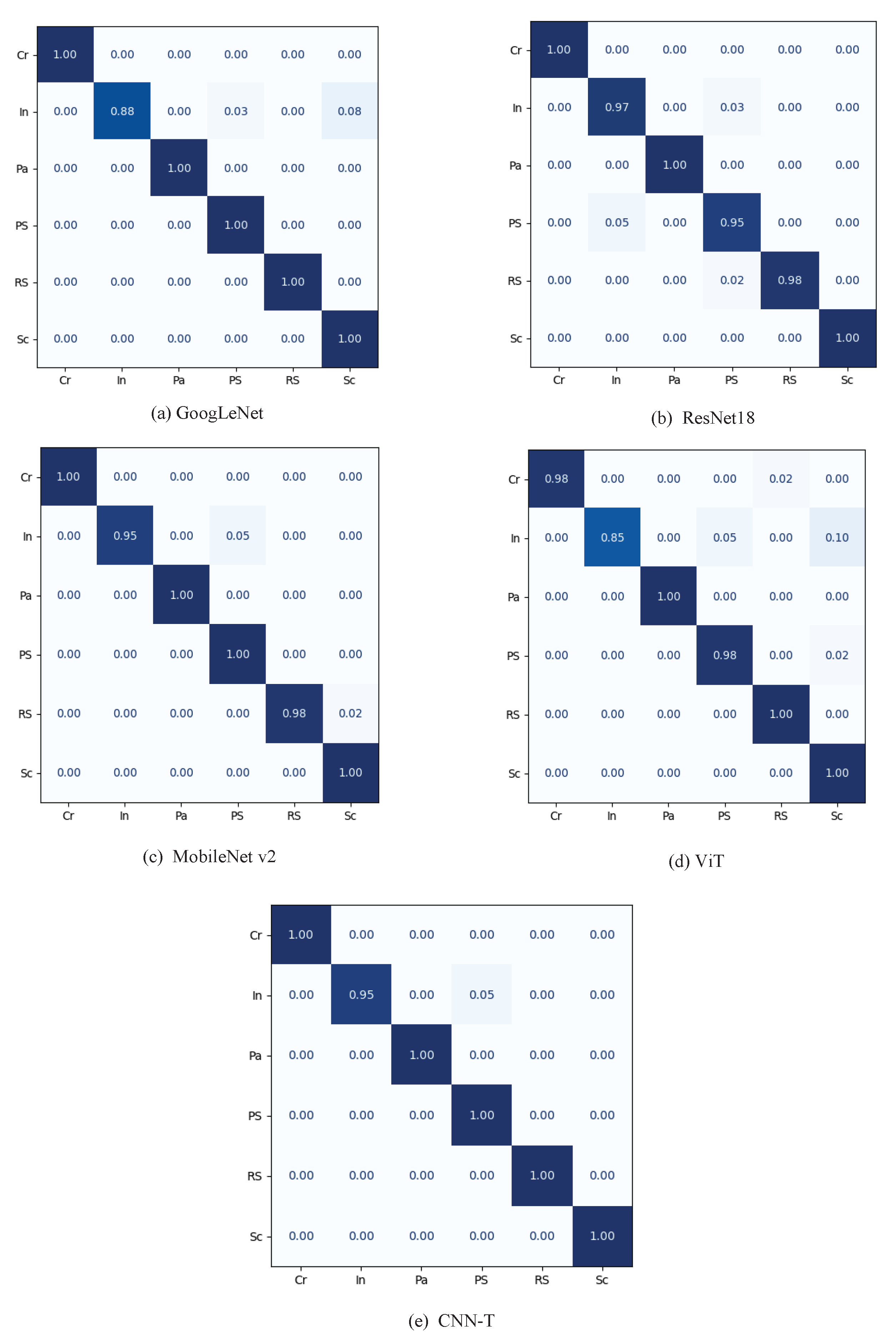
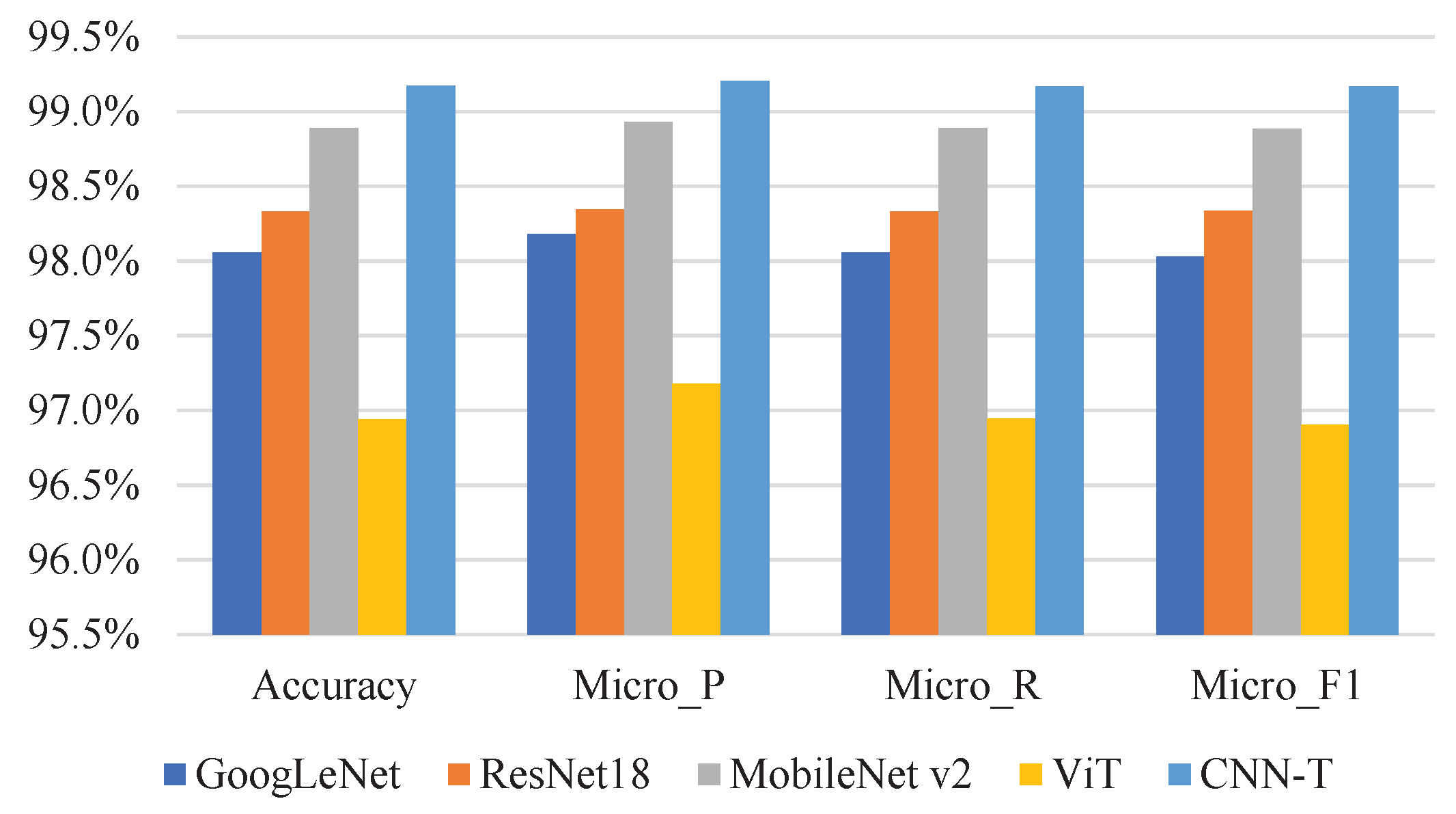
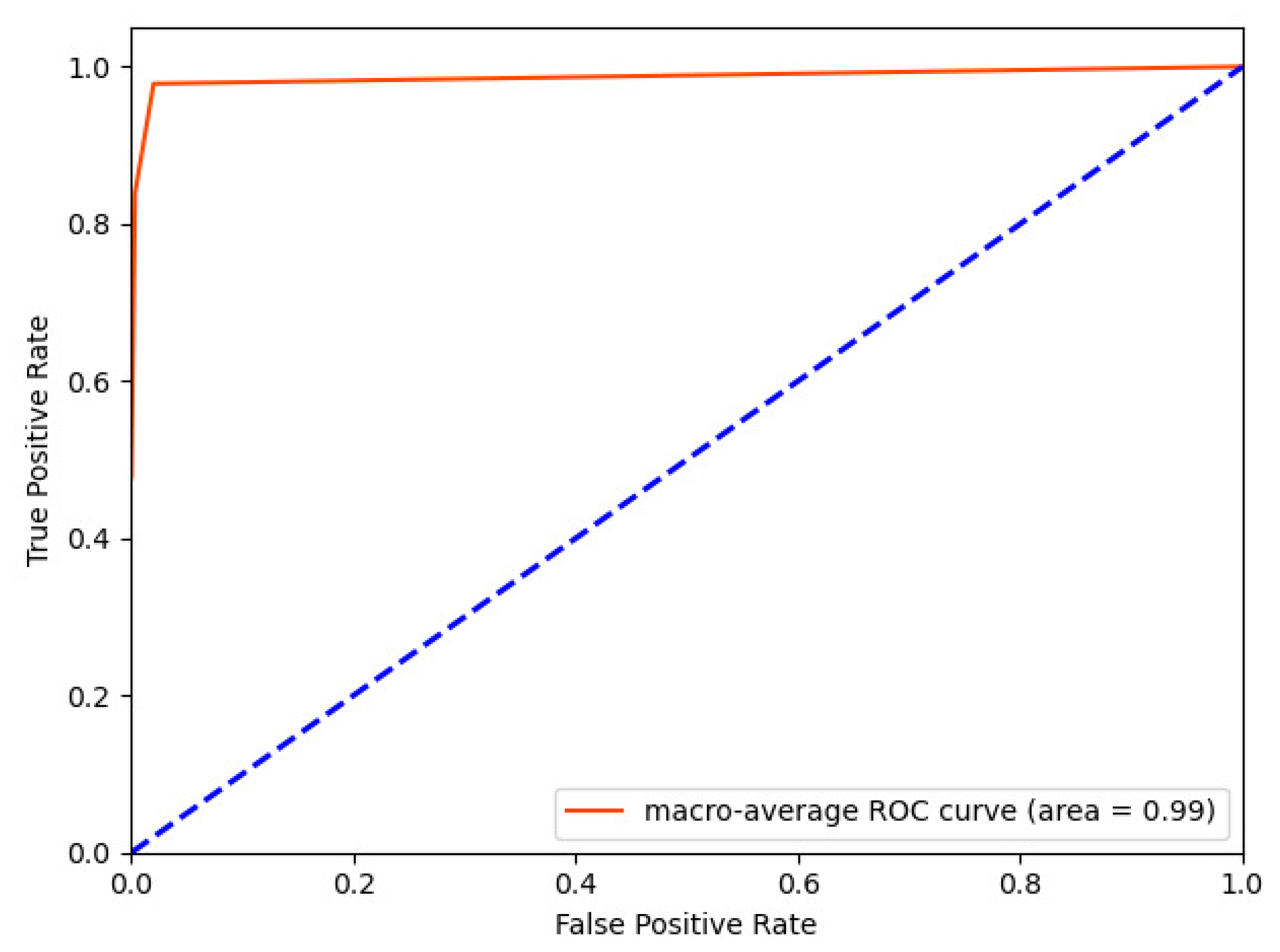
To further illustrate the effectiveness of the proposed method, we present the confusion matrices of all models with a training ratio of 80%, as shown in Figure 8. To more intuitively see the classification results of the above model (training ratio of 80%), we display them as bar graphs, as shown in Figure 9. We also give the ROC curve of the proposed method on the test set with a training ratio of 80%, as shown in Figure 10.

The performance of a classification model depends not only on accuracy but also on the complexity of the model. We analyzed all model complexity in our experiments through two measures of model parameters and FLOPs. As shown in

Table 4. Comparison of models parameters and FLOPs.

Model	Params(M)	FLOPs(G)
GoogLeNet	11.99	1.51
ResNet18	11.18	1.82
MobileNet v2	2.23	0.32
ViT	0.89	0.17
CNN-T	0.48	0.12

, CNN-T has the lowest parameters compared to other models, only 0.48 M. The FLOPs of the proposed architecture is only about 8% of that of GoogLeNet, and also much lower than MibileNet v2, ResNet, and ViT.

6. Discussions

In this paper, we demonstrate the importance of global discriminative features for accurately classifying strip surface defects. We utilize an attention-based Transformer encoder to globally model local features extracted from CNN, which can obtain contextual semantic information from images. Experimental results show that our proposed method is feasible and effective. Specifically, it outperforms pure Transformer networks and CNNs (e.g., GoogLeNet, MobileNet v2, ResNet18) on the NEU-CLS dataset (training ratio is 80%) with a 0.28–2.23% improvement in classification accuracy, with fewer parameters (0.45 M) and FLOPs (0.12 G).

The CNN is known to be effective in capturing local patterns, while the Transformer encoder is good at understanding context, but it is heavy (e.g., it has a lot of parameters). Thus, the purpose of the combination of CNN and Transformer encoder is that CNN converts the input image to a compact representation (which prevents the entire model from being too large), and the Transformer encoder finds global, higher-level patterns from the compact representation. Although the proposed method is effective, it is trained based on supervised learning, which requires a certain scale of labeled data. Therefore, semi-supervised or unsupervised training would greatly alleviate the reliance on labeled data by pre-training or further improving the proposed method on large-scale datasets.

7. Conclusions

CNNs have dominated the classification task for surface defects in strip steel. However, CNNs with local receptive fields cannot extract global semantic information from images, which hinders the accurate classification of surface defects of strip steel. This paper proposes a hybrid architecture based on CNN and Transformer to overcome this problem, which inherits the excellent properties of both CNN and Transformer, such as inductive bias and global representation ability. Specifically, the CNN converts the input image to a compact representation (which prevents the entire model from being too large), and the Transformer encoder finds global, higher-level patterns from the compact representation. In addition, we use data augmentation strategies such as geometric transformation, color change, and Gaussian Gaussian to enrich the number and diversity of training samples. Extensive experiments show that CNN-T outperforms pure Transformers and some CNNs (e.g., GoogLeNet, MobileNet v2, and ResNet18) on the NEU-CLS dataset, with fewer parameters and FLOPs.

References

- Aldunin, A. Development of method for calculation of structure parameters of hot-rolled steel strip for sheet stamping. J. Chem. Technol. Metall. 2017, 52, 737–740. [Google Scholar]
- Xu, Z.W.; Liu, X.M.; Zhang, K. Mechanical properties prediction for hot rolled alloy steel using convolutional neural network. IEEE Access 2019, 7, 47068–47078. [Google Scholar] [CrossRef]
- Ren, Q.; Geng, J.; Li, J. Slighter Faster R-CNN for real-time detection of steel strip surface defects. In Proceedings of the IEEE 2018 Chinese Automation Congress (CAC), Xi’an, China, 30 November–2 December 2018; pp. 2173–2178. [Google Scholar]
- He, D.; Xu, K.; Zhou, P. Defect detection of hot rolled steels with a new object detection framework called classification priority network. Comput. Ind. Eng. 2019, 128, 290–297. [Google Scholar] [CrossRef]
- Jeon, M.; Jeong, Y.S. Compact and accurate scene text detector. Appl. Sci. 2020, 10, 2096. [Google Scholar] [CrossRef] [Green Version]
- Vu, T.; Van Nguyen, C.; Pham, T.X.; Luu, T.M.; Yoo, C.D. Fast and efficient image quality enhancement via desubpixel convolutional neural networks. In Proceedings of the European Conference on Computer Vision (ECCV) Workshops, Munich, Germany, 8–14 September 2018. [Google Scholar]
- He, K.; Zhang, X.; Ren, S.; Sun, J. Deep residual learning for image recognition. In Proceedings of the IEEE Conference on Computer Vision and Pattern Recognition, Las Vegas, NV, USA, 27–30 June 2016; pp. 770–778. [Google Scholar]
- Iandola, F.N.; Han, S.; Moskewicz, M.W.; Ashraf, K.; Dally, W.J.; Keutzer, K. SqueezeNet: AlexNet-level accuracy with 50x fewer parameters and <0.5 MB model size. arXiv 2016, arXiv:1602.07360. [Google Scholar]
- Zhang, X.; Zhou, X.; Lin, M.; Sun, J. Shufflenet: An extremely efficient convolutional neural network for mobile devices. In Proceedings of the IEEE conference on computer vision and pattern recognition, Salt Lake City, UT, USA, 18–23 June 2018; pp. 6848–6856. [Google Scholar]
- Howard, A.G.; Zhu, M.; Chen, B.; Kalenichenko, D.; Wang, W.; Weyand, T.; Andreetto, M.; Adam, H. Mobilenets: Efficient convolutional neural networks for mobile vision applications. arXiv 2017, arXiv:1704.04861. [Google Scholar]
- Wang, Z.; Lu, W.; He, Y.; Xiong, N.; Wei, J. Re-CNN: A robust convolutional neural networks for image recognition. In Proceedings of the International Conference on Neural Information Processing, Siem Reap, Cambodia, 13–16 December 2018; Springer: Cham, Switzerland, 2018; pp. 385–393. [Google Scholar]
- Vaswani, A.; Shazeer, N.; Parmar, N.; Uszkoreit, J.; Jones, L.; Gomez, A.N.; Kaiser; Polosukhin, I. Attention is all you need. Adv. Neural Inf. Process. Syst. 2017, 30. [Google Scholar]
- Liu, Y.; Zhang, Y.; Wang, Y.; Hou, F.; Yuan, J.; Tian, J.; Zhang, Y.; Shi, Z.; Fan, J.; He, Z. A Survey of Visual Transformers. arXiv 2021, arXiv:2111.06091. [Google Scholar]
- Dosovitskiy, A.; Beyer, L.; Kolesnikov, A.; Weissenborn, D.; Zhai, X.; Unterthiner, T.; Dehghani, M.; Minderer, M.; Heigold, G.; Gelly, S.; et al. An image is worth 16x16 words: Transformers for image recognition at scale. arXiv 2020, arXiv:2010.11929. [Google Scholar]
- Vannocci, M.; Ritacco, A.; Castellano, A.; Galli, F.; Vannucci, M.; Iannino, V.; Colla, V. Flatness defect detection and classification in hot rolled steel strips using convolutional neural networks. In Proceedings of the International Work-Conference on Artificial Neural Networks, Gran Canaria, Spain, 12–14 June 2019; Springer: Cham, Switzerland, 2019; pp. 220–234. [Google Scholar]
- Gao, Y.; Xiang, X.; Xiong, N.; Huang, B.; Lee, H.J.; Alrifai, R.; Jiang, X.; Fang, Z. Human action monitoring for healthcare based on deep learning. IEEE Access 2018, 6, 52277–52285. [Google Scholar] [CrossRef]
- Wu, C.; Ju, B.; Wu, Y.; Lin, X.; Xiong, N.; Xu, G.; Li, H.; Liang, X. UAV autonomous target search based on deep reinforcement learning in complex disaster scene. IEEE Access 2019, 7, 117227–117245. [Google Scholar] [CrossRef]
- Luo, Q.; He, Y. A cost-effective and automatic surface defect inspection system for hot-rolled flat steel. Robot. Comput.-Integr. Manuf. 2016, 38, 16–30. [Google Scholar] [CrossRef]
- Ashour, M.W.; Khalid, F.; Abdul Halin, A.; Abdullah, L.N.; Darwish, S.H. Surface defects classification of hot-rolled steel strips using multi-directional shearlet features. Arab. J. Sci. Eng. 2019, 44, 2925–2932. [Google Scholar] [CrossRef]
- Gong, R.; Wu, C.; Chu, M. Steel surface defect classification using multiple hyper-spheres support vector machine with additional information. Chemom. Intell. Lab. Syst. 2018, 172, 109–117. [Google Scholar] [CrossRef]
- Liu, K.; Li, A.; Wen, X.; Chen, H.; Yang, P. Steel surface defect detection using GAN and one-class classifier. In Proceedings of the IEEE 2019 25th International Conference on Automation and Computing (ICAC), Lancaster, UK, 5–7 September 2019; pp. 1–6. [Google Scholar]
- Goodfellow, I.; Pouget-Abadie, J.; Mirza, M.; Xu, B.; Warde-Farley, D.; Ozair, S.; Courville, A.; Bengio, Y. Generative adversarial nets. Adv. Neural Inf. Process. Syst. 2014, 27. [Google Scholar]
- Liu, Y.; Geng, J.; Su, Z.; Zhang, W.; Li, J. Real-time classification of steel strip surface defects based on deep CNNs. In Proceedings of 2018 Chinese Intelligent Systems Conference; Springer: Singapore, 2019; pp. 257–266. [Google Scholar]
- Fu, G.; Sun, P.; Zhu, W.; Yang, J.; Cao, Y.; Yang, M.Y.; Cao, Y. A deep-learning-based approach for fast and robust steel surface defects classification. Opt. Lasers Eng. 2019, 121, 397–405. [Google Scholar] [CrossRef]
- Boudiaf, A.; Benlahmidi, S.; Harrar, K.; Zaghdoudi, R. Classification of Surface Defects on Steel Strip Images using Convolution Neural Network and Support Vector Machine. J. Fail. Anal. Prev. 2022, 22, 531–541. [Google Scholar] [CrossRef]
- Szegedy, C.; Liu, W.; Jia, Y.; Sermanet, P.; Reed, S.; Anguelov, D.; Erhan, D.; Vanhoucke, V.; Rabinovich, A. Going deeper with convolutions. In Proceedings of the IEEE Conference on Computer Vision and Pattern Recognition, Boston, MA, USA, 7–12 June 2015; pp. 1–9. [Google Scholar]
- Krizhevsky, A.; Sutskever, I.; Hinton, G.E. Imagenet classification with deep convolutional neural networks. Adv. Neural Inf. Process. Syst. 2012, 25, 1097–1105. [Google Scholar] [CrossRef]
- He, C.; Chen, S.; Huang, S.; Zhang, J.; Song, X. Using convolutional neural network with BERT for intent determination. In Proceedings of the IEEE 2019 International Conference on Asian Language Processing (IALP), Shanghai, China, 5–17 November 2019; pp. 65–70. [Google Scholar]
- Devlin, J.; Chang, M.W.; Lee, K.; Toutanova, K. Bert: Pre-training of deep bidirectional transformers for language understanding. arXiv 2018, arXiv:1810.04805. [Google Scholar]
- Wu, H.; Xiao, B.; Codella, N.; Liu, M.; Dai, X.; Yuan, L.; Zhang, L. Cvt: Introducing convolutions to vision transformers. In Proceedings of the IEEE/CVF International Conference on Computer Vision, Montreal, BC, Canada, 11–17 October 2021; pp. 22–31. [Google Scholar]
- Huang, S.; Liu, A.; Zhang, S.; Wang, T.; Xiong, N.N. BD-VTE: A novel baseline data based verifiable trust evaluation scheme for smart network systems. IEEE Trans. Netw. Sci. Eng. 2020, 8, 2087–2105. [Google Scholar] [CrossRef]
- Gao, K.; Han, F.; Dong, P.; Xiong, N.; Du, R. Connected vehicle as a mobile sensor for real time queue length at signalized intersections. Sensors 2019, 19, 2059. [Google Scholar] [CrossRef] [PubMed] [Green Version]
- Tang, H.; Wang, Y.; Yang, X. Evaluation of Visualization Methods’ Effect on Convolutional Neural Networks Research. In Proceedings of the 2018 International Conference on Algorithms, Computing and Artificial Intelligence, Sanya, China, 21–23 December 2018; pp. 1–5. [Google Scholar]
- Cheng, H.; Xie, Z.; Shi, Y.; Xiong, N. Multi-step data prediction in wireless sensor networks based on one-dimensional CNN and bidirectional LSTM. IEEE Access 2019, 7, 117883–117896. [Google Scholar] [CrossRef]
- Xiong, N.; He, J.S.; Park, J.H.; Cooley, D. A Neutral Network Based Vehicle Classification System for Pervasive Smart Road Security. J. Univers. Comput. Sci. 2009, 15, 1119. [Google Scholar]
- Cordonnier, J.B.; Loukas, A.; Jaggi, M. On the relationship between self-attention and convolutional layers. arXiv 2019, arXiv:1911.03584. [Google Scholar]
- Yang, P.; Xiong, N.; Ren, J. Data security and privacy protection for cloud storage: A survey. IEEE Access 2020, 8, 131723–131740. [Google Scholar] [CrossRef]
- Zhang, X.; Jin, Y.; Kwak, K.S. Adaptive GTS allocation scheme with applications for real-time Wireless Body Area Sensor Networks. KSII Trans. Internet Inf. Syst. (TIIS) 2015, 9, 1733–1751. [Google Scholar]
- Wang, Y.; Li, X.; Gao, Y.; Wang, L.; Gao, L. A new Feature-Fusion method based on training dataset prototype for surface defect recognition. Adv. Eng. Inform. 2021, 50, 101392. [Google Scholar] [CrossRef]
- Wu, M.; Tan, L.; Xiong, N. A structure fidelity approach for big data collection in wireless sensor networks. Sensors 2014, 15, 248–273. [Google Scholar] [CrossRef] [Green Version]
- Li, K.; Wang, X.; Ji, L. Application of multi-scale feature fusion and deep learning in detection of steel strip surface defect. In Proceedings of the IEEE 2019 International Conference on Artificial Intelligence and Advanced Manufacturing (AIAM), Dublin, Ireland, 17–19 October 2019; pp. 656–661. [Google Scholar]
- Potashnikov, A.; Vlasuyk, I.; Ivanchev, V.; Balobanov, A. The method of representing grayscale images in pseudo color using equal-contrast color space. In Proceedings of the IEEE 2020 Systems of Signals Generating and Processing in the Field of on Board Communications, Moscow, Russia, 19–20 March 2020; pp. 1–6. [Google Scholar]
- Wu, P.; Wu, G.; Wu, X.; Yi, X.; Xiong, N. Birds Classification Based on Deep Transfer Learning. In Proceedings of the International Conference on Smart Computing and Communication, Paris, France, 29–31 December 2020; Springer: Cham, Switzerland, 2020; pp. 173–183. [Google Scholar]
- Li, H.; Liu, J.; Wu, K.; Yang, Z.; Liu, R.W.; Xiong, N. Spatio-temporal vessel trajectory clustering based on data mapping and density. IEEE Access 2018, 6, 58939–58954. [Google Scholar] [CrossRef]
Figure 1.
Structure of the CNN.
Figure 2.
CNN-T architecture.
Figure 3.
Transformer layer and MLP module.
Figure 4.
CNN-T workflow. The numbers on the label respectively indicate the height, width, and channels of the feature map.
Figure 5.
Sample images in the NEU-CLS dataset.
Figure 6.
Pseudo-color enhancement effect. (a) original image, (b) pseudo-color image.
Figure 7.
Data preprocessing. Flip, flip the image horizontally and vertically. Rotation, rotate the picture 45 degrees separately. Random crop, randomly crop different parts of the picture. Add noise, add Gaussian noise to the picture.
Figure 8.
Confusion matrix of models. (a) GoogLeNet, (b) ResNet18, (c) MobileNet v2, (d) ViT, (e) CNN-T.
Figure 9.
Accuracy, precision, recall, and F1 of CNN-T and reference models when the training ratio is 80%.
Figure 10.
ROC curve of the proposed method on the test set with a training ratio is 80%.